Spin-thermopower in interacting quantum dots

Abstract

Using analytical arguments and the numerical renormalization group method we investigate the spin-thermopower of a quantum dot in a magnetic field. In the particle-hole symmetric situation the temperature difference applied across the dot drives a pure spin current without accompanying charge current. For temperatures and fields at or above the Kondo temperature, but of the same order of magnitude, the spin-Seebeck coefficient is large, of the order of $k_{B}/|e|$. Via a mapping, we relate the spin-Seebeck coefficient to the charge-Seebeck coefficient of a negative-$U$ quantum dot where the corresponding result was recently reported by Andergassen et al. in Phys. Rev. B 84, 241107 (2011). For several regimes we provide simplified analytical expressions. In the Kondo regime, the dependence of the spin-Seebeck coefficient on the temperature and the magnetic field is explained in terms of the shift of the Kondo resonance due to the field and its broadening with the temperature and the field. We also consider the influence of breaking the particle-hole symmetry and show that a pure spin current can still be realized provided a suitable electric voltage is applied across the dot. Then, except for large asymmetries, the behavior of the spin-Seebeck coefficient remains similar to that found in the particle-hole symmetric point.

I Introduction

Thermoelectricity is the occurrence of electric voltages in the presence of temperature differences or vice-versa. Devices based on thermoelectric phenomena can be used for several applications including power generation, refrigeration, and temperature measurement.Mahan et al. (1997) Thermoelectric phenomena are also of fundamental scientific interest as they reveal information about a system which is unavailable in standard charge transport measurements.Segal (2005) Recent reinvigoration in this field is due to a large thermoelectric response found in some strongly correlated materials, e.g. sodium cobaltate,Terasaki et al. (1997) as well as due to the investigation of thermopower in nanoscale junctions such as quantum point contacts, silicon nanowires, carbon nanotubes, and molecular junctions.Dubi and Di Ventra (2011); Rejec et al. (2002) Recently, thermopower of Kondo correlated quantum dots has been measuredScheibner et al. (2005) and theoretically analyzed.Costi and Zlatić (2010); Andergassen et al. (2011)

Importantly, the thermoelectric effects turned to be usefulUchida et al. (2008) also for spintronicsŽutić et al. (2004). Spintronic devices exploiting the spin degree of freedom of an electron, such as the prototypical Datta-Das spin field-effect transistor,Datta and Das (1990) promise many advantages over the conventional charge-based electronic devices, most notably lower power consumption and heating.Wolf et al. (2001) Recently, the spin-Hall effect was utilized to realize the spin transistor idea experimentally.Wunderlich et al. (2010) Generating spin currents plays a fundamental role in driving spintronic devices. Several methods of generating spin currents have been put forward such as electrical based on the tunneling from ferromagnetic contacts and optical based on excitation of carriers in semiconductors with circularly polarized light.Žutić et al. (2004) Another possibility is thermoelectrical injection. In a recent breakthrough, the spin-Seebeck effect, where the spin current is driven by a temperature difference across the sample, has been observed in a metallic ferromagnet and suggested as a spin current source.Uchida et al. (2008)

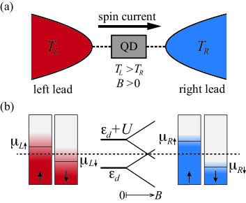
Figure 1: (a) Quantum dot attached to paramagnetic leads held at different temperatures. (b) Energy levels in the leads and in the quantum dot (at the particle-hole symmetric point, as a function of the magnetic field).

Some of the above mentioned methods have an undesirable property that the generated spin current is accompanied by an electrical current, which leads to dissipation and heat. In this paper we consider a device, which uses the spin-Seebeck effect to generate a pure spin current. It consists of a quantum dot in a magnetic field attached to paramagnetic leads, as shown in Fig. 1(a). The leads are held at different temperatures. In the particle-hole symmetric situation, this setup generates a pure spin current across the quantum dot. Away from the particle-hole symmetric point, a pure spin current can be generated provided a suitable electrical voltage is applied. By tuning the temperature and the magnetic field, large values of the spin-Seebeck coefficient of the order of $k_{B}/|e|$ can be reached. For the particle-hole symmetric case this was first recognized in a related problem of the charge thermopower in a negative-$U$ quantum dot by Andergassen et al. in Ref. [Andergassen et al., 2011].

The outline of the paper is as follows. First, in Secs. II and III, we present the model and introduce the notion of spin-thermopower and define the spin-Seebeck coefficient. In Sec. IV, we present exact results for a device containing a noninteracting quantum dot. Then, in Sec. V, we describe the details of the numerical renormalization group (NRG) calculation and, in Sec. VI, we present the NRG results for a device with an interacting quantum dot. We also derive analytical expressions for the spin-Seebeck coefficient in several asymptotic regimes and find the boundaries between those regimes. Finally, in Sec. VII, we give conclusions and examine whether our results can be easily observed experimentally. In Appendix A we present an intuitive explanation why a pure spin current is generated in the particle-hole symmetric point.

The spin-Seebeck coefficient was calculated for a single-molecule-magnet attached to metallic electrodesWang et al. (2010) and for a quantum dot in contact with ferromagnetic electrodes,Dubi and Di Ventra (2009) both within the sequential tunneling approximation. The later system was also analyzed using the equation of motion techniqueŚwirkowicz et al. (2009) as well as the Hartree-Fock approximation.Ying and Jin (2010) All these methods fail to describe correctly the effects of Kondo correlations occurring at low temperatures and magnetic fields in such systems. Thermospin effects in quasi-one dimensional quantum wires in the presence of a magnetic field and Rashba spin-orbit interaction were also studied theoretically.Lu et al. (2010)

II Model

Our starting point is the standard Anderson impurity HamiltonianHewson (1993)

$$H = \sum_{\sigma}\left(\epsilon_{d}+\sigma\frac{B}{2}\right)n_{d\sigma}+Un_{d\uparrow}n_{d\downarrow}+$$ (1)

$$+\sum_{k\alpha\sigma}\varepsilon_{k\alpha}c_{k\alpha\sigma}^{\dagger}c_{k\alpha\sigma}+\sum_{k\alpha\sigma}V_{k\alpha}c_{k\alpha\sigma}^{\dagger}d_{\sigma}+\mathrm{h.c.}$$

Here we assume that only the highest occupied energy level $\epsilon_{d}$ in the dot is relevant for the transport properties. Due to the electron’s spin $\sigma=\pm 1$, in external magnetic field this level is split by the Zeeman energy $g\mu_{B}B$. Rather than by an external magnetic field, the dot level could also be split by a local exchange field due to an attached ferromagnetic electrode.Martinek et al. (2005) To keep the notation short, in Eq. (1) we express the magnetic field in energy units, i.e., $g\mu_{B}=1$. $U$ is the Coulomb charging energy of the dot, while $\Gamma=\sum_{\alpha}\Gamma_{\alpha}$ is the total hybridization, where $-i\Gamma_{\alpha}=\sum_{k}\left|V_{k\alpha}\right|^{2}/\left(\omega-\epsilon_{k\alpha}+i\delta\right)$ is the hybridization function of the dot level with the states in the left ($\alpha=L$) and the right ($\alpha=R$) lead, which we assume to be energy independent, as appropriate for wide bands in leads with constant densities of states. Furthermore, we will mostly consider the system at the particle-hole symmetric point (in experiments, the deviation from particle-hole symmetry is easily controlled by the gate voltage) where the dot level is at $\epsilon_{d}=\mu-\frac{U}{2}$ in equilibrium. In what follows we set the equilibrium chemical potential $\mu$ to zero. In such a regime the spin of the quantum dot is quenched at temperatures (again we use the energy units, $k_{B}=1$) and magnetic fields low compared to the Kondo temperatureHorvatic and Zlatic (1985)

$$T_{K}=\sqrt{\frac{U\Gamma}{2}}e^{-\frac{\pi U}{8\Gamma}+\frac{\pi\Gamma}{2U}}.$$ (2)

To describe the system away from the particle-hole symmetric point we introduce the asymmetry parameter $\delta=\epsilon_{d}+\frac{U}{2}$.

III Spin-Seebeck coefficient

In a non-equilibrium situation the distribution of electrons with spin $\sigma$ in the lead $\alpha$ is described by the Fermi-Dirac distribution function $f_{\alpha\sigma}\left(\omega\right)=1/\left[e^{\left(\omega-\mu_{\alpha\sigma}\right)/T_{\alpha}}+1\right]$ with $\mu_{\alpha\sigma}$ and $T_{\alpha}$ being the spin dependent chemical potentials and the temperature in the lead $\alpha$, respectively [Fig. 1(b)]. The electrical current of electrons with spin $\sigma$ is

$$I_{\sigma}=\frac{e}{h}\int\mathrm{d}\omega\left[f_{L\sigma}\left(\omega\right)-f_{R\sigma}\left(\omega\right)\right]{\cal T}_{\sigma}\left(\omega\right),$$ (3)

where $e$ is the electron charge, $h$ is the Planck constant, and ${\cal T}_{\sigma}\left(\omega\right)=\pi\frac{2\Gamma_{L}\Gamma_{R}}{\Gamma_{L}+\Gamma_{R}}A_{\sigma}\left(\omega\right)$ is the transmission function of electrons with spin $\sigma$.Meir and Wingreen (1992) It is calculated from the impurity spectral function $A_{\sigma}\left(\omega\right)=-\frac{1}{\pi}\mathrm{Im}G_{\sigma}\left(\omega\right)$ where

$$G_{\sigma}\left(\omega\right)=\frac{1}{\omega-\epsilon_{d}-\sigma\frac{B}{2}+i\Gamma-\Sigma_{\sigma}\left(\omega\right)}$$

is the retarded impurity Green’s function and the interaction self-energy $\Sigma_{\sigma}\left(\omega\right)$ accounts for the many-body effects. Introducing the average chemical potential in each of the leads,

$$\mu_{\alpha}=\frac{1}{2}\left(\mu_{\alpha\uparrow}+\mu_{\alpha\downarrow}\right),$$

we can parametrize the temperatures and the chemical potentials in the leads in terms of their average values

$$T=\frac{1}{2}\left(T_{L}+T_{R}\right)$$

and

$$\mu=\frac{1}{2}\left(\mu_{L}+\mu_{R}\right)=0,$$

the temperature difference

$$\Delta T=T_{L}-T_{R},$$

the voltage

$$eV=\mu_{L}-\mu_{R},$$

and the spin voltage

$$eV_{s}=\left(\mu_{L\uparrow-}\mu_{L\downarrow}\right)-\left(\mu_{R\uparrow-}\mu_{R\downarrow}\right).$$

Assuming $\Delta T$, $eV$ and $eV_{s}$ to be small, the electrical current $I=I_{\uparrow}+I_{\downarrow}$

$$I=\frac{e}{h} \left[\left({\cal I}_{1\uparrow}+{\cal I}_{1\downarrow}\right)\frac{\Delta T}{T}+\left({\cal I}_{0\uparrow}+{\cal I}_{0\downarrow}\right)eV+\phantom{\frac{1}{2}}\right.$$ (4)

$$\left.+\frac{1}{2}\left({\cal I}_{0\uparrow}-{\cal I}_{0\downarrow}\right)eV_{s}\right]$$

and the spin current $I_{s}=I_{\uparrow}-I_{\downarrow}$

$$I_{s}=\frac{e}{h} \left[\left({\cal I}_{1\uparrow}-{\cal I}_{1\downarrow}\right)\frac{\Delta T}{T}+\left({\cal I}_{0\uparrow}-{\cal I}_{0\downarrow}\right)eV+\phantom{\frac{1}{2}}\right.$$ (5)

$$\left.+\frac{1}{2}\left({\cal I}_{0\uparrow}+{\cal I}_{0\downarrow}\right)eV_{s}\right]$$

can both be expressed in terms of the transport integrals

$${\cal I}_{n\sigma}=\int\mathrm{d}\omega\omega^{n}\left[-f^{\prime}\left(\omega\right)\right]{\cal T}_{\sigma}\left(\omega\right)$$ (6)

where $f\left(\omega\right)$ is the Fermi-Dirac function at $T$ and $\mu$.

At the particle-hole symmetric point one has ${\cal I}_{0\uparrow}={\cal I}_{0\downarrow}\equiv{\cal I}_{0}$ and ${\cal I}_{1\uparrow}=-{\cal I}_{1\downarrow}\equiv{\cal I}_{1}$ due to the symmetry of the spectral functions, $A_{\downarrow}\left(\omega\right)=A_{\uparrow}\left(-\omega\right)$. Thus,

$$I = \frac{2e}{h}{\cal I}_{0}eV,$$

$$I_{s} = \frac{2e}{h}\left({\cal I}_{1}\frac{\Delta T}{T}+\frac{1}{2}{\cal I}_{0}eV_{s}\right).$$

In the absence of a voltage applied across the dot only the spin current will flow. In Appendix A we present an intuitive explanation of this result.

The spin current is thus driven by the temperature difference and the spin voltage. The appropriate measure for the spin thermopower, i.e., the ability of a device to convert temperature difference to spin voltage, is the spin-Seebeck coefficient $S_{s}$, expressed in what follows in units of $k_{B}/\left|e\right|$, given by the ratio of the two driving forces required for the spin current to vanish,

$$S_{s}=-\left.\frac{eV_{s}}{\Delta T}\right|_{I_{s}=0}=\frac{2}{T}\frac{{\cal I}_{1}}{{\cal I}_{0}}.$$ (7)

Note that an asymmetry in the coupling to the leads, $\Gamma_{L}\neq\Gamma_{R}$, does not influence the value of the spin-Seebeck coefficient provided $\Gamma=\Gamma_{L}+\Gamma_{R}$ stays constant.

Through a mapping that interchanges the spin and pair degrees of freedom, $d_{\downarrow}^{\dagger}\rightarrow d_{\downarrow}$ and $c_{k\downarrow}^{\dagger}\rightarrow c_{-k\downarrow}$, the Hamiltonian (1) at the particle-hole symmetric point in a magnetic field $B$ is isomorphic to a negative-$U$ Hamiltonian away from the particle-hole symmetric point and in the absence of the magnetic field.Taraphder and Coleman (1991); Mravlje et al. (2005); Koch et al. (2007) The spin-down spectral function transforms as $A_{\downarrow}\left(\omega\right)\rightarrow A_{\downarrow}\left(-\omega\right)=A_{\uparrow}\left(\omega\right)$. Consequently, the charge thermopower in the transformed model,

$$S=-\left.\frac{eV}{\Delta T}\right|_{I=0}=\frac{1}{T}\frac{{\cal I}_{1}}{{\cal I}_{0}},$$

is (up to a factor of two, which could be absorbed in a redefinition of the spin-voltage) the same as the spin thermopower in the original model. If transformed appropriately the results for the particle-hole symmetric case presented in this paper agree with those reported earlier for the charge thermopower in a negative-$U$ quantum dot.Andergassen et al. (2011)

Away from the particle-hole symmetric point one needs to apply an electrical voltage across the dot in order to make the electrical current vanish. In this regime, the spin-Seebeck coefficient

$$S_{s}=-\left.\frac{eV_{s}}{\Delta T}\right|_{I=0,I_{s}=0}=\frac{1}{T}\left(\frac{{\cal I}_{1\uparrow}}{{\cal I}_{0\uparrow}}-\frac{{\cal I}_{1\downarrow}}{{\cal I}_{0\downarrow}}\right)$$ (8)

and the required electrical voltage

$$eV=-\frac{\Delta T}{T}\left(\frac{{\cal I}_{1\uparrow}}{{\cal I}_{0\uparrow}}+\frac{{\cal I}_{1\downarrow}}{{\cal I}_{0\downarrow}}\right)$$ (9)

can be readily derived from Eqs. (4) and (5). By means of the above transformation, these results can also be applied to the case of a negative-$U$ quantum dot in a finite magnetic field. Notice that the applied electrical voltage (charge-Seebeck coefficient) maps to a spin-voltage (spin-Seebeck coefficient) of the negative-$U$ device.

IV Noninteracting quantum dot

The spin-Seebeck coefficient of a noninteracting quantum dot, $U=0$, can be related to the Seebeck coefficient of a spinless problem with the impurity Green’s function $G\left(\omega\right)=1/\bigl{(}\omega-\epsilon_{d}+i\Gamma\bigr{)}$. The corresponding spectral function is of a Lorentzian form. The Seebeck coefficient can be expressed in terms of the trigamma functionAbramowitz and Stegun (1964) $\psi^{\prime}\left(z\right)=\sum_{n=0}^{\infty}\left(z+n\right)^{-2}$,

$${\cal S}\left(\epsilon_{d}\right)=2\pi\frac{\mathrm{Im}\left\{\frac{\Gamma+i\epsilon_{d}}{2\pi T}\psi^{\prime}\left(\frac{1}{2}+\frac{\Gamma+i\epsilon_{d}}{2\pi T}\right)\right\}}{\mathrm{Re}\left\{\psi^{\prime}\left(\frac{1}{2}+\frac{\Gamma+i\epsilon_{d}}{2\pi T}\right)\right\}},$$ (10)

and is an odd function of $\epsilon_{d}$, ${\cal S}\left(-\epsilon_{d}\right)=-{\cal S}\left(\epsilon_{d}\right)$.

Below we first study the particle-hole symmetric case and then generalize the results to the asymmetric problem.

Particle-hole symmetric point, $\boldsymbol{\delta=0}$

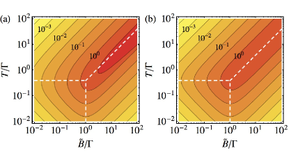
Figure 2: Temperature and magnetic field dependence of the spin-Seebeck coefficient (in units of $k_{B}/\left|e\right|$) of a noninteracting quantum dot. The maxima at $\tilde{B}=\Gamma$, $T=0.34\Gamma$ and $T=0.34\tilde{B}$ are indicated with dashed lines. (a) Exact result, Eq. (11). (b) Interpolation formula, Eq. (17).

In the absence of interaction the impurity Green’s function is $G_{\sigma}\left(\omega\right)=1/\bigl{(}\omega-\sigma\tilde{B}+i\Gamma\bigr{)}$. We introduced the energy level shift $\tilde{B}$ due to the magnetic field. In the non-interacting case, $\tilde{B}=\frac{B}{2}$. From Eqs. (7) and (10)

$$S_{s}={\cal S}\bigl{(}\tilde{B}\bigr{)}-{\cal S}\bigl{(}-\tilde{B}\bigr{)}=2{\cal S}\bigl{(}\tilde{B}\bigr{)}.$$ (11)

For $T\ll\max\left(\Gamma,\tilde{B}\right)$ the spin-Seebeck coefficient is proportional to the temperature,

$$S_{s}=\frac{4\pi^{2}}{3}\frac{\tilde{B}T}{\tilde{B}^{2}+\Gamma^{2}},$$ (12)

a results which can also be derived by performing the Sommerfeld expansion of the transport integrals in Eq. (6). It increases linearly with the field in low magnetic fields, $\tilde{B}\ll\Gamma$,

$$S_{s}=\frac{4\pi^{2}}{3}\frac{\tilde{B}T}{\Gamma^{2}},$$ (13)

and is inversely proportional to the field in high magnetic fields, $\tilde{B}\gg\Gamma$,

$$S_{s}=\frac{4\pi^{2}}{3}\frac{T}{\tilde{B}}.$$ (14)

It reaches its maximal value at $\tilde{B}=\Gamma$.

For $\tilde{B}\ll\max\left(\Gamma,T\right)$ the spin-Seebeck coefficient is proportional to the magnetic field:

$$S_{s}=\frac{2\tilde{B}}{T}\left(1+\frac{\Gamma}{2\pi T}\frac{\psi^{\prime\prime}\left(\frac{1}{2}+\frac{\Gamma}{2\pi T}\right)}{\psi^{\prime}\left(\frac{1}{2}+\frac{\Gamma}{2\pi T}\right)}\right).$$ (15)

In the low temperature limit, $T\ll\Gamma$, where we recover Eq. (13), it increases linearly with the temperature, reaching its maximal value at $T=0.34\Gamma$. It is inversely proportional to the temperature in the $T\gg\Gamma$ limit:

$$S_{s}=\frac{2\tilde{B}}{T}.$$ (16)

As shown in Fig. 2, an approximation that smoothly interpolates between the regimes of Eqs. (13), (14) and (16),

$$S_{s}^{-1}=\left(\frac{4\pi^{2}}{3}\frac{\tilde{B}T}{\Gamma^{2}}\right)^{-1}+\left(\frac{4\pi^{2}}{3}\frac{T}{\tilde{B}}\right)^{-1}+\left(\frac{2\tilde{B}}{T}\right)^{-1},$$ (17)

is qualitatively correct also at $\tilde{B},T\sim\Gamma$. According to this interpolation formula, the spin-Seebeck coefficient at $\tilde{B}=\Gamma$, $T=0.34\Gamma$ where the maxima merge is $S_{s}=1.45$, which compares well with the exact result of Eq. (11), $S_{s}=1.61$. From this point, the high spin-Seebeck coefficient ridge of $S_{s}\sim 1$ continues to higher temperatures and fields along the $T=0.34\tilde{B}$ line. Note also that at the ridge the magnetic field and the temperature are of the same order of magnitude.

Away from the particle-hole symmetric point, $\boldsymbol{\delta\neq 0}$

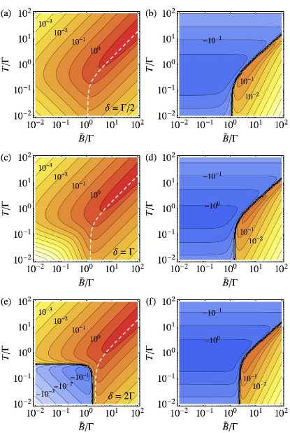
Figure 3: Temperature and magnetic field dependence of the spin-Seebeck coefficient (in units of $k_{B}/\left|e\right|$) of a noninteracting quantum dot away from the particle-hole symmetric point for (a) $\delta=\Gamma/2$, (c) $\delta=\Gamma$ and (e) $\delta=2\Gamma$. The corresponding electrical voltages, $-eV/\Delta T$, required for electrical current to vanish are shown in (b), (d) and (f). Along the dashed lines in (a), (c) and (e) the required electrical voltage is zero.

Here the spin-Seebeck coefficient, Eq. (8),

$$S_{s}={\cal S}\bigl{(}\delta+\tilde{B}\bigr{)}-{\cal S}\bigl{(}\delta-\tilde{B}\bigr{)},$$

and the electrical voltage required for the electrical current to vanish, Eq. (9),

$$-\frac{eV}{\Delta T}={\cal S}\bigl{(}\tilde{B}+\delta\bigr{)}-{\cal S}\bigl{(}\tilde{B}-\delta\bigr{)},$$

can also be related to the Seebeck coefficient of the spinless problem, Eq. (10).

In Figs. 3(a), (c) and (e) the spin-Seebeck coefficient $S_{s}$ is plotted for various values of the asymmetry parameter $\delta$. For $\delta<\Gamma$ the spin-Seebeck coefficient qualitatively resembles its $\delta=0$ behavior. At $\delta=\Gamma$ it is suppressed in the $\tilde{B},T\ll\Gamma$ region. For $\delta>\Gamma$ the spin-Seebeck coefficient becomes negative at low temperatures and fields. Its sign changes at $\tilde{B},T\sim\sqrt{\delta^{2}-\Gamma^{2}}$, as one can check by requiring ${\cal S}\bigl{(}\delta+\tilde{B}\bigr{)}={\cal S}\bigl{(}\delta-\tilde{B}\bigr{)}$ and using the approximate expression of Eq. (17) together with Eq. (11), ${\cal S}\left(\epsilon_{d}\right)=\frac{1}{2}\left.S_{s}\right|_{\tilde{B}\rightarrow\epsilon_{d}}$.

As evident from Figs. 3(b) (d) and (f), the electrical voltage required to stop the electrical current, $-eV/\Delta T$, can take both positive and negative values. At a given temperature this voltage is zero at a magnetic field $\tilde{B}$ where ${\cal S}\bigl{(}\tilde{B}+\delta\bigr{)}={\cal S}\bigl{(}\tilde{B}-\delta\bigr{)}$. This condition is fulfilled close to the point where the spin-Seebeck coefficient reaches a maximum as a function of the field, as shown with dashed lines in Figs. 3(a), (c) and (e).

V Method

To evaluate the transport integrals, Eq. (6), in the interacting case we employed the numerical renormalization group (NRG) methodWilson (1975); Krishna-murthy et al. (1980); Bulla et al. (2008). This method allows to compute the dynamical properties of quantum impurity models in a reliable and rather accurate way. The approach is based on the discretization of the continuum of bath states, transformation to a linear tight-binding chain Hamiltonian, and iterative diagonalization of this discretized representation of the original problem.

The Lehmann representation of the impurity spectral function isBulla et al. (2008)

$$\begin{split}A_{\sigma}\left(\omega\right)&=\frac{1}{Z}\sum_{p,r}\left(e^{-\frac{E_{p}}{T}}+e^{-\frac{E_{r}}{T}}\right)\times\\ &\times\left|\left\langle p\left|d_{\sigma}^{\dagger}\right|r\right\rangle\right|^{2}\delta\left(\omega-\left(E_{p}-E_{r}\right)\right).\end{split}$$

Here $p$ and $r$ index the many-particle levels $|p\rangle$ and $|r\rangle$ with energies $E_{p}$ and $E_{r}$, respectively. $Z$ is the partition function

$$Z=\sum_{p}e^{-\frac{E_{p}}{T}}.$$

This can also be expressed asYoshida et al. (2009); Seridonio et al. (2009)

$$\begin{split}A_{\sigma}\left(\omega\right)&=\frac{1}{Zf\left(\omega\right)}\sum_{p,r}e^{-\frac{E_{p}}{T}}\times\\ &\times\left|\left\langle p\left|d_{\sigma}^{\dagger}\right|r\right\rangle\right|^{2}\delta\left(\omega-\left(E_{p}-E_{r}\right)\right),\end{split}$$

where $f(\omega)$ is the Fermi-Dirac function. The transport integrals (6) are then calculated asYoshida et al. (2009); Seridonio et al. (2009)

$${\cal I}_{n\sigma} =\pi\frac{2\Gamma_{L}\Gamma_{R}}{\Gamma_{L}+\Gamma_{R}}\times$$

$$\times\frac{1}{ZT}\sum_{p,r}\left|\left\langle p\left|d_{\sigma}^{\dagger}\right|r\right\rangle\right|^{2}\frac{\left(E_{p}-E_{r}\right)^{n}}{e^{\frac{E_{p}}{T}}+e^{\frac{E_{e}}{T}}}.$$ (18)

In this approach it is thus not necessary to calculate the spectral function itself, thus the difficulties with the spectral function broadening and numerical integration do not arise. Furthermore, a single NRG run is sufficient to obtain the transport integrals in the full temperature interval. The calculations have been performed using the discretization parameter $\Lambda=2$, the truncation cutoff set at $12\omega_{N}$, and twist averaging over $N_{z}=8$ interleaved discretization meshes. The spin U(1) and the isospin SU(2) symmetries have been used to simplify the calculations.

An alternative approach for computing the transport integrals consists in calculating the spectral functions using the density-matrix NRG methodHofstetter (2000) or its improvements, the complete-Fock-space NRGAnders and Schiller (2005, 2006); Peters et al. (2006) or the full-density-matrix (FDM) NRG.Weichselbaum and von Delft (2007) In this case, a separate calculation has to be performed for each temperature $T$. The approaches based on the reduced density matrix are required to correctly determine the high-energy parts of the spectral function in the presence of the magnetic field.Hofstetter (2000) Nevertheless, since the main contribution to the transport integrals comes from the spectral weight on the low-energy scale of $\sim T$, which is well approximated even in the traditional approach,Oliveira and Wilkins (1981); Frota and Oliveira (1986); Sakai et al. (1989); Costi and Hewson (1992); Costi et al. (1994) there is little difference in the results obtained either way. We have explicitly calculated the spin thermopower for a set of parameters $B$ and $T$ using the FDM NRG and compared them against the results based on Eq. (18); the difference is smaller than the linewidth in the plot (a few percent at most), see Figs. 5(b) and 5(d). The FDM NRG is significantly slower than our approach because it requires one calculation for each value of $T$ and, furthermore, because each such calculation is significantly slower than a single calculation based on Eq. (18). The trade-off between an additional error of a few percent and an improvement in the calculation efficiency of more than two orders of the magnitude is well justified.

VI Results

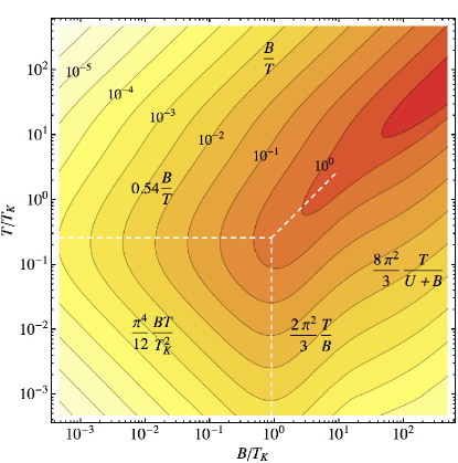
Figure 4: Temperature and magnetic field dependence of the spin-Seebeck coefficient (in units of $k_{B}/\left|e\right|$) as calculated with the NRG method. The positions of the maxima at $B=\frac{2\sqrt{2}}{\pi}T_{K}$, $T=0.26T_{K}$, and $T=0.29B$ are indicated with dashed lines.

We now turn to the numerical results for an interacting quantum dot. We choose a strongly correlated regime with $U=8\Gamma$. The Kondo temperature, Eq. (2), at the particle-hole symmetric point is then $T_{K}=0.11\Gamma$.

In Fig. 4 the spin-Seebeck coefficient is plotted for a range of temperatures and magnetic fields covering all the regimes of the symmetric Anderson model. It is evident from the Figure that for temperatures and magnetic fields at or above the Kondo temperature, but of roughly the same size, there is a ridge of high spin-Seebeck coefficient (of the order of $k_{B}/\left|e\right|$). At the point where the temperature and the field are both of the order of the Kondo temperature this ridge splits into two: one at the temperature of the order of the Kondo temperature with the spin-Seebeck coefficient decaying linearly as the field vanishes and the other at the magnetic field of the order of the Kondo temperature, again decaying linearly as the temperature vanishes. The ridges separate three slopes where the spin-Seebeck coefficient vanishes in directions away from the ridges.

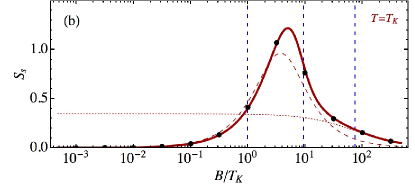
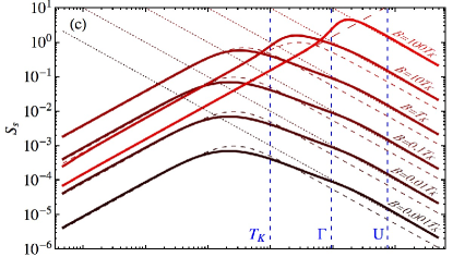
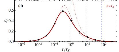
Figure 5: (a) Magnetic field dependence of the spin-Seebeck coefficient for several values of the temperature. The low magnetic field approximations are shown with dashed lines for $T=0.001T_{K}$, $T=0.01T_{K}$, $T=0.1T_{K}$ and $T=T_{K}$ [Eqs. (11) and (29)] and with long dashed lines for $T=10T_{K}$ and $T=100T_{K}$ [Eq. (28)]. The high magnetic field asymptotics, Eq. (25), are shown with dotted lines. (c) Temperature dependence for several values of the magnetic field. The low-temperature approximations are shown with dashed lines for $B=0.001T_{K}$, $B=0.01T_{K}$, $B=0.1T_{K}$, $B=T_{K}$ and $B=10T_{K}$ [Eqs. (11) and (29)] and with a long dashed line for $B=100T_{K}$ [Eq. (25)]. The high-temperature asymptotics, Eq. (28), are shown with dotted lines. In (b) and (d) the spin-Seebeck coefficient is presented in linear scale for $T=T_{K}$ and $B=T_{K}$, respectively. Black dots show the results obtained using the FDM NRG method.

We show that a treatment similar to that for a noninteracting quantum dot in Sec. IV is possible in the Kondo regime (and its vicinity) provided that we account for the temperature and field dependence of the position and the width of the Kondo resonance. On top of that we find simple asymptotic expressions for the spin thermopower far away from the Kondo regime. In Fig. 5(a) we compare these analytical results to the NRG data for various temperatures as a function of magnetic field on a log-log plot. In Fig. 5(b) one set of data is reproduced on a log-linear plot. In Figs. 5(c) and (d) we present such comparisons for various values of the magnetic field as a function of temperature. In the regions of their validity, the analytical expressions are found to reproduce the exact values reasonably well.

Particle-hole symmetric point, $\boldsymbol{\delta=0}$

We first study low temperature $T\ll\max\left(T_{K,}B\right)$ Fermi-liquid regimes and low magnetic field $B\ll\max\left(T_{K},T\right)$ regimes of the particle-hole symmetric model separately. Then we combine the results and present a unified theory which is capable of describing the spin thermopower at $B,T\sim T_{K}$.

Low-temperature regimes, $T\ll\max\left(T_{K,}B\right)$

Due to many-body effects there is an energy scale induced in the Anderson model which plays the role of an effective bandwidth. This energy scale is the Kondo temperature $T_{K}$ at low magnetic fields $B\ll T_{K}$ and rises up to $\Gamma$ as the magnetic field kills the Kondo effect. At temperatures low compared to this energy scale, i.e., in the Fermi-liquid regime, only the spectral function in the vicinity of the Fermi level is relevant to the calculation of the transport properties. Here the Green’s function can be parametrized in terms of the Fermi-liquid quasiparticle parameters, $G_{\sigma}\left(\omega\right)=z_{\sigma}/(\omega-\tilde{\varepsilon}_{d\sigma}+i\tilde{\Gamma}_{\sigma})$, where $z_{\sigma}=\left[1-\Sigma_{\sigma}^{\prime}\left(\mu\right)\right]^{-1}$ is the wavefunction renormalization factor, while $\tilde{\varepsilon}_{d\sigma}=z_{\sigma}\left[\varepsilon_{d}+\sigma\frac{B}{2}+\Sigma_{\sigma}\left(\mu\right)\right]$ and $\tilde{\Gamma}_{\sigma}=z_{\sigma}\Gamma$ are the quasiparticle energy level and its half-width, respectively.Hewson (1993) This parametrization provides an accurate description of the behavior of the system in the vicinity of the Fermi level, thus it is suitable for studying the transport properties; however, the features in the spectral function away from the Fermi level are not well described.

The spin-Seebeck coefficient is derived by performing the Sommerfeld expansion of the transport integrals in Eq. (7), resulting in the spin analog to the Mott formula,

$$S_{s}=\frac{2\pi^{2}}{3}\frac{A_{\uparrow}^{\prime}\left(0\right)}{A_{\uparrow}\left(0\right)}T=\frac{4\pi^{2}}{3}\frac{\tilde{\varepsilon}_{d\uparrow}T}{\tilde{\varepsilon}_{d\uparrow}^{2}+\tilde{\Gamma}_{\uparrow}^{2}}.$$ (19)

In the strong coupling regime, $B\ll T_{K}$, the quasiparticle level is shifted away from the chemical potential, $\tilde{\varepsilon}_{d\sigma}=\sigma\frac{B}{2}R$, where the Wilson ratio is $R=2$ due to residual quasiparticle interactionHewson et al. (2006) while its half-width is of the order of the Kondo temperature, $\tilde{\Gamma}_{\sigma}=\frac{4}{\pi}T_{K}$.Yamada (1975a, b) Thus the spin-Seebeck coefficient in the $B\ll T_{K}$ and $T\ll T_{K}$ regime increases linearly with both the temperature and the magnetic field:

$$S_{s}=\frac{\pi^{4}}{12}\frac{BT}{T_{K}^{2}}.$$ (20)

In the intermediate regime, $T_{K}\lesssim B\ll U$, the magnetic moment is localized but, due to strong logarithmic corrections, the field dependence of $\tilde{\epsilon}_{d\sigma}$ and $\tilde{\Gamma}_{\sigma}$ is nontrivial.Hewson et al. (2006) Anyway, a good agreement with numerical data is obtained for $B\lesssim\Gamma$ by allowing for the broadening of the quasiparticle level due to the magnetic field,Costi (2000); Andrei (1982)

$$\tilde{\Gamma}_{\sigma}^{2}=\left(\frac{4}{\pi}T_{K}\right)^{2}+B^{2},$$ (21)

and keeping the zero-field expression for the level shift, $\tilde{\epsilon}_{d\sigma}=\sigma B$:

$$S_{s}=\frac{4\pi^{2}}{3}\frac{BT}{2B^{2}+\left(\frac{4}{\pi}T_{K}\right)^{2}}.$$ (22)

This expression reaches its maximal value at $B=\frac{2\sqrt{2}}{\pi}T_{K}$. In the $T_{K}\ll B\ll\Gamma$ regime the spin-Seebeck coefficient is inversely proportional to the magnetic field:

$$S_{s}=\frac{2\pi^{2}}{3}\frac{T}{B}.$$ (23)

In the high magnetic field regime, $B\gtrsim U$, the Kondo resonance is no longer present and the Hubbard I approximation to the Green’s function may be used,Hubbard (1964)

$$G_{\text{$\sigma$}}\left(\omega\right)=\frac{1-\left\langle n_{d,-\sigma}\right\rangle}{\omega-\epsilon_{d}-\sigma\frac{B}{2}+i\Gamma}+\frac{\left\langle n_{d,-\sigma}\right\rangle}{\omega-\epsilon_{d}-U-\sigma\frac{B}{2}+i\Gamma},$$ (24)

where $\left\langle n_{d\sigma}\right\rangle$ is the occupation of the dot level with spin $\sigma$ electrons. In this regime, $\left\langle n_{d\downarrow}\right\rangle$ and $\left\langle n_{d\uparrow}\right\rangle$ approach 1 and 0, respectively, and $\tilde{\varepsilon}_{d\sigma}\approx\sigma\left(\frac{U}{2}+\frac{B}{2}\right)$, $\tilde{\Gamma}_{\sigma}=\Gamma$. The spin-Seebeck coefficient increases linearly with temperature, but is inversely proportional to the magnetic field for $B\gg U$:

$$S_{s}=\frac{8\pi^{2}}{3}\frac{T}{U+B}.$$ (25)

In Fig. 5 we compare this expression to the NRG data and find an excellent agreement in the appropriate regime.

Low magnetic field regimes, $B\ll\max\left(T_{K},T\right)$

At low and intermediate temperatures, $T\ll\Gamma$, only the Kondo resonance will play a role in determining the value of the spin-Seebeck coefficient. The effective dot level width, being equal to $\frac{4}{\pi}T_{K}$ at low temperatures, $T\ll T_{K}$, increases with temperature,Yamada (1975a, b)

$$\tilde{\Gamma}_{\sigma}^{2}=\left(\frac{4}{\pi}T_{K}\right)^{2}+\left(\pi T\right)^{2}.$$ (26)

Putting this expression, together with the low temperature expression for the level shift $\tilde{B}=B$, into the noninteracting quantum dot formula Eq. (15), we recover the Fermi-liquid asymptotic result Eq. (20) for $T\ll T_{K}$, while for $T\gg T_{K}$, as the width of the dot level becomes proportional to temperature, an asymptotic formula different from that of a noninteracting level, Eq. (16), results:

$$S_{s}=0.54\frac{B}{T}.$$ (27)

Between these asymptotic regimes the spin-Seebeck coefficient reaches its maximal value at $T=0.26T_{K}$.

In the free orbital regime, $T\gtrsim U$, the Hubbard I approximation, Eq. (24), can be used again. Now, due to high temperature $\left\langle n_{d\downarrow}\right\rangle=\left\langle n_{d\uparrow}\right\rangle\approx\frac{1}{2}$ and the effect of the magnetic field is only to shift the spectral functions,

$$\left.A_{\sigma}\left(\omega\right)\right|_{B}\to\left.A_{\sigma}\left(\omega-\sigma\frac{B}{2}\right)\right|_{B=0}.$$

As $-f^{\prime}\left(\omega\right)\approx\frac{1}{4T}$ in the region where the spectral density is appreciable, we get a simple expression

$$S_{s}=\frac{2}{T}\frac{\int\mathrm{d}\omega\omega\left.A_{\uparrow}\left(\omega-\frac{B}{2}\right)\right|_{B=0}}{\int\mathrm{d}\omega\left.A_{\uparrow}\left(\omega-\frac{B}{2}\right)\right|_{B=0}}.$$

Taking into account that in the absence of the magnetic field the spectral function is even, one can readily show that the spin-Seebeck coefficient is given by

$$S_{s}=\frac{B}{T},$$ (28)

thus recovering the non-interacting expression Eq. 16. In Fig. 5 we show that this expression correctly describes the asymptotic behavior of the spin-Seebeck coefficient in this regime.

Unified theory for $B,T\ll\Gamma$ regimes

Here the physics is governed by the Kondo resonance in the spectral function and its remnants at temperatures and magnetic fields above the Kondo temperature. A unified description of low and intermediate temperature and magnetic field regimes, $B,T\ll\Gamma$, is obtained using the noninteracting quantum dot spin-Seebeck coefficient formula, Eq. (11), and taking into account that the width of the Kondo resonance depends on both the temperature and the field. The appropriate phenomenological expression is a generalization of the low temperature, Eq. (26), and low magnetic field, Eq. (21), widths:

$$\tilde{\Gamma}_{\sigma}^{2}=\left(\frac{4}{\pi}T_{K}\right)^{2}+B^{2}+\left(\pi T\right)^{2}.$$ (29)

Again we use $\tilde{B}=B$. As evident in Fig. 5, this gives quite an accurate approximation, reproducing the correct position, width and, to a lesser extent, height of the peak in the spin-Seebeck coefficient. It becomes even more accurate for $U=16\Gamma$ (not shown here) where the Kondo energy scale is better separated from higher energy scales, resulting in a better agreement with the NRG data in the $B\lesssim T_{K}$ and $T_{K}\ll T\ll\Gamma$ regime.

At the point where the $B=\frac{2\sqrt{2}}{\pi}T_{K}$ and $T=0.26T_{K}$ maxima merge, the spin-Seebeck coefficient reaches a value of $S_{s}=0.53$, while the current approximation gives $S_{s}=0.63$. This universal value (provided the Kondo energy scale is well separated from higher energy scales, $T_{K}\ll\Gamma$) is somewhat lower than that of a noninteracting quantum dot which is a direct consequence of the widening of the Kondo energy level. From the merging point the spin-Seebeck coefficient increases only slightly, $S_{s}\sim 1$, along the $T=0.29B$ line.

As in the noninteracting case, Eq. (17), we can provide an analytical approximation for the spin-Seebeck coefficient by interpolating between the three asymptotic expressions of Eqs. (20), (23) and (27):

$$S_{s}^{-1}=\left(\frac{\pi^{4}}{12}\frac{BT}{T_{K}^{2}}\right)^{-1}+\left(\frac{2\pi^{2}}{3}\frac{T}{B}\right)^{-1}+\left(0.54\frac{B}{T}\right)^{-1}.$$ (30)

Away from the particle-hole symmetric point, $\boldsymbol{\delta\neq 0}$

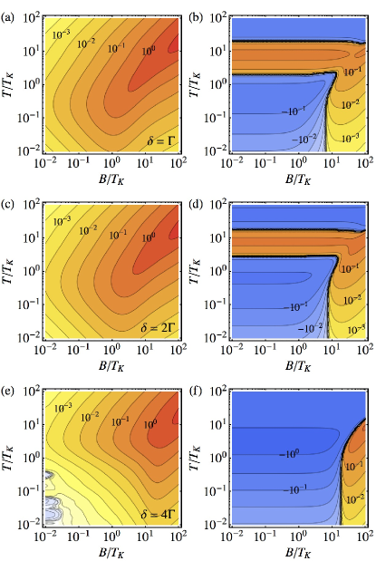
Figure 6: Temperature and magnetic field dependence of the spin-Seebeck coefficient (in units of $k_{B}/\left|e\right|$) as calculated with the NRG method away from the particle-hole symmetric point for (a) $\delta=\Gamma$, (c) $\delta=2\Gamma$ and (e) $\delta=4\Gamma$. The corresponding electrical voltages, $-eV/\Delta T$, required for electrical current to vanish are shown in (b), (d) and (f). Temperatures and magnetic fields are shown in units of the Kondo temperature in the particle-hole symmetric point. Note that because of the increase of the Kondo temperature with $\delta$, the maxima are shifted to higher temperature and magnetic field values. The low temperature and magnetic field structure in (e) is an artifact of the numerical method.

In Fig. 6 we present the spin-Seebeck coefficient for three different values of the asymmetry parameter $\delta$ ranging from the Kondo to the mixed valence regime. In the Kondo regime, $\delta=\Gamma=\frac{U}{8}$ in Fig. 6(a) and $\delta=2\Gamma=\frac{U}{4}$ in Fig. 6(b), the Kondo peak in the spectral function is pinned to the chemical potential in the absence of the magnetic field, $\tilde{\epsilon}_{d\sigma}\ll\tilde{\Gamma}_{\sigma}$.Hewson et al. (2004) The Kondo temperature increases with $\delta$, $T_{K}\propto\exp\left(\pi\delta^{2}/2U\Gamma\right)$,Hewson (1993) which causes the positions of maxima in the spin-Seebeck coefficient to shift to higher temperatures and fields. Provided we take this effect into account, the behavior of the spin-Seebeck coefficient reproduces that of the particle-hole symmetric situation in Fig. 4. In the mixed valence regime, $\delta=4\Gamma=\frac{U}{2}$ in Fig. 6(e), the Kondo peak has merged with the atomic peak resulting in a resonance in the spectral function of width $\tilde{\Gamma}_{\sigma}\sim\Gamma$ at $\tilde{\epsilon}_{d\sigma}\sim\tilde{\Gamma}_{\sigma}$ at $B=0$.Haldane (1978) The maxima shift to $T,B\sim\Gamma$ and we reproduce the characteristic suppression of the spin-Seebeck coefficient at low temperatures and fields observed in the noninteracting case in Fig. 3(c). In the empty orbital regime (not shown) the peak of width $\Gamma$ would shift even further away from the chemical potential and we would reproduce the noninteracting result of Fig. 3(e).

The electrical voltage required to stop the electrical current matches the prediction of the noninteracting theory in the mixed valence regime, Fig. 6(f), while in the Kondo regime, Figs. 6(b) and (d), it changes sign twice as a function of temperature at low magnetic fields. Such a behavior is consistent with the temperature dependence of the charge thermopower of a quantum dot studied by Costi and Zlatić in Ref. [Costi and Zlatić, 2010].

VII Summary

We demonstrated that the spin-Seebeck effect in a system composed of a quantum dot in a magnetic field, attached to paramagnetic leads, can be utilized to provide a pure spin current for spintronic applications provided the dot is held at the particle-hole symmetric point. By tuning the temperature and the field, the spin-Seebeck coefficient can reach large values of the order of $k_{B}/\left|e\right|$. Namely, for temperatures higher than $0.26T_{K}$, such a large spin thermopower is available at the magnetic field where $T=0.29B$. We carefully analyzed different regimes and derived analytical formulae which successfully reproduce and explain the temperature and magnetic field dependence of the spin-Seebeck coefficient calculated numerically with NRG.

Replacing the magnetic field with the gate voltage, the same conclusions are also valid for the charge thermopower of a negative-$U$ quantum dot, for which the charge-Seebeck coefficient of the order of $k_{B}/\left|e\right|$ was recently reported in Ref. [Andergassen et al., 2011].

We also studied the spin-Seebeck coefficient away from the particle-hole symmetric point. Our analysis shows that in the Kondo regime the results do not change qualitatively provided we take into account the increase of the Kondo temperature and apply a suitable electrical voltage across the dot to stop the electrical current.

As the Kondo temperature in quantum dots can be made quite low, the magnetic fields required to reach the large spin thermopower regime should be easily achievable in experiment.

Appendix A

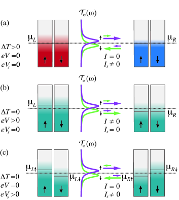
Figure 7: Currents generated by (a) temperature difference, (b) electrical voltage and (c) spin voltage applied across a quantum dot in a magnetic field $B>0$. The currents are shown separately for spin-up (violet arrows) and spin-down electrons (green arrows), as well as for electrons with energies higher (upper set of arrows) and lower (lower set of arrows) than the equilibrium chemical potential (black dotted line).

According to Eq. (3) the electrical current of spin $\sigma$ electrons is determined by the energy distribution of incoming electrons $f_{L\sigma}\left(\omega\right)-f_{R\sigma}\left(\omega\right)$ and the probability that those electrons are transmitted through the quantum dot ${\cal T}_{\sigma}\left(\omega\right)$. In the presence of a magnetic field, ${\cal T}_{\sigma}\left(\omega\right)$ is asymmetric about the chemical potential. Assuming the particle-hole symmetry and $B>0$ it is larger for spin-up electrons immediately above the chemical potential ($\omega>0$) than for those immediately below the chemical potential ($\omega<0$), and vice versa for spin-down electrons as ${\cal T}_{\downarrow}\left(\omega\right)={\cal T}_{\uparrow}\left(-\omega\right)$.

In the linear response regime we can study the effects of $\Delta T$, $eV$ and $eV_{s}$ separately as follows.

In the presence of a temperature difference $\Delta T$, Fig. 7(a), the energy distribution of the incoming electrons is the same for spin-up and spin-down electrons. For $\Delta T>0$ the incoming electrons with $\omega>0$ originate from the left (hot) lead while those with $\omega<0$ originate from the right (cold) lead. Now for $\omega>0$ there will be a surplus of spin-up electrons reaching the right lead due to the asymmetry of ${\cal T}_{\sigma}\left(\omega\right)$ while for $\omega<0$ the same surplus of spin-down electrons will reach the left lead, resulting in a zero electrical current and a finite spin current across the dot.

In the presence of an electrical voltage $eV>0$, Fig. 7(b), all the incoming electrons originate from the left lead, their energy distribution is an even function of $\omega$ and is again the same for both spin projections. For $\omega>0$ a surplus of spin-up electrons is reaching the right lead while for $\omega<0$ the same surplus of spin-down electrons is reaching the right lead. The result is a finite electrical current and a zero spin current.

In the presence of a spin voltage $eV_{s}>0$, Fig. 7(c), spin-up electrons originate from the left lead and spin-down electrons originate from the right lead. Energy distributions of the two species of incoming electrons, like the transmission probabilities ${\cal T}_{\sigma}\left(\omega\right)$, are related by reflection symmetry with respect to $\omega=0$. Consequently, the number of spin-up electrons reaching the right lead is the same as the number of spin-down electrons reaching the left lead, i.e. a zero electrical current and a finite spin current.

References

- Mahan et al. (1997) G. Mahan, B. Sales, and J. Sharp, Physics Today 50, 42 (1997).
- Segal (2005) D. Segal, Phys. Rev. B 72, 165426 (2005).
- Terasaki et al. (1997) I. Terasaki, Y. Sasago, and K. Uchinokura, Phys. Rev. B 56, R12685 (1997).
- Dubi and Di Ventra (2011) Y. Dubi and M. Di Ventra, Rev. Mod. Phys. 83, 131 (2011).
- Rejec et al. (2002) T. Rejec, A. Ramšak, and J. H. Jefferson, Phys. Rev. B 65, 235301 (2002).
- Scheibner et al. (2005) R. Scheibner, H. Buhmann, D. Reuter, M. N. Kiselev, and L. W. Molenkamp, Phys. Rev. Lett. 95, 176602 (2005).
- Costi and Zlatić (2010) T. A. Costi and V. Zlatić, Phys. Rev. B 81, 235127 (2010).
- Andergassen et al. (2011) S. Andergassen, T. A. Costi, and V. Zlatić, Phys. Rev. B 84, 241107 (2011).
- Uchida et al. (2008) K. Uchida, S. Takahashi, K. Harii, J. Ieda, W. Koshibae, K. Ando, S. Maekawa, and E. Saitoh, Nature 455, 778 (2008).
- Žutić et al. (2004) I. Žutić, J. Fabian, and S. Das Sarma, Rev. Mod. Phys. 76, 323 (2004).
- Datta and Das (1990) S. Datta and B. Das, Applied Physics Letters 56, 665 (1990).
- Wolf et al. (2001) S. A. Wolf, D. D. Awschalom, R. A. Buhrman, J. M. Daughton, S. von Molnár, M. L. Roukes, A. Y. Chtchelkanova, and D. M. Treger, Science 294, 1488 (2001).
- Wunderlich et al. (2010) J. Wunderlich, B.-G. Park, A. C. Irvine, L. P. Zârbo, E. Rozkotová, P. Nemec, V. Novák, J. Sinova, and T. Jungwirth, Science 330, 1801 (2010).
- Wang et al. (2010) R.-Q. Wang, L. Sheng, R. Shen, B. Wang, and D. Y. Xing, Phys. Rev. Lett. 105, 057202 (2010).
- Dubi and Di Ventra (2009) Y. Dubi and M. Di Ventra, Phys. Rev. B 79, 081302 (2009).
- Świrkowicz et al. (2009) R. Świrkowicz, M. Wierzbicki, and J. Barnaś, Phys. Rev. B 80, 195409 (2009).
- Ying and Jin (2010) Y. Ying and G. Jin, Applied Physics Letters 96, 093104 (2010).
- Lu et al. (2010) H.-F. Lu, L.-C. Zhu, X.-T. Zu, and H.-W. Zhang, Applied Physics Letters 96, 123111 (2010).
- Hewson (1993) A. Hewson, The Kondo Problem to Heavy Fermions (Cambridge University Press, New York, N.Y., 1993).
- Martinek et al. (2005) J. Martinek, M. Sindel, L. Borda, J. Barnaś, R. Bulla, J. König, G. Schön, S. Maekawa, and J. von Delft, Phys. Rev. B 72, 121302 (2005).
- Horvatic and Zlatic (1985) B. Horvatic and V. Zlatic, J. Phys. (France) 46, 1459 (1985).
- Meir and Wingreen (1992) Y. Meir and N. S. Wingreen, Phys. Rev. Lett. 68, 2512 (1992).
- Taraphder and Coleman (1991) A. Taraphder and P. Coleman, Phys. Rev. Lett. 66, 2814 (1991).
- Mravlje et al. (2005) J. Mravlje, A. Ramšak, and T. Rejec, Phys. Rev. B 72, 121403 (2005).
- Koch et al. (2007) J. Koch, E. Sela, Y. Oreg, and F. von Oppen, Phys. Rev. B 75, 195402 (2007).
- Abramowitz and Stegun (1964) M. Abramowitz and I. Stegun, Handbook of Mathematical Functions (Dover, New York, 1964), 5th ed.
- Wilson (1975) K. G. Wilson, Rev. Mod. Phys. 47, 773 (1975).
- Krishna-murthy et al. (1980) H. R. Krishna-murthy, J. W. Wilkins, and K. G. Wilson, Phys. Rev. B 21, 1003 (1980).
- Bulla et al. (2008) R. Bulla, T. Costi, and T. Pruschke, Rev. Mod. Phys. 80, 395 (2008).
- Yoshida et al. (2009) M. Yoshida, A. C. Seridonio, and L. N. Oliveira, Phys. Rev. B 80, 235317 (2009).
- Seridonio et al. (2009) A. C. Seridonio, M. Yoshida, and L. N. Oliveira, Phys. Rev. B 80, 235318 (2009).
- Hofstetter (2000) W. Hofstetter, Phys. Rev. Lett. 85, 1508 (2000).
- Anders and Schiller (2005) F. B. Anders and A. Schiller, Phys. Rev. Lett. 95, 196801 (2005).
- Anders and Schiller (2006) F. B. Anders and A. Schiller, Phys. Rev. B 74, 245113 (2006).
- Peters et al. (2006) R. Peters, T. Pruschke, and F. B. Anders, Phys. Rev. B 74, 245114 (2006).
- Weichselbaum and von Delft (2007) A. Weichselbaum and J. von Delft, Phys. Rev. Lett. 99, 076402 (2007).
- Oliveira and Wilkins (1981) L. N. Oliveira and J. W. Wilkins, Phys. Rev. B 24, 4863 (1981).
- Frota and Oliveira (1986) H. O. Frota and L. N. Oliveira, Phys. Rev. B 33, 7871 (1986).
- Sakai et al. (1989) O. Sakai, Y. Shimizu, and T. Kasuya, J. Phys. Soc. Jpn. 58, 3666 (1989).
- Costi and Hewson (1992) T. A. Costi and A. C. Hewson, Phil. Mag. B 65, 1165 (1992).
- Costi et al. (1994) T. A. Costi, A. C. Hewson, and V. Zlatić, J. Phys.: Condens. Matter 6, 2519 (1994).
- Hewson et al. (2006) A. C. Hewson, J. Bauer, and W. Koller, Phys. Rev. B 73, 045117 (2006).
- Yamada (1975a) K. Yamada, Prog. Theor. Phys. 53, 970 (1975a).
- Yamada (1975b) K. Yamada, Prog. Theor. Phys. 54, 316 (1975b).
- Costi (2000) T. A. Costi, Phys. Rev. Lett. 85, 1504 (2000).
- Andrei (1982) N. Andrei, Physics Letters A 87, 299 (1982).
- Hubbard (1964) J. Hubbard, Proc. Roy. Soc. (London) A283, 401 (1964).
- Hewson et al. (2004) A. Hewson, A. Oguri, and D. Meyer, The European Physical Journal B - Condensed Matter and Complex Systems 40, 177 (2004).
- Haldane (1978) F. D. M. Haldane, Phys. Rev. Lett. 40, 416 (1978).