Directional Variance Adjustment: improving covariance estimates for high-dimensional portfolio optimization

Abstract

Robust and reliable covariance estimates play a decisive role in financial and many other applications. An important class of estimators is based on Factor models. Here, we show by extensive Monte Carlo simulations that covariance matrices derived from the statistical Factor Analysis model exhibit a systematic error, which is similar to the well-known systematic error of the spectrum of the sample covariance matrix. Moreover, we introduce the Directional Variance Adjustment (DVA) algorithm, which diminishes the systematic error. In a thorough empirical study for the US, European, and Hong Kong market we show that our proposed method leads to improved portfolio allocation.

1 Introduction and Motivation

The advent of modern finance began with Markowitz and his seminal paper on portfolio optimization (Markowitz (1952)). His theory provides a mathematical approach to diversification by directly minimizing the portfolio variance. Moreover, by adding constraints to the optimization problem, we can e. g. prohibit or allow short-selling. Other applications comprises the creation of portfolios which constitute optimal hedges or track indices. However, a fundamental issue in portfolio allocation is the accurate and precise estimation of the covariance matrix of asset returns from historical data.

Covariance estimation and coping with its uncertainties have occupied both researchers and practitioners since then. One of the major difficulties with robust covariance matrix estimation arises from nonstationarity of financial time series (see, e.g. Loretan and Phillips (1994), Pagan and Schwert (1990)). Here, changes in the data generating processes force the estimation to rely on short time windows of recent observations. On the other hand the number of parameters increases quadratically with the number of assets, i.e., for a set of $N$ assets, the covariance matrix has $\frac{1}{2}N(N+1)$ free parameters. For example, in order to estimate the covariance matrix from daily return series of a moderately sized universe of one hundred assets, already 5050 free parameters have to be estimated. Following a general rule of thumb, that 10 observations per parameter are required for a reliable estimate, the observation window would need to cover approximately two years of data. Such a temporal horizon, however, clearly contradicts with reported nonstationarity of financial time series. In practice, the situation is even exacerbated by non-Gaussianity of financial time series (see, e.g., Loretan and Phillips (1994), Longin (2005), Campbell et al. (2008)), which increases the difficulty of covariance estimation even further, especially in case of small sample sizes. A possible remedy for problems caused by non-Gaussianity are robust estimation techniques (Huber (1981)).

As the terms high dimensional and small sample size are rather vague and interdependent, the difficulty of the task of covariance estimation is commonly characterized by the ratio of sample size to dimensionality, $T/N$, which governs the properties of the spectrum of the sample covariance matrix (Marčenko and Pastur (1967); Edelman and Rao (2005)). For situations where this ratio is close to one or even below, many estimators which give better results than the sample covariance matrix have been proposed. Here, an important class is formed by regularized estimators, in which the effective degrees of freedom are reduced by shrinkage (see, e. g., Stein (1956); Friedman (1989); Ledoit and Wolf (2003); Schäfer and Strimmer (2005)). Another way to reduce the degrees of freedom is to impose a latent structure on the data. Here, commonly factor models (FMs) are in use. FMs assume the data to be generated as a mixture of a small number of factors with additive noise (Fan et al. (2008), Goldfarb and Iyengar (2003)).

In this paper, we will analyse a purely statistical factor model called (Maximum Likelihood) Factor Analysis (see, e. g., Basilevsky (1994)). As there is no analytic solution for the parameters of the Factor Analysis model, we cannot provide a stringent theoretic analysis of its properties. Instead, by means of thorough simulations, we will provide evidence that the spectrum of the covariance matrix derived from a Factor Analysis model is biased. To reduce the bias, we will propose the Directional Variance Adjustment (DVA) algorithm, which estimates the magnitude of the imposed bias in specific directions by means of a Monte Carlo sampling approach and hence enables for its correction.

In the portfolio optimization literature Monte Carlo sampling is known from Resampling Efficiency (Michaud (1998)). There, the authors follow a fundamentally different approach. While we use resampling to reduce the bias of our factor model, in Resampling Efficiency the sample mean and covariance are used to generate additional data sets, on which optimal portfolio weights are calculated which are then averaged. This is supposed to lead to more stable and diversified portfolios, but there is an ongoing debate on the merits of this procedure (see, e.g. Scherer (2004)). Though not based on Monte Carlo resampling, techniques for the correction of variance inflation in principal components analysis are more related to our algorithm (Kjems et al. (2001); Abrahamsen and Hansen (2011)).

At this point we would like to emphasize that in this paper we will solely focus on the structure of risk in the stock market. A discussion about the structure of expected returns (see, e. g. $\beta$-pricing models, Shanken (1992)) is not within the scope of the paper.

We will evaluate our novel covariance estimation procedure in the context of portfolio optimization, where we will compare the proposed DVA Factor Analysis model to the sample covariance, Resampling Efficiency, Shrinkage, standard Factor Analysis and the Fama-French Three-Factor model (Fama and French (1992)). By means of analyzing daily return data from 2001–2009 of three different markets, namely the US, EU and Hong Kong stock markets, we will show that our proposed covariance matrix estimation scheme leads to an improved portfolio allocation and hence provide evidence that it better reflects the market’s risk structure.

The paper is organized as follows. Section 2 reviews covariance estimation methods. In section 3, we will review Factor Analysis and investigate the bias in Factor Analysis by means of simulated data. Then, we will introduce our novel DVA approach for dealing with the systematic error in the model and show the effectiveness in additional simulations. In Section 4 we will present the results of a thorough comparative study of various covariance estimation methods in the context of portfolio optimization. Section 5 concludes the paper.

2 Covariance Estimation

2.1 Sample Covariance Matrix and Systematic Error in its Spectrum

The sample covariance matrix,

$$C^{sc}_{ij}=\frac{1}{T-1}\sum^{T}_{t=1}(r_{ti}-\bar{r_{i}})\cdot(r_{tj}-\bar{r_{j}}),$$ (1)

where $\mathbf{R}$ is the ($T\times N$)-matrix containing $T$ observations of $N$ variables, is a consistent estimator of the covariance matrix. This means that for $T\rightarrow\infty$ the sample covariance matrix converges to the true covariance matrix. When the ratio T/N is not large, however, the sample covariance matrix tends to be ill-conditioned, implying that its inverse incurs large errors. In the extreme case, when the number of observations falls below the number of variables, the covariance matrix gets singular.

Though the sample covariance is an unbiased estimator of the true covariance matrix, this estimator exhibits a systematic misestimation of the spectrum of the covariance matrix which depends on the ratio of observations to dimensionality $T/N$. In particular, large and small Eigenvalues are systematically over- and underestimated, respectively (see, e. g. Friedman (1989)). In order to illustrate this systematic error, we generated empirical spectra from the Marčenko-Pastur density of eigenvalues for i.i.d. standard normally distributed variables (Marčenko and Pastur (1967)). The Marčenko-Pastur density is the eigenvalue density in the limit $T,N\rightarrow\infty$, but already for sample sizes as small as 20 or 30 the empirical distribution is very similar (Tulino and Verdú (2004)). Figure 1 shows the analytical solution for the empirical spectra for various ratios of sample sizes to dimensionality. The magnitude of the systematic error scales with the inverse of this ratio, for the degenerate case ($T/N<1$) there are $N-T$ zero eigenvalues. Even for $T/N=100$, the spectrum still differs visibly from the true one.

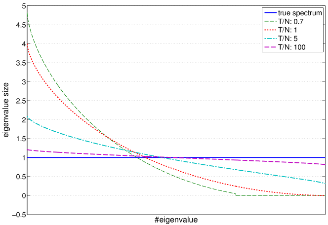
Figure 1: Systematic error in the estimated eigenvalues of the sample covariance matrix for different ratios of sample size to dimensionality.

Several methods have been proposed in the literature for correcting the spectrum. In Shrinkage (Ledoit and Wolf (2003, 2004); Schäfer and Strimmer (2005)), the goal is to find a suitable convex combination of the sample covariance matrix $\mathbf{C}^{sc}$ and a shrinkage target $\mathbf{C}^{target}$,

$$\mathbf{C}^{sh}=\lambda\mathbf{C}^{sc}+(1-\lambda)\mathbf{C}^{target},$$ (2)

where the shrinkage target is either fixed (e. g. $\mathbf{C}^{target}=\mathbf{I}$) or a biased estimator with lower variance (e. g. all correlations set to their average value). For selecting the optimal shrinkage strength $\lambda$, Ledoit and Wolf (2004) proposed an analytic solution, which is computationally faster than the commonly used model selection via crossvalidation. Shrinkage can be combined with factor modelling by taking a factor model as the shrinkage target (Ledoit and Wolf (2003)).

Random Matrix Theory (RMT, for an overview see Edelman and Rao (2005)) allows for several alternative approaches to correct the spectrum. Rosenow et al. (2002) propose to retain only those eigenvalues of the correlation matrix which are larger than the largest eigenvalues of a random matrix, given by the Marčenko-Pastur law, and therefore likely to reflect some real structure. The model itself is equivalent to a PCA factor model based on the correlation matrix, where RMT is used for selection of the appropriate number of factors. A similar model is proposed by Laloux et al. (2000). Instead of setting the eigenvalues in the bulk of the spectrum to zero, they are set to their average value. A detailed analysis of these methods is beyond the scope of this article. Note that these methods are closely related to the PCA and the FA factor model which we will discuss. Thus, these models exhibit a similiar performance and suffer from the same bias we discuss in the following.

An interesting approach is described in el Karoui (2008). There, the Marčenko-Pastur law which describes the distribution of the sample eigenvalues is inverted numerically in order to obtain the true spectrum from the sample. For this, one has to be aware of two facts: first, the inversion is not unique and therefore a prior or parametric ansatz has to be applied. Second, the largest eigenvalue of the covariance matrix of asset returns is normally isolated from the bulk. This is problematic, because the inversion leads to a continous spectrum. These aspects make the application of this approach less straightforward and, to our knowledge, no publication with portfolio simulations exists in which a competetive performance was achieved.

The following section introduces Factor Models as a type of restricted covariance estimator.

2.2 Factor Models as Restricted Covariance Estimators

In finance, factor models form an important class of restricted covariance estimators. In a factor model, the returns $r_{ti}$ of the $i^{\mbox{\tiny th}}$ asset at time $t$ are described as a weighted sum of $M$ random factor returns $f_{tm}$ multiplied with exposures $X_{mi}$ to these factors and additional random noise $e_{ti}$:

$$r_{ti}=\; \underbrace{\sum_{m=1}^{M}f_{tm}\cdot X_{mi}}_{systematic\;risk}\quad+\underbrace{\;\;\;e_{ti}\;\;}_{specific\;risk}$$ (3)

$$e_{i}{\perp\!\!\!\perp}f_{j},\qquad\forall\;i,j$$

$$e_{i}{\perp\!\!\!\perp}e_{j},\qquad\forall\;i\neq j.$$

Here, the systematic risk entirely describes the dependencies between the assets, while the asset specific risks are assumed to be independent.

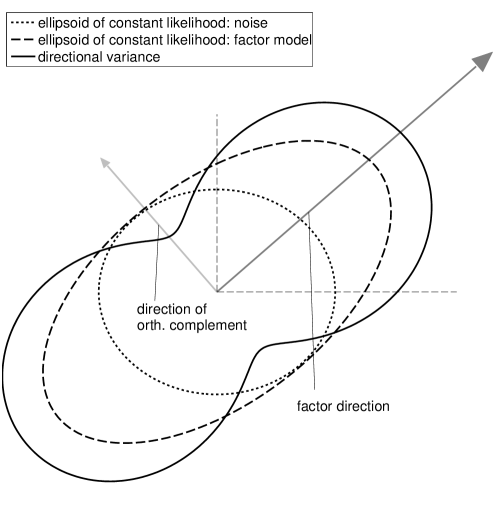
Figure 2: A two dimensional example of a $1$-factor model. The arrows show the direction of the single factor and the orthogonal complement. The covariance matrices of the factor model $\mathbf{C}^{fm}$ (dashed) and the uncorrelated noise $\mathbf{\Sigma}_{e}$ (dotted) are shown as ellipsoids of constant likelihood. The peanut-shaped solid line shows the directional variances (${\bf v}^{\top}\mathbf{C}^{fm}{\bf v}$) of the factor model along all directions ${\bf v}:\lVert{\bf v}\rVert_{2}=1$.

In the statistics and signal processing literature, this is often referred to as a mixture model, where $\mathbf{X}$ is the mixture matrix and $\mathbf{f}$ are the source signals (see, e. g.,Hyvärinen and Oja (2000). Calculating the covariance matrix, one obtains

$$\mathbf{C}^{fm}=\mathbf{R}^{\top}\mathbf{R}= \mathbf{(FX)}^{\top}\mathbf{(FX)}+\mathbf{E}^{\top}\mathbf{E}$$

$$= \mathbf{X}^{\top}\mathbf{\Sigma}_{f}\mathbf{X}+\mathbf{\Sigma}_{e},$$ (4)

where $\mathbf{\Sigma}_{f}$ is the covariance of the factors and the diagonal matrix $\mathbf{\Sigma}_{e}$ is formed by the asset specific noise variances (cf. Figure 2).

The advantage of factor models lies in the reduced number of parameters for covariance estimation. Essentially, this means that a higher bias is accepted in exchange for a reduced variance. In quantitative finance, three different types of factors are employed to build up factor models: fundamental, macroeconomic and statistical factors (Connor (1995); Gregory et al. (2010)).

In a fundamental factor model, assets are analysed and certain key metrics are used for setting up the factor model. Fundamental factor models are especially well suited when only a short history of data is available, e. g. for weekly or monthly data, as fewer parameters have to be estimated from the history than in a statistical factor model. The best-known model of this kind is the Fama-French three-factor model (Fama and French (1992)), in which the factor time series $\mathbf{f}$ are based on portfolios governed by market beta, book-to-market ratio and market capitalization. The exposures to these factors are obtained from the coefficients of a linear regression model.

In contrast, macroeconomic factor models predetermine the factors as macroeconomic time series which are supposed to affect the asset returns. As in the Fama-French model, the exposures are obtained by linear regression. Examples for macroeconomic time series used in factor models are unemployment rate, GNP, FX or interest rates. However, for daily or higher frequency stock market returns, macroeconomic factor models are of limited use and therefore neglected in the following (for an overview, see Gregory et al. (2010)).

The third approach, statistical factor modelling, is purely data driven and extracts the factors as well as the exposures from historical asset time series. Representatives of statistical factor models are Principal Component Analysis (PCA, Jolliffe (1986)), Probabilistic Principal Component Analysis (PPCA, Tipping and Bishop (1999)), Independent Component Analysis (ICA, Comon (1994); Hyvärinen and Oja (2000)) as well as Factor Analysis (FA, see section 3.1).

Hybridization allows for models which combine statistical, fundamental and/or macroeconomic factors (Connor (1995); Miller (2006); Gregory et al. (2010)). As long as the hybrid models contain statistical factors, our approach could be adapted to improve covariance estimation.

3 Directional Variance Adjustment of Factor Analysis

3.1 (Maximum Likelihood) Factor Analysis

Factor Analysis is a latent variable model which has its roots in psychology and answers the question for the ”best” explanation of the observed data for a given number of factors (latent variables). Here, ”best” model refers to the model that maximizes the data likelihood. The application of Factor Analysis to financial data was first introduced in order to test the Arbitrage Pricing Theory (Roll and Ross (1980)).

Factor Analysis models the asset returns as a mixture of unobserved source signals with additive noise. The signals and the noise are assumed to be i.i.d., zero-mean normally distributed. Independence of the noise ($\rightarrow$ diagonal noise covariance matrix) and independence of noise and factors ($\rightarrow$ covariance is a sum of factor and noise contributions) are assumed (cf. eq. (3)). In addition, it is assumed that scaling and correlation of the systematic risk are contained in the mixing matrix ($\rightarrow$ standard normally distributed independent factors). Hence, the model reads as

$$\mathbf{r}_{t}= \mathbf{f}_{t}\cdot\mathbf{X}+\boldsymbol{\epsilon}_{t},$$ (5)

$$\mathrm{with}\qquad\mathbf{f}_{t}\sim{\cal N}(0,\mathbf{I}), \quad\quad\boldsymbol{\epsilon}_{t}\sim{\cal N}(0,\mathbf{D}),$$

where $\mathbf{D}$ is a diagonal matrix. The corresponding log-likelihood is obtained as

$$L(\mathbf{X},\,\mathbf{D})=\ln p(\mathbf{R},\,\mathbf{F}|\mathbf{X},\,\mathbf{D}) = \sum_{t=1}^{T}\left\{\ln p(\mathbf{r}_{t}|\mathbf{f}_{t},\mathbf{X},\,\mathbf{D})+\ln p(\mathbf{f}_{t})\right\}.$$ (6)

Especially in the finance context, normality is a strong assumption. In order to make the model more appropriate for financial data, it is possible to extend FA to t-distributions (t-FA, see McLachlan et al. (2007)). t-FA has the same bias as standard FA and our method can be adapted in a straightforward way by replacing FA by t-FA, but a comparison of these methods is beyond the scope of this paper.

We obtain estimates of the model parameters by Expectation-Maximization (EM, see Dempster et al. (1977), for applications on Factor Analysis see Rubin and Thayer (1982) and Roweis and Ghahramani (1999)). In this algorithm, the likelihood is maximized iteratively by alternating between the Expectation and the Maximization step:

• in the Expectation step, the exposure $\mathbf{X}$ and noise variance $\mathbf{D}$ are assumed to be fixed and the expected factor $\mathbf{F}$ (latent variables) can be derived directly.

• in the Maximization step, the expected factors $\mathbf{F}$ are assumed to be fixed and the likelihood is maximized with respect to exposures $\mathbf{X}$ and noise variances $\mathbf{D}$.

These two steps are iterated until convergence. The resulting covariance matrix estimate of the Factor Analysis model is then given as

$$\hat{\mathbf{C}}^{fa}=\mathbf{\hat{X}}^{\top}\mathbf{\hat{X}}+\mathbf{\hat{D}}.$$ (7)

Note that the above equation follows trivially from eq. (4) for independent and standard normal factors. For Factor Analysis the number of parameters is reduced from $\frac{1}{2}N(N+1)$ to

$$df= \;\underbrace{M\cdot N}_{entries\,in\,X}\quad-\underbrace{\;(M-1)\;}_{rotational\,invariance\,of\,X}\quad+\underbrace{\;\;N\;}_{diagonal\,elements\,of\,D}$$

$$= \;(M+1)\cdot(N-1)+2.$$ (8)

3.2 Systematic Error in Factor Analysis

Since there are no analytical results for the spectrum of Factor Analysis as there are for the sample covariance matrix (section 2.1), we run a simulation to study systematic errors in Factor Analysis. To this end, we generate $N=30$ dimensional return data according to an underlying three factor model as in eq. (5). The noise covariance matrix $\mathbf{D}$ was defined with equally spaced values from the intervall $[0.5,1.5]$ on the diagonal. The three rows of the mixing matrix $\mathbf{X}$ were generated as randomly oriented vectors with a length of 10, 3 and 1, respectively. In order to study the small sample size properties of Factor Analysis for this setting, we set the ratio $T/N$ to 0.7, 1 and 5, corresponding to 21, 30, and 150 thirty-dimensional observations. As $\mathbf{X}$ and $\mathbf{D}$ are known for the simulation, the true covariance matrix $\mathbf{C}^{true}$ can be calculated by the population counterpart of eq. (7).

In section 2.1 we studied the systematic error of the eigenspectrum of the sample covariance matrix, where the variance in the $i$-th eigendirection $\mathbf{v}_{i}$ corresponds to the size of the $i$-th eigenvalue $\lambda_{i}$:

$$\mathbf{v}_{i}^{\top}\mathbf{C}\mathbf{v}_{i}=\mathbf{v}_{i}^{\top}\lambda_{i}\mathbf{v}_{i}=\lambda_{i}.$$

In the following we will study systematic errors in terms of misspecification of directional variances. More precisely, we will investigate systematic errors in the factor subspace and its complementary orthogonal space separately. To this end we first calculate an orthonormal basis $\mathbf{P}^{0}_{fs}$ ($N\times M$) of the $M$-dimensional subspace in which the estimated factors ${\mathbf{\hat{X}}}$ lie (the Factor Subspace) and another orthonormal basis $\mathbf{P}^{0}_{oc}$ ($N\times(N-M)$) of the $(N-M)$-dimensional orthogonal complement. Correspondingly, we can confine the covariance matrix to the two subspaces, yielding a factor space related part and its orthogonal counterpart as

$$\mathbf{C}^{fa}_{fs}:= \;\mathbf{P}^{0}_{fs}{\mathbf{P}^{0}_{fs}}^{\top}\mathbf{C}^{fa}\mathbf{P}^{0}_{fs}{\mathbf{P}^{0}_{fs}}^{\top}\qquad\qquad\mathrm{and}$$

$$\mathbf{C}^{fa}_{oc}:= \;\mathbf{P}^{0}_{oc}{\mathbf{P}^{0}_{oc}}^{\top}\mathbf{C}^{fa}\mathbf{P}^{0}_{oc}{\mathbf{P}^{0}_{oc}}^{\top}.$$

For each subspace, we obtain a new basis ($\mathbf{P}_{fs}$ and $\mathbf{P}_{oc}$) as the corresponding eigenbasis of $\mathbf{C}^{fa}_{fs}$ and $\mathbf{C}^{fa}_{oc}$, respectively. Combining these subspace bases to $\mathbf{P}$ = [$\mathbf{P}_{fs}$,$\mathbf{P}_{oc}$] yields an orthonormal basis of the entire space ($\mathbb{R}^{N}$).

Along these directions $\mathbf{p}_{i}$ we measure the directional variances $\sigma_{i}^{2}$ for the true and the estimated Factor Analysis model and calculate the systematic error as

$$S^{fa}_{i}=\mathbb{E}\left[\frac{\sigma^{2\,fa}_{i}}{\sigma^{2\,true}_{i}}\right],\qquad\sigma^{2\,true}_{i}=\mathbf{p}_{i}^{\top}\mathbf{C}^{true}\mathbf{p}_{i}\ ,\qquad\sigma^{2\,fa}_{i}=\mathbf{p}_{i}^{\top}\mathbf{C}^{fa}\mathbf{p}_{i}.$$ (9)

Here, values $S_{i}>1$ and $S_{i}<1$ correspond to an over- and underestimation of the directional variances, respectively. Moreover, the basis $\mathbf{P}$ explicitly takes the factor structure into account. Hence, this particularly chosen basis enables us to study the specific systematic estimation errors in the factor subspace and noise subspace separately. Note that the directions $\mathbf{p}_{i}$ are solely derived from the estimated parameters of the factor model and do not rely on information about the true covariance matrix.

Figure 3 depicts the estimated systematic error $S$ (eq. (9)) of Factor Analysis by means of the simulated data. Clearly, Factor Analysis tends to overestimate the variance in the $3$-dimensional Factor Subspace, while the variance in the orthogonal complement is on average underestimated. This is not surprising, as the Factor Analysis model attributes strong covariances in the sample to the factors. Consequently, factors with low Signal-to-Noise-ratio (SNR) are hard to identify and directions of spurious covariance are likely to be misrepresented as factors, yielding an overestimating of the variance along these directions: In the simulations, the strongest (first) factor, which has a high Signal-to-Noise-Ratio can be estimated with very high accuracy even for small sample sizes and the variance estimate does not have a significant systematic error. The weaker factors with a lower SNR in contrast tend to yield overestimated variances along the estimated factor directions. This effect is highly pronounced for small sample sizes and persists for relatively large sample sizes.

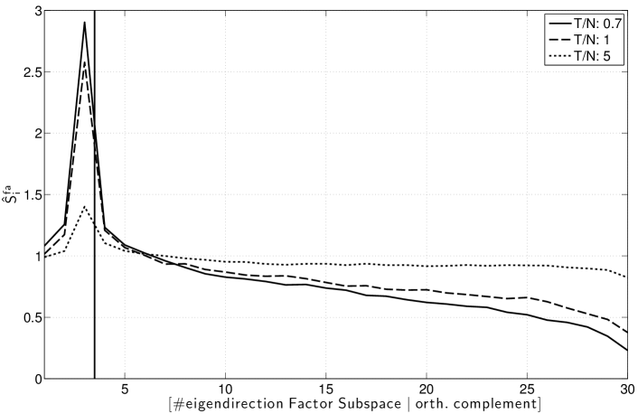
Figure 3: average ratio between Factor Analysis and true variances in the factor subspace and the orthogonal complement. Ratios of sample size to dimensionality $T/N=0.7$, $1$ and $5$. $N=30$. Average over 150 datasets.

On the other hand, the noise subspace spectrum shows a similar – albeit weaker – behaviour as the spectrum of the sample covariance matrix, i.e., variances corresponding to large eigenvalues are overestimated, while variances corresponding to small eigenvalues are underestimated (compare Figure 1 and Figure 3). As for the sample covariance matrix, this effect is especially pronounced for small sample sizes.

3.3 Directional Variance Adjustment: Correcting the Systematic Error

The systematic error of the spectrum of a sample covariance matrix with respect to the true spectrum can be estimated analytically: from the distribution of the entries in the covariance matrix, the distribution of the eigenvalues can be derived (see e.g., Edelman and Rao (2005)). The minimization of the Factor Analysis cost function on the other hand does not have a closed form solution, an iterative method has to be used. Hence it does not facilitate an analytical approach to obtain the distribution of the eigenvalues. Consequently, we will deploy a method that is based on Monte-Carlo-sampling.

To this end, suppose we have estimated the parameters $\cal{F}$ of a Factor Analysis model and want to correct the corresponding covariance matrix $\mathbf{C}^{\cal{F}}$ for the systematic error. Then we estimate the systematic error in the following manner: Using ${\cal{F}}$ for a generative model, we generate $K$ synthetic data sets of the same size as the original sample. For each data set we estimate a corresponding Factor Analysis parameter set ${\cal{F}}_{1},\dots,{\cal{F}}_{K}$. Note that for these parameter sets the true set of parameters (i.e., $\cal{F}$) is known and with it the true covariance matrix. This enables us to quantify the amount by which the directional variances along the eigendirections of $\mathbf{C}_{fs}^{{\cal F}_{k}}$ (factor subspace) and $\mathbf{C}_{oc}^{{\cal F}_{k}}$ (orthogonal complement) are over- and underestimated, respectively. The estimated systematic errors, can then directly be turned into multiplicative correction factors for the adjustment of the directional variances of $\cal{F}$. Applying these corrections to the eigendirections of the factor space and its orthogonal complement yields to what we refer as the directional variance adjusted covariance matrix $\mathbf{C}^{DVA}$ of $\cal{F}$ (see algorithm 1).

Algorithm 1 DVA

0:  the estimated parameters of the Factor Analysis model $\cal{F}$ ; the sample size $T$; the number of Monte Carlo runs $K$

0:  the directional variance adjusted covariance $\mathbf{C}^{DVA}$

1:  generate $K$ synthetic data sets of size $T$ based on $\cal{F}$.

2:  from the $K$ data sets, estimate $K$ factor model parameter sets ${\cal{F}}_{1},\dots,{\cal{F}}_{K}$

3:  For each ${\cal{F}}_{k}$, estimate the basis $\mathbf{P}_{k}$ = [$\mathbf{P}_{k,fs}$,$\mathbf{P}_{k,oc}$] (see sec. 3.2)

4:  estimate the directional variance correction factors$\vspace{0.1cm}\hskip 85.35826ptS^{C}_{i}=\;\frac{1}{K}\sum_{k=1}^{K}\frac{\mathbf{p}_{k,i}^{\top}\mathbf{C}^{{\cal{F}}_{k}}\mathbf{p}_{k,i}}{\mathbf{p}_{k,i}^{\top}\mathbf{C}^{\cal{F}}\mathbf{p}_{k,i}}$

5:  For ${\cal{F}}$, estimate the basis $\mathbf{P}$ = [$\mathbf{P}_{fs}$,$\mathbf{P}_{oc}$]

6:  calculate the directional variance adjusted covariance matrix $\vspace{0.1cm}\hskip 85.35826pt\mathbf{C}^{DVA}=\mathbf{C}^{\cal{F}}+\sum_{i=1}^{N}(1-1/S^{C}_{i})\cdot(\mathbf{p}_{i}\mathbf{p}_{i}^{\top})\mathbf{C}^{\cal{F}}(\mathbf{p}_{i}\mathbf{p}_{i}^{\top})$

Note that the algorithm does not correct the parameters of the factor model itself. Instead, only the resulting covariance matrix is adjusted. In particular, the factor directions, i.e., the exposures, are kept unchanged. An illustration of an adjusted covariance matrix can be found in Figure 4.

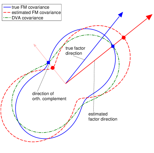
Figure 4: The panel shows the directional variances for an estimated Factor model covariance matrix (red/dashed) and the true Factor model covariance matrix (blue/solid). The blue dots indicate the true variance along the estimated factor direction and the direction of the orthogonal complement. The DVA method (green/dash-dotted) aims at stretching and compressing the estimated covariance peanut such that the variances in these directions correspond to the true ones.

The figure shows in blue/solid and red/dashed the covariances of the true and the estimated factor model, respectively. The arrows indicate the factor directions of the true and estimated factor model and the direction of the orthogonal complement, respectively. Clearly, the factor direction has been misestimated and its strength is overestimated. In the orthogonal direction the variance is underestimated. Our proposed DVA method corrects the systematic error of the directional variance along those directions, without adjusting the directions themselves. This leads to the directional variance adjusted covariance matrix (depicted in green/dash-dotted): In the aforementioned directions, the systematic error is reduced.

One has to keep in mind that the resampling – and with it the estimate of the systematic error of the covariance matrix – is based on the estimated parameters $\cal F$. Therefore, large errors in $\cal F$ adversely affect the DVA covariance estimate.

In order to reduce the impact of the error in $\cal{F}$, it could be advantageous to iterate the DVA procedure. From the DVA covariance matrix, which more closely reflects the true covariance matrix, we could estimate the parameters of a new factor model and restart the DVA procedure, obtaining more precise estimates of correction factors in each iteration. Though a compelling idea, there is no guarantee that iterating the DVA method will give a better solution, converge to a sensible one or even converge at all. In this paper, we therefore concentrate on the non-iterated DVA procedure.

3.4 Simulation Results

Before we present results from daily return data, we will first illustrate the effectiveness of the proposed DVA method in a simulation study. For this, we generate toy data according to the scheme presented in section 3.2, first apply standard Factor Analysis and then use our proposed DVA method to reduce the bias.

The performances of the two estimation methods with respect to the systematic error $S$ (eq. (9)) are contrasted in Figure 5. To the left, it is shown that the DVA method clearly reduces the systematic error of the Factor Analysis model, even for relatively large ratios $T/N$. In the direction of the third factor, which has the lowest SNR, the reduction is most prominent. In the orthogonal complement of the factor subspace, the adjusted spectrum resembles the true variances very well. Nevertheless, there remains a small systematic error, which is due to to using the estimated parameter set in order to infer the directional variance correction factors. The right panel of Figure 5 illustrates that the DVA method does not incur a significant increase in variance of the estimate.

By reducing the systematic error without an increase in variance, the DVA method reduces the average estimation error. To account for different magnitudes of true directional variances, Figure 6 displays the error of the estimator in terms of the mean absolute relative error

$$A^{fa/DVA}_{i}=E\left[\frac{|\sigma^{2\,fa/DVA}_{i}-\sigma^{2\,true}_{i}|}{\sigma^{2\,true}_{i}}\right].$$ (10)

Note that this error is more than halved for the direction of the low SNR-factor and considerably decreased in the orthogonal complement. Here, DVA has the strongest effects on the directions corresponding to the largest and smallest non-zero eigenvalues of $\mathbf{C}^{fa}_{oc}$. For the direction of the smallest eigenvalue, the error is again approximately halved.

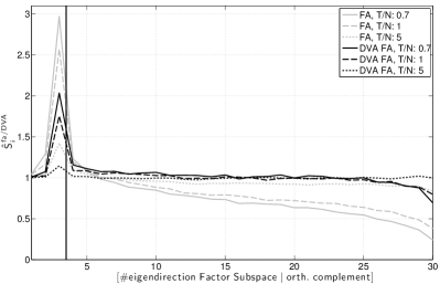
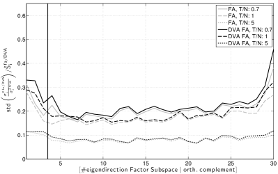
Figure 5: left: comparison of the systematic error for standard Factor Analysis and the DVA Factor Analysis. Right: normalized standard deviation of the error. Simulations for different ratios of sample size to dimensionality ($T/N=0.7$, $1$ and $5$). $N=30$. Correction factors estimated on $K=100$ generated data sets. Mean over 150 simulations.

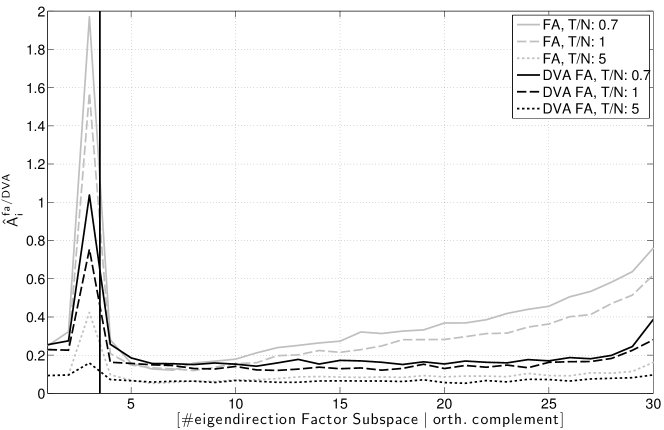
Figure 6: comparison of the mean absolute relative error for standard Factor Analysis and the DVA Factor Analysis for different ratios of sample size to dimensionality ($T/N=0.7$, $1$ and $5$). $N=30$. Correction factors estimated on $K=100$ generated data sets. Mean over 150 simulations.

While the ratio $T/N$ determines most properties of the sample covariance, this is not true for regularized estimators and factor models. For larger values of $T$, at a constant ratio $T/N$, the idiosyncratic variances of Factor Analysis are estimated more precisely, while the estimation of the factors remains difficult. This is shown in Fig. 7, where the dimensionality has been set to 500 and the generative model has seven factors of strength 10, 5, 4, 3, 2.5, 2, 1.5, and 1. One can see that while there is little room for improvement in the orthogonal complement, in the Factor Subspace the performance gain by DVA FA remains on the same level.

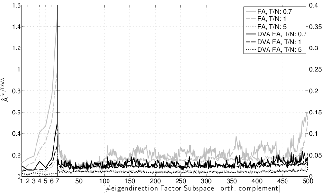
Figure 7: comparison of the mean absolute relative error for standard Factor Analysis and the DVA Factor Analysis for different ratios of sample size to dimensionality ($T/N=0.7$, $1$ and $5$). Note that the y-axis has different scaling for the factor subspace and the orthogonal complement. $N=500$. Correction factors estimated on $K=100$ generated data sets. Mean over 150 simulations.

4 Empirical Results

4.1 Portfolio Simulation

In order to evaluate the proposed methods, we applied the DVA Factor Analysis to financial daily return time series. In the experiments, we estimate covariance matrices of stock returns and use the covariance estimates for portfolio optimization. The realized risks of the portfolios are compared for the different covariance estimates. In particular, we will compare the DVA Factor Analysis to the sample covariance matrix, Resampling Efficiency, the Fama-French Three-Factor model (see, e. g., Fan et al. (2008), Fama and French (1992)), Shrinkage to a one-factor model (Ledoit and Wolf (2003)) and standard Factor Analysis (see section 3.1). For DVA and standard Factor Analysis we use seven factors. Though on the higher dimensional US and EU data sets we could extract more factors and fewer factors would be favorable on the smaller HK data set, we opted for the same intermediate model complexity on all data sets to keep the setting simpler.

4.2 The Data Sets

The data set consists of daily returns of about 1300 US stocks (3.1.2001–2.11.2009), about 600 European stocks (3.1.2001–20.4.2009) and a set of 200 stocks from the Hong Kong stock exchange (3.1.2001–26.9.2008). Removing stocks which do not have data for the whole time horizon covered by the data set, the Hong Kong data set reduces to 100 assets.

4.3 Design of Portfolio Simulations

There are different applications of covariance matrices in portfolio optimization. Covariance matrices are needed for index tracking, hedging and the search for minimum variance portfolios. In the following, we will focus on minimum variance portfolios. The minimum variance portfolio is given by

$$\mathbf{w}^{*}=\mathrm{arg}\!\min_{\mathbf{w}}\;\mathbf{w}^{\top}\hat{\mathbf{C}}\ \mathbf{w},$$ (11)

where $\mathbf{w}$ is the vector of portfolio weights and $\hat{\mathbf{C}}$ is the covariance matrix estimate.

Depending on the particular application, additional constraints are incorporated into the optimization. Commonly applied constraints include:

• $\sum_{i}w_{i}=1$: the sum of all portfolio weights is restricted to one.

• $\mathbf{w}^{\top}\hat{\mathbf{r}}=\mathrm{r}^{*}$: the estimated portfolio return is restricted to $\mathrm{r}^{*}$, $\hat{\mathbf{r}}$ is the vector of expected/predicted asset returns.

• $w_{i}\geq 0$: only positive portfolio weights, no short-selling.

Note that the application of constraints tremendously prunes the set of feasible portfolios and hence diminishes the influence of the covariance estimate (for details, see Jagannathan and Ma (2003)). Consequently, the observed differences between the performances of portfolios obtained from different covariance estimation methods get smaller. Thus, in order to unveil the leverage of the various covariance estimation methods, we opted for not constraining the magnitude of the weights or enforcing their positivity. We only applied the constraint that scales the sum of the portfolio weights to one. In the case of small sample sizes, this approach will tend to overfit the directions of smallest variance and is hence expected to favour the restricted covariance estimators. Therefore, in section 4.5 we also investigate the performances of portfolios obtained from a regularized optimization problem of eq. (11), where the additional regularization enforces diversified portfolios.

In order to evaluate the performance of the different covariance estimator we use the realized (out-of-sample) variance of the estimated portfolios:

$$\sigma^{2}_{real}=\frac{1}{T}\sum_{t=1}^{T}\left[\mathbf{w}_{t-1}^{\top}(\mathbf{r}_{t}-\hat{\mathbf{r}}_{t-1})\right]^{2},$$ (12)

and, of more financial interest, the realized mean absolute deviation

$$\text{MAD}_{real}=\frac{1}{T}\sum_{t=1}^{T}\left|\mathbf{w}_{t-1}^{\top}(\mathbf{r}_{t}-\hat{\mathbf{r}}_{t-1})\right|.$$ (13)

Note, that (12) and (13) are rolling out-of-sample estimates, as $\mathbf{w}_{t-1}$ and $\hat{\mathbf{r}}_{t-1}$ are the portfolio weights and expected returns estimated on the information available until time $t-1$. More precisely, for the estimation of the covariance matrix $\hat{\mathbf{C}}_{t-1}$ and the averaged return $\hat{\mathbf{r}}_{t-1}$ we used a strictly causal window of 150 trading days.

In order to reduce the variance of the performance evaluation and to thoroughly explore the estimated covariance structure, $J=1000$ subsets, each confined to 40 (HK) or 100 (US and EU) assets, are chosen and the optimal (confined) portfolio $\mathbf{w}^{j}_{t}$ is constructed from the given covariance matrix estimate $\hat{C}_{t}^{j}$. The realized variance and realized absolute deviation are then determined based on the average performance across the different confined portfolios, i.e.,

$$\sigma^{2}_{real}=\frac{1}{T}\sum_{t=1}^{T}\left\{\frac{1}{J}\sum_{j=1}^{J}\left[({\mathbf{w}_{t-1}^{j}})^{\top}(\mathbf{r}_{t}-\hat{\mathbf{r}}_{t-1})\right]^{2}\right\},$$

$$\text{MAD}_{real}=\frac{1}{T}\sum_{t=1}^{T}\left\{\frac{1}{J}\sum_{j=1}^{J}\left|({\mathbf{w}_{t-1}^{j}})^{\top}(\mathbf{r}_{t}-\hat{\mathbf{r}}_{t-1})\right|\right\}.$$

4.4 Results and Discussion of Portfolio Simulations

In this section we will provide portfolio simulation results for different covariance estimation approaches, namely the sample covariance matrix, Resampling Efficiency, the Fama-French three-factor model, Shrinkage to a one-factor Model, a Factor Analysis model with seven factors, and a directional variance adjusted Factor Analysis (DVA FA, section 3.2). The results for the different markets are summarized in Table 1.

	US	EU	HK
Sample Cov.	8.56† (156.1†)	5.93† (78.9†)	6.57† (81.2†)
Resampling Eff.	8.83† (165.7†)	6.11† (83.5†)	6.64† (82.7†)
Fama-French	5.65† (73.5†)	3.97† (38.6†)	6.20† (73.4†)
LW Shrinkage	5.56† (69.6†)	4.00† (39.1†)	6.17† (72.9†)
Factor Analysis	5.47† (67.8†)	3.88† (36.5†)	6.17† (73.0†)
DVA FA	5.40 (66.7)	3.84 (36.0)	6.12 (71.7)

Table 1: Mean absolute deviations$\cdot 10^{3}$ (mean squared deviations$\cdot 10^{6}$) of the resulting portfolios for the different covariance estimators and the different markets. ${}^{\dagger}:=$ DVA mean significantly better/worse than this model at the 5% level, tested by a randomization test.

As expected, the sample covariance matrix is not the most suitable tool for portfolio optimization. Across all data sets, the portfolios derived from the different factor based models and Shrinkage clearly outperform the sample covariance matrix based portfolios in terms of realized risk. A direct comparison of these models reveals that the DVA method always significantly outperforms Fama-French, standard Factor Analysis and Shrinkage with respect to realized variance and realized absolute deviation. On our data sets, Resampling Efficiency does not give an advantage over the sample covariance matrix.

4.5 Results and Discussion of Portfolio Simulations – Additional Regularization

Without knowledge of the covariance structure of the assets, the best portfolio allocation would have weights inverse to the variance of the assets and hence be highly diversified. Minimization of eq. (11), on the other hand, gives the optimal portfolio only for the true covariance matrix. Therefore, for a given covariance matrix estimate, it should in principle be possible to additionally reduce the realized risk of a portfolio by increasing its diversification, e.g., by regularization of eq. (11).

Consequently, the aim of the following analysis is twofold. First of all and from a theoretical perspective, we want to investigate if the superior performance of the DVA method can be simply explained away by a higher degree of diversification or if the true covariance structure is indeed better captured. Secondly, with respect to practical considerations, we are interested in the best achievable performance.

In order to analyze these aspects, for each of the covariance matrix estimates $\hat{\mathbf{C}}$ we enforce additional portfolio diversification by including a ridge penalty in the objective function eq. (11), i.e.,

$$\mathbf{w}^{*}(\lambda)=\mathrm{arg}\!\min_{\mathbf{w}}\;\mathbf{w}^{\top}\hat{\mathbf{C}}\ \mathbf{w}+\lambda\mathbf{w}^{\top}\mathbf{\Lambda}\ \mathbf{w}.$$ (14)

In particular, we set the metric $\mathbf{\Lambda}$ to a diagonal matrix which has the single asset variances on its diagonal. This metric implies that each asset gets penalized by its variance and in the limit $\lambda\rightarrow\infty$ we obtain the portfolio of assets weighted by the inverse of their variances.

	US	EU	HK
Sample Cov.	5.45† (67.3†)	3.91† (37.0†)	6.14† (72.8)
Resampling Eff.	5.48† (67.7)	3.93† (37.2)	6.16† (73.4)
Fama-French	5.55† (70.0†)	3.93† (37.7)	6.10 (71.6)
LW Shrinkage	5.39† (65.8)	3.86† (36.3)	6.10 (71.8)
Factor Analysis	5.38† (66.0)	3.82† (35.6)	6.09 (71.7)
DVA FA	5.35 (65.6)	3.81 (35.5)	6.09 (71.3)

Table 2: Mean absolute deviations$\cdot 10^{3}$ (mean squared deviations$\cdot 10^{6}$) of the resulting portfolios for the different regularized covariance estimators for optimal regularization strength and the different markets. ${}^{\dagger}:=$ DVA mean significantly better/worse than this model at the 5% level, tested by a randomization test.

Figure 8 – 10 depict the realized (out-of-sample) variance and MAD (see eq. (12) and eq (13)) of the resulting portfolios as a function of the regularization parameter $\lambda$ for the three different market samples.

In unison, the different models benefit from additional regularization, as can be seen from a reduction of the realized risk of the resulting portfolios (cmp. Tables 1 and 2). Although, this effect is most pronounced for the sample covariance matrix, it merely reaches the performance of the (unregularized) Factor Analysis models. Note that the regularized optimization based on the sample covariance matrix is equivalent to unregularized optimization using a shrinkage covariance estimator, that employs ${\mathbf{C}}^{target}=\mathbf{\Lambda}$ as the shrinkage target (cf. eq. (2)). Again, Resampling Efficiency does not prove to be superior to the sample covariance matrix.

Shrinkage to the one-factor model profits as well from additional Shrinkage to $\mathbf{\Lambda}$. This indicates that the optimization of the expected mean squared error of automatic Shrinkage gives a too small Shrinkage parameter for the optimization of portfolios.

Surprisingly, the Fama-French Three-Factor model does not benefit as much as Shrinkage from the regularization, although the unregularized performance is similar. This implies that the performance gain of the unregularized Fama-French model over the sample covariance matrix is mainly due to a strong imposed prior towards highly diversified portfolios. Compared to the statistical FMs FA, and DVA FA, the performance difference remains on the same level as without additional regularization. This means that the covariance structure is better captured by the statistical FMs than by the Fama-French model. These effects are strongest for the US and EU markets.

The risk of the portfolios obtained from the Factor Analysis model as well as from its DVA version also improve considerably. At the optimal degree of regularization, the DVA FA model significantly outperforms the optimally regularized sample covariance matrix based model for all markets. Regarding eq. (14) as being a shrinkage towards $\mathbf{\Lambda}$, this statement is equivalent to: shrinkage of the DVA Factor Analysis covariance matrix towards $\mathbf{\Lambda}$ yields better portfolios with respect to the achieved portfolio risks than shrinkage of the sample covariance matrix towards $\mathbf{\Lambda}$. The comparison of FA DVA with Fama-French shows a significantly better performance for all markets as well. The performance gain over Shrinkage is, however, only significant for US and EU markets.

At the optimal degree of regularization the difference in performance between the standard Factor Analysis and the DVA Factor Analysis is reduced. In general, this was to be expected as regularization can equivalently be achieved either by adding a penalty term to the objective function or by additionally constraining the feasible set. In this respect, it was shown in Jagannathan and Ma (2003) that the actual influence of the covariance matrix estimate on the minimum variance portfolio diminishes when additionally constraining the set of feasible portfolios. Thus, as a matter of fact, regularization partly compensates for the influence of the systematic error of the Factor Analysis covariance matrix estimate.

Nevertheless, in the US and EU market, the difference in mean MAD remains significant at the 5% level. In Hong Kong the peformance gain of DVA over standard Factor Analysis is, for optimal regularization, not significant.

Comparing the different markets, it turns out that the Hong Kong market shows a slightly different behavior than the American and European. At the Hong Kong market, all methods likewise benefit from additional diversification. One possible explanation is that the HK data set contains quite a few outliers and missing data as opposed to the US and EU data. Thus covariance estimates as well as least square estimates of factor exposures are hampered in general. Hence and in contrast to the other markets, the Fama-French model also clearly profits from the additional regularization, although its overall performance remains inferior to DVA Factor Analysis.

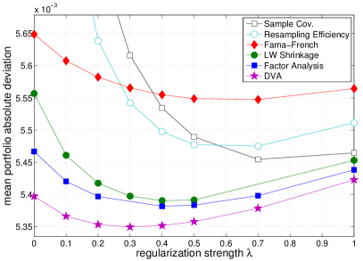
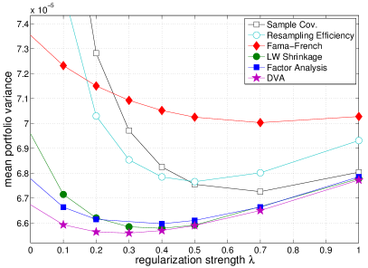
Figure 8: Realized portfolio risk. Left: mean absolute deviation. Right: variance. US market.

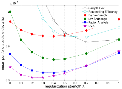
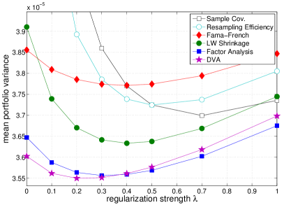
Figure 9: Realized portfolio risk. Left: mean absolute deviation. Right: variance. EU market.

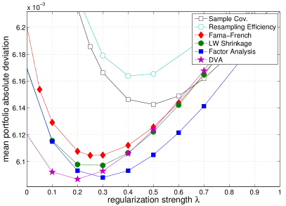
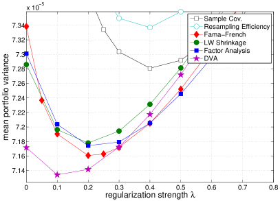
Figure 10: Realized portfolio risk. Left: mean absolute deviation. Right: variance. HK market.

5 Summary

The fundamental issue in portfolio allocation is the accurate and precise estimation of the covariance matrix of asset returns from historical data. Among many challenges, the data is typically high dimensional, noisy, contaminated with outliers and nonstationarity interferes with the use of long estimation windows. Thus, reliable statistical parameter estimation is often impeded. Our work has contributed to alleviate this problem in theoretical and practical aspects: (1) we demonstrated that the data driven statistical Factor Analysis model has a systematic estimation error, which can be alleviated by the proposed algorithmic Directional Variance Adjustment (DVA) framework, (2) a DVA correction of Factor Analysis yields substantial improvements for minimum variance portfolios, and finally (3) extensive simulations of portfolios of EU, US and Hong Kong markets underpinned the usefulness of the DVA approach in terms of significant gains in realized variance and realized mean absolute deviation.

For each covariance estimator, we additionally studied the effect of regularizing the minimum variance portfolios towards a higher degree of diversification. As expected, diversification improved portfolio performance across the different estimators. Our empirical study showed that while regularization slightly decreases the overall advantage gained by DVA, the remaining difference in the minimum stayed significant for the US and EU data sets, here the DVA Factor Analysis method is superior to standard Factor Analysis.

A second interesting finding of the regularization experiments was that the advantage of the Fama-French model over the sample covariance matrix estimator appears rather due to an imposed strong diversification prior than to an improved estimation of the underlying covariance structure. Here, clearly the combination of regularization and statistical FMs like standard FA and in particular DVA FA led to better model performance.

Note, however, that down-weighting/regularizing away the estimated correlations may not always be a valid option. In an application where the covariance structure is of higher importance – e.g. because an index needs to be tracked with a reduced number of assets – increased diversification would clearly be no option.

Therefore, both scenarios, the one with and the one without regularization, yield interesting insight and a clear gain when using DVA FA.

Whilst we have studied and modeled daily returns, the DVA method is of course equally capable of being employed to derive covariances for intraday returns. Intraday covariance matrices are particularly relevant when dealing with portfolios with significant (intraday) churn. Examples of such portfolios include internalization portfolios at most major brokerages, and those used for market making. Using DVA FA, a covariance matrix may be tuned for the typical period a position remains in a portfolio, allowing, potentially, better risk management and asset allocation.

We do not consider serial correlation, as it is common for covariance estimation methods like Shrinkage (see Ledoit and Wolf (2003, 2004)) and statistical Factor Models (see, e.g., Gregory et al. (2010)). Nevertheless, it would be interesting to do further research on an autoregressive Factor Analysis model.

6 Acknowledgements

We are grateful to Gilles Blanchard for his valuable comments. We thank two anonymous reviewers who supplied helpful suggestions which led to substantial improvements of the manuscript.

References

- Abrahamsen and Hansen (2011) Abrahamsen, T. J., Hansen, L. K., Jul. 2011. A cure for variance inflation in high dimensional kernel principal component analysis. J. Mach. Learn. Res. 12, 2027–2044.
- Basilevsky (1994) Basilevsky, A., 1994. Statistical Factor Analysis and Related Methods. John Wiley & Sons, Inc.
- Campbell et al. (2008) Campbell, R. A., Forbes, C. S., Koedjik, K. G., Kofman, P., 2008. Increasing correlations or just fat tails? Journal of Empirical Finance 15, 287–309.
- Comon (1994) Comon, P., 1994. Independent component analysis, a new concept? Signal Process. 36 (3), 287–314.
- Connor (1995) Connor, G., May/June 1995. The three types of factor models: A comparison of their explanatory power. Financial Analysts Journal 51 (3), 42–46.
- Dempster et al. (1977) Dempster, A. P., Laird, N. M., Rubin, D. B., 1977. Maximum likelihood from incomplete data via the EM algorithm. Royal statistical Society B 39, 1–38.
- Edelman and Rao (2005) Edelman, A., Rao, N. R., 2005. Random matrix theory. Acta Numerica 14, 233–297.
- el Karoui (2008) el Karoui, N., 2008. Spectrum estimation for large dimensional covariance matrices using random matrix theory. Annals of Statistics 36 (6), 2757–2790.
- Fama and French (1992) Fama, E. F., French, K. R., June 1992. The cross-section of expected stock returns. Journal of Finance XLVII (2), 427–465.
- Fan et al. (2008) Fan, J., Fan, Y., Lv, J., 2008. High dimensional covariance matrix estimation using a factor model. Journal of Econometrics 147, 186–197.
- Friedman (1989) Friedman, J. H., 1989. Regularized discriminant analysis. J Amer Statist Assoc 84 (405), 165–175.
- Goldfarb and Iyengar (2003) Goldfarb, D., Iyengar, G., 2003. Robust portfolio selection problems. Mathematics of Operations Research 28 (1), 1–38.
- Gregory et al. (2010) Gregory, C., Goldberg, L., Korajcyzk, R., 2010. Portfolio Risk Analysis. Princeton University Press.
- Huber (1981) Huber, P. J., 1981. Robust statistics. Wiley Series in Probability and Mathematical Statistics, New York: Wiley, 1981.
- Hyvärinen and Oja (2000) Hyvärinen, A., Oja, E., 2000. Independent component analysis: algorithms and applications. Neural Netw. 13 (4-5), 411–430.
- Jagannathan and Ma (2003) Jagannathan, R., Ma, T., August 2003. Risk reduction in large portfolios: Why imposing the wrong constraints helps. Journal of Finance LVIII (4), 1651–1683.
- Jolliffe (1986) Jolliffe, I. T., 1986. Principal component analysis. Springer Series in Statistics, Berlin: Springer, 1986.
- Jöreskog (1967) Jöreskog, K. G., 1967. Some contributions to maximum likelihood factor analysis. Psychometrika 32, 443–482.
- Kjems et al. (2001) Kjems, U., Hansen, L. K., Strother, S. C., 2001. Generalizable singular value decomposition for ill-posed datasets. Advances in Neural Information Processing Systems 13, 549–555.
- Laloux et al. (2000) Laloux, L., Cizeau, P., Potters, M., Bouchaud, J.-P., 2000. Random matrix theory and financial correlations. International Journal of Theoretical and Applied Finance 3 (3), 391–397.
- Ledoit and Wolf (2003) Ledoit, O., Wolf, M., 2003. Improved estimation of the covariance matrix of stock returns with an application to portfolio selection. Journal of Empirical Finance 10, 603–621.
- Ledoit and Wolf (2004) Ledoit, O., Wolf, M., 2004. A well-conditioned estimator for large-dimensional covariance matrices. J Multivar Anal 88 (2), 365–411.
- Longin (2005) Longin, F., 2005. The choice of the distribution of asset returns: How extreme value theory can help? Journal of Banking and Finance 29, 1017–1035.
- Loretan and Phillips (1994) Loretan, M., Phillips, P. C., 1994. Testing the covariance stationarity of heavy-tailed time series. Journal of Empirical Finance 1, 211–248.
- Markowitz (1952) Markowitz, H., March 1952. Portfolio selection. Journal of Finance VII (1), 77–91.
- Marčenko and Pastur (1967) Marčenko, V. A., Pastur, L. A., 1967. Distribution of eigenvalues for some sets of random matrices. Mathematics of the USSR-Sbornik 1 (4), 457.
- McLachlan et al. (2007) McLachlan, G., Bean, R., Jones, L. B.-T., 2007. Extension of the mixture of factor analyzers model to incorporate the multivariate t-distribution. Computational Statistics and Data Analysis 51 (11), 5327 – 5338.
- Michaud (1998) Michaud, R. O., Jun. 1998. Efficient Asset Management: A Practical Guide to Stock Portfolio Optimization and Asset Allocation. Oxford University Press, USA.
- Miller (2006) Miller, G., 2006. Needles, haystacks and hidden factors. Journal of Portfolio Management 32 (2), 25–32.
- Pagan and Schwert (1990) Pagan, A. R., Schwert, G. W., 1990. Testing for covariance stationarity in stock market data. Economics Letters 33, 165–170.
- Roll and Ross (1980) Roll, R., Ross, S. A., December 1980. An empirical investigation of the arbitrage pricing theory. Journal of Finance XXXV (5), 1073–1103.
- Rosenow et al. (2002) Rosenow, B., Plerou, V., Gopikrishnan, P., Stanley, H. E., 2002. Portfolio optimization and the random magnet problem. Europhys. Letters, 500–506.
- Roweis and Ghahramani (1999) Roweis, S., Ghahramani, Z., 1999. A unifying review of linear gaussian models. Neural Computation 11 (2).
- Rubin and Thayer (1982) Rubin, D., Thayer, D., Mar. 1982. EM algorithms for ML factor analysis. Psychometrika 47 (1), 69–76.
- Schäfer and Strimmer (2005) Schäfer, J., Strimmer, K., 2005. A shrinkage approach to large-scale covariance matrix estimation and implications for functional genomics. Statistical Applications in Genetics and Molecular Biology 4 (1).
- Scherer (2004) Scherer, B., 2004. Resampled efficiency and portfolio choice. Financial Markets and Portfolio Management 18 (4), 382–398.
- Shanken (1992) Shanken, J., 1992. On the estimation of beta pricing models. Review of Financial Studies 5, 1–34.
- Stein (1956) Stein, C., 1956. Inadmissibility of the usual estimator for the mean of a multivariate normal distribution. In: Proc. 3rd Berkeley Sympos. Math. Statist. Probability. Vol. 1. pp. 197–206.
- Tipping and Bishop (1999) Tipping, M. E., Bishop, C. M., 1999. Probabilistic Principal Component Analysis. Journal of the Royal Statistical Society, Series B 61, 611–622.
- Tulino and Verdú (2004) Tulino, A. M., Verdú, S., June 2004. Random matrix theory and wireless communications. Commun. Inf. Theory 1, 1–182.
- Zhao et al. (2008) Zhao, J.-H., Yu, P. L. H., Jiang, Q., 2008. ML estimation for factor analysis: EM or non-EM? Statistics and Computing, 109–123.