A Remark on the Geometry of Uniformly Rotating Stars

Abstract.

In this paper we classify the free boundary associated to equilibrium configurations of compressible, self-gravitating fluid masses, rotating with constant angular velocity. The equilibrium configurations are all critical points of an associated functional and not necessarily minimizers. Our methods also apply to alternative models in the literature where the angular momentum per unit mass is prescribed. The typical physical model our results apply to is that of uniformly rotating white dwarf stars.

1. Introduction

In this paper we study the free boundary associated to rotating star models of white dwarf stars with prescribed constant angular velocity. Thus we are considering figures of equilibrium for compressible, self-gravitating fluid masses.

There has been a tremendous amount of work on incompressible, self-gravitating fluid masses rotating with prescribed constant angular velocity since the primary investigations by Newton. Various mathematicians like MacLaurin, Jacobi, Dirichlet, Riemann, Poincaré, H. Cartan and Chandrasekhar made significant contributions to the field, studying bifurcation sequences and analyzing the stability of various equilibrium shapes. A historical account and details of these investigations may be found in Chandrasekhar’s treatise [10] and Tassoul’s book [17].

In the compressible case for the model with prescribed constant angular velocity $\omega>0$ (cf. [14]), we consider the functional

(1.1) $$J(\rho)=\int_{\mathbb{R}^{3}}A(\rho)\>d\xi-{1\over 2}\int_{\mathbb{R}^{3}}\omega^{2}r^{2}\rho\>d\xi-\int_{\mathbb{R}^{3}}\rho B\rho\>d\xi,$$

where $\xi=(\xi_{1},\xi_{2},\xi_{3}),r=\sqrt{\xi_{1}^{2}+\xi_{2}^{2}},\rho\geq 0,\rho\in L^{1}(\mathbb{R}^{3})\cap L^{\infty}(\mathbb{R}^{3})$ and

$$(B\rho)(\xi)=\int_{\mathbb{R}^{3}}\frac{\rho(\eta)}{|\xi-\eta|}\>d\eta.$$

Moreover we impose the constraint

(1.2) $$\int_{\mathbb{R}^{3}}\rho=1.$$

As $\rho(\xi)$ represents the density of the stellar material, (1.2) means that the mass of the star is prescribed. Later in our paper we will assume in addition that the density $\rho(\xi)$ is axisymmetric, i.e.

$$\rho(\xi)=\rho(r,z)\textrm{ where }z(\xi)=\xi_{3}.$$

This assumption means that the star is rotating about the $\xi_{3}$-axis. The function $A(\rho)$ is the pressure and thus represents the equation of state of the stellar material. We assume that $A(\rho)\in C^{1}([0,+\infty))$ with $A$ strictly convex so that $A^{\prime}(\rho)$ is invertible. Further conditions on $A(\rho)$ will be stipulated below. The first term in (1.1) represents then the internal energy of the star, the second term the rotational kinetic energy and the last term the gravitational potential energy.

In [14] the existence of minimizers of $J$ under the constraint (1.2) has been obtained. [13] contains further results for this model of prescribed angular velocity. In [11] support estimates for critical points of (1.1) under the constraint (1.2) have been shown. In particular, [11, Theorem 1] states that for $\omega\geq\omega_{0}>0$, the support of $\rho$ is contained in a ball $B_{\sigma}(0,0,\xi_{3})$ for some $\xi_{3}$, where $\sigma=\sigma(\omega_{0})$. It follows that

$$0\leq B\rho\leq C\textrm{ in }\mathbb{R}^{3}.$$

Furthermore, [11, Theorem 2] shows that the number of connected components of the set $\{\rho>0\}$ is finite for any critical point $\rho$.

Critical points of $J$ with the constraint (1.2) are according to [11, (0.6)] characterized by the problem

(1.3) $$\rho\textrm{ is continuous and nonnegative and }A^{\prime}(\rho)-{1\over 2}\omega^{2}r^{2}-B\rho=\lambda(\omega)\textrm{ in }\{\rho>0\},$$

where $\lambda(\omega)$ is a Lagrange multiplier arising from the constraint (1.2). The focus in this paper is to study the free boundary $\partial\{\rho>0\}$ arising from (1.3).

There is another model of rotating stars which has been studied in the literature, where the angular momentum per unit mass is prescribed. Existence of minimizers for this alternative model has been obtained in [5], and the study of critical points has been carried out in [15]. Caffarelli-Friedman investigated in [7] the free boundary of minimizers for this alternative model. As Caffarelli-Friedman deal with minimizers, they are able to apply rearrangement methods to their functional to obtain solutions that are increasing in one direction which simplifies the analysis as well as the result. Unfortunately this technique does not work for critical points in either model and creates a difficulty for our analysis. Let us remark that the proofs presented in this paper for critical points of $J$ with the constraint (1.2) work equally well for the study of the free boundary of critical points in the model in [7].

The principal difficulty we encounter in our classification of singularities of the free boundary is that the nonlinearity is not an increasing function of the solution, so that various methods stemming from the well-known obstacle problem do not apply. Neither does the monotonicity formula derived in [1]. Let us also mention that our problem cannot be transformed into the type of problems studied in [8], so we cannot use those results either. Another difficulty is that our equation is inhomogeneous. In particular, the leading order term on the right-hand side is not of the form $f(u)$. This —together with a higher order degeneracy— distinguishes the present problem also from the recently researched “unstable obstacle problem” (see [16], [2], [4] and [3]).

Last, let us point out that —due to the fact that the free boundary $\partial\{\rho>0\}$ does not necessarily coincide completely with the free boundary of the PDE problem obtained by transformation— we obtain in our classification of singularities several cases later called “pseudo cases.” We suggest that in the case of minimizers, rearrangement techniques similar to those used in [7] may be used to show that solutions are decreasing in a certain direction, thus ruling out the pseudo cases.

Setting $u={1\over 2}\omega^{2}r^{2}+B\rho+\lambda(\omega)$, we obtain in the set $\overline{\{\rho>0\}}$ that $u=A^{\prime}(\rho)=\Phi^{-1}(\rho),$ where $\Phi:[0,+\infty)\to\mathbb{R}$ is an increasing function satisfying according to the asymptotics

$$A(\rho)=c_{1}\rho^{5\over 3}+o(\rho^{5\over 3})\textrm{ as }\rho\to 0,A(\rho)=c_{2}\rho^{4\over 3}+o(\rho^{4\over 3})\textrm{ as }\rho\to+\infty$$

(where $c_{1},c_{2}$ are positive constants) from Chandrasekhar’s book [9, Chapter 10] and [11, (0.2)] the asymptotic relations

(1.4) $$A^{\prime}(\rho)={5\over 3}c_{1}\rho^{2\over 3}+o(\rho^{2\over 3})\textrm{ as }\rho\to 0, A^{\prime}(\rho)={4\over 3}c_{2}\rho^{1\over 3}+o(\rho^{1\over 3})\textrm{ as }\rho\to 0,$$

(1.5) $$\lim_{z\to 0+}z^{-3/2}\Phi( z)=c>0.$$

It follows (cf. [11, (3.3)]) that

$$\Delta u=3\omega^{2}-4\pi\rho=3\omega^{2}-4\pi\Phi(u)\textrm{ in }\{\rho>0\}$$

and

$$\Delta u=3\omega^{2}\textrm{ in }\{\rho=0\}.$$

Note that as $u=A^{\prime}(\rho)=\Phi^{-1}(\rho)$ is only valid in the set $\overline{\{\rho>0\}}$, we obtain $\{\rho>0\}\subset\{u>0\}$ but not necessarily the opposite inclusion. It is however true that $\partial\{\rho>0\}=\partial\{u>0\}$ and that if $\rho(x^{0})>0$ then the connected component of $\{\rho>0\}$ containing $x^{0}$ coincides with the connected component of $\{u>0\}$ containing $x^{0}$.

Normalizing the equation as well as $\Phi$ we obtain the free boundary problem

(1.6) $$\Delta u=1-\Phi(u)\chi_{\Omega}\textrm{ with an open set }\Omega\textrm{ satisfying }\chi_{\Omega}\leq\chi_{\{u>0\}};$$

the equation is to be understood in the sense of distributions.

Theorem A.

For each solution $u$ of problem (1.6) the following holds: Apart from the singular set $S=\{u=0\}\cap\{\nabla u=0\}$ the level set $\{u=0\}$ and the boundary $\partial\Omega$ are locally $C^{2,\alpha}$-curves. The singular set contains in each bounded subset of $\mathbb{R}^{2}$ at most finitely many singular points $x^{0}$ with the following possible asymptotics (after rotation of the coordinate system):

1. $u(x^{0}+tx)/t^{2}\to{1\over 2}x_{1}^{2}$ as $t\to 0$, and $\{u>0\}$ and $\Omega$ satisfy the asymptotics demonstrated in Figure 1.

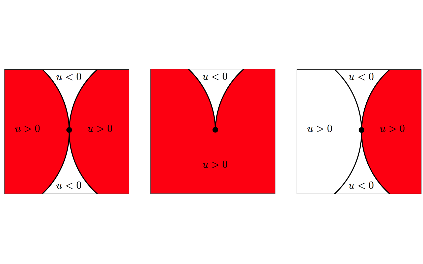
Figure 1. Cusps (with the set $\Omega$ painted red)

2. There is $\lambda\in(-\infty,0)\cup(1,+\infty)$ such that $u(x^{0}+tx)/t^{2}\to{1\over 2}\left(\lambda x_{1}^{2}+(1-\lambda)x_{2}^{2}\right)$ as $t\to 0$. We may assume that $\lambda>1$ in which case $\{u>0\}$ and $\Omega$ satisfy the asymptotics demonstrated in Figure 2.

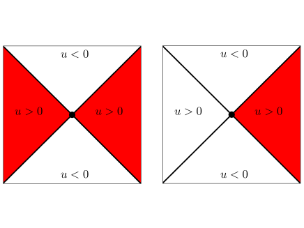
Figure 2. Wedges (with the set $\Omega$ painted red)

3. There is $\lambda\in(0,1)$ such that $u(x^{0}+tx)/t^{2}\to{1\over 2}\left(\lambda x_{1}^{2}+(1-\lambda)x_{2}^{2}\right)$ as $t\to 0$. The complement of $\{u>0\}$ and that of $\Omega$ is the single point $x^{0}$.

2. Proof of the Main Result

Let $u$ be a solution of (1.6). By $L^{p}$- and $C^{\alpha}$-estimates $u\in W^{2,p}_{\rm loc}(\mathbb{R}^{3})\cap C^{1,\alpha}_{\rm loc}(\mathbb{R}^{3})$ for each $p\in(1,+\infty)$ and $\alpha\in(0,1)$. Differentiating $u$ we obtain

(2.1) $$\Delta\partial_{k}u=-\Phi^{\prime}(u)\chi_{\Omega}\partial_{k}u\in L^{\infty}_{\rm loc}(\mathbb{R}^{3})$$

in the sense of distributions. Consequently $u\in W^{3,p}_{\rm loc}(\mathbb{R}^{3})\cap C^{2,\alpha}_{\rm loc}(\mathbb{R}^{3})$ for each $p\in(1,+\infty)$ and $\alpha\in(0,1)$. From (1.6) we infer now that the Hessian of $u$ satisfies

$$|D^{2}u|\geq c(n)>0\textrm{ on }\{u=0\}.$$

As $\{u=0\}\cap\{\nabla u\neq 0\}$ is by the implicit function theorem locally a $C^{2,\alpha}$-surface —the regularity of the surface can be improved to real analyticity by the methods in [7]—, we will focus on the singular set $S=\{u=0\}\cap\{\nabla u=0\}$. From now on we will assume that $u$ is axisymmetric, that is $u=u(r,x_{3})$ and confine ourselves thus to a two-dimensional analysis.

At each $x^{0}\in S$ we may rotate axes such that

$$D^{2}u(x^{0})=\begin{pmatrix}\lambda&0\\ 0&1-\lambda\end{pmatrix}\textrm{ for some }\lambda\in\mathbb{R}.$$

Case 1: If $0<\lambda<1$, then $\Omega^{c}$ consists in a sufficiently small ball $B_{\delta}(x^{0})$ of only the point $x^{0}$ which is in this case a local minimum point of $u$.
Case 2: If $\lambda>1$ or $\lambda<0$, $\{u=0\}$ consists of two $C^{1}$-curves intersecting at a nonzero angle at $x^{0}$ (cf. Figure 3 and Figure 4): we may assume that $x^{0}=0$ and that $\lambda>1$. As in this case for sufficiently small $\delta$, $\partial_{x_{1}}u>0$ in $B_{r}\cap\{x_{1}>\delta\}$ and $\partial_{x_{1}}u<0$ in $B_{r}\cap\{x_{1}<-\delta\}$, we may rescale and obtain that $\{u=0\}\setminus\{0\}$ consists of four $C^{1,\alpha}$-graphs. The fact that

$$u(tx)/t^{2}\to{1\over 2}\left(\lambda x_{1}^{2}+(1-\lambda)x_{2}^{2}\right)\textrm{ as }t\to 0$$

implies now that the graphs have tangents as $x\to 0$ and that we may combine them to two $C^{1}$-curves intersecting at a nonzero angle at $0$.

Figure 3. Double Wedge (with the set $\Omega$ painted red)

Figure 4. Pseudo Wedge (with the set $\Omega$ painted red)

Case 3: If $\lambda=1$ or $\lambda=0$, then $\{u=0\}$ consists either of two $C^{1}$-curves ending in a cusp at $x^{0}$ (cf. Figure 6) or intersecting in a double cusp at $x^{0}$ (cf. Figure 7): we may assume $x^{0}=0$ and $\lambda=1$, implying that $u(tx)/t^{2}\to{1\over 2}x_{1}^{2}$ as $t\to 0$. From (2.1) with $k=2$ we obtain that

$$\Delta\partial_{2}u=c(x)\partial_{2}u$$

with Hölder continuous coefficients $c(x)$. Applying [6, Lemma 3.1] repetitively for $\beta=3/2,7/2,11/2,15/2,\dots$ we infer that either

$$\partial_{2}u=p+\Gamma$$

where $p$ is a nontrivial harmonic polynomial of degree $[\beta]+2$ with leading term of order $\geq 2$ (by the fact that $u(tx)/t^{2}\to{1\over 2}x_{1}^{2}$ as $t\to 0$) and

$$|\Gamma(x)|\leq C_{1}|x|^{\beta+2},$$

or $\partial_{2}u$ vanishes of infinite order at $0$, that is

$$|\partial_{2}u(x)|\leq C_{k}|x|^{k}\textrm{ in }B_{r_{k}}(0)$$

for every $k\in\mathbb{N}$. In the latter case we obtain by repetitive application of a well-known strong unique continuation property (see [12, Remark 6.7] for a very general result), that

$$\partial_{2}u\equiv 0\textrm{ in each connected component of }\{u\neq 0\}\textrm{ touching the origin,}$$

implying by our information on the blow-up limit that

$$u\equiv{1\over 2}x_{1}^{2}+f(x_{1})\textrm{ in each connected component of }\{u\neq 0\}\textrm{ touching the origin,}$$

where $f(z)\to 0$ as $z\to 0$. But this contradicts the constraint $\int_{\mathbb{R}^{3}}\rho=1$, thus proving that infinite order vanishing is not possible.

Let us return to the former case

$$\partial_{2}u=q+O(|x|^{k+{1\over 2}})$$

where $q$ is a nontrivial homogeneous harmonic polynomial of degree $k\geq 2$. It is important to note that —by the fact that $q$ is harmonic— if $q((0,1))=0$ then $\partial_{x_{1}}q((0,1))\neq 0$. Similarly, if $q((0,-1))=0$ then $\partial_{x_{1}}q((0,-1))\neq 0$.

It follows that

$$u={1\over 2}x_{1}^{2}+\int_{0}^{x_{2}}q(x_{1},s)\>ds+O(|x|^{k+{3\over 2}}).$$

In this case $\{u<0\}$ is in a neighborhood of $0$ a one-sided or two-sided cusp (depending on the signs of $q((0,1))$ and $q((0,-1))$); see Figure 6 and Figure 7. In the special case that $q((0,1))=0$ or $q((0,-1))=0$, we obtain $\partial_{x_{1}}q((0,1))\neq 0$ or $\partial_{x_{1}}q((0,-1))\neq 0$, respectively, in which case we obtain a non-symmetric cusp (even asymptotically) with respect to the $x_{1}$-axis on the side of $(0,1)$ or $(0,-1)$, respectively.

Figure 5. Pseudo Cusp (with the set $\Omega$ painted red)

Figure 6. Double Cusp (with the set $\Omega$ painted red)

Figure 7. Cusp (with the set $\Omega$ painted red)

References

- [1] Hans Wilhelm Alt, Luis A. Caffarelli, and Avner Friedman. Variational problems with two phases and their free boundaries. Trans. Amer. Math. Soc., 282(2):431–461, 1984.
- [2] J. Andersson and G. S. Weiss. Cross-shaped and degenerate singularities in an unstable elliptic free boundary problem. J. Differential Equations, 228(2):633–640, 2006.
- [3] John Andersson, Henrik Shahgholian, and Georg S. Weiss. On the singularities of a free boundary through fourier expansion. Invent. Math.
- [4] John Andersson, Henrik Shahgholian, and Georg S. Weiss. Uniform regularity close to cross singularities in an unstable free boundary problem. Comm. Math. Phys., 296(1):251–270, 2010.
- [5] J. F. G. Auchmuty and Richard Beals. Variational solutions of some nonlinear free boundary problems. Arch. Rational Mech. Anal., 43:255–271, 1971.
- [6] Luis A. Caffarelli and Avner Friedman. The free boundary in the Thomas-Fermi atomic model. J. Differential Equations, 32(3):335–356, 1979.
- [7] Luis A. Caffarelli and Avner Friedman. The shape of axisymmetric rotating fluid. J. Funct. Anal., 35(1):109–142, 1980.
- [8] Luis A. Caffarelli and Avner Friedman. Partial regularity of the zero-set of solutions of linear and superlinear elliptic equations. J. Differential Equations, 60(3):420–433, 1985.
- [9] S. Chandrasekhar. An introduction to the study of stellar structure. Dover Publications Inc., New York, N. Y., 1957.
- [10] S. Chandrasekhar. Ellipsoidal figures of equilibrium. Dover Publications Inc., New York, N. Y., 1992.
- [11] Sagun Chanillo and Yan Yan Li. On diameters of uniformly rotating stars. Comm. Math. Phys., 166(2):417–430, 1994.
- [12] David Jerison and Carlos E. Kenig. Unique continuation and absence of positive eigenvalues for Schrödinger operators. Ann. of Math. (2), 121(3):463–494, 1985. With an appendix by E. M. Stein.
- [13] Haigang Li and Jiguang Bao. Existence of rotating stars with prescribed angular velocity law. Houston J. Math., 37(1):297–309, 2011.
- [14] Yan Yan Li. On uniformly rotating stars. Arch. Rational Mech. Anal., 115(4):367–393, 1991.
- [15] Tao Luo and Joel Smoller. Rotating fluids with self-gravitation in bounded domains. Arch. Ration. Mech. Anal., 173(3):345–377, 2004.
- [16] R. Monneau and G. S. Weiss. An unstable elliptic free boundary problem arising in solid combustion. Duke Math. J., 136(2):321–341, 2007.
- [17] J.L. Tassoul. Theory of rotating stars. Princeton Univ. Press, New Jersey, 1978.