Finite temperature phase diagram of spin-$1/2$ bosons in two-dimensional optical lattice

Abstract

We study a two-species bosonic Hubbard model on a two-dimensional square lattice by means of quantum Monte Carlo simulations and focus on finite temperature effects. We show in two different cases, ferro- and antiferromagnetic spin-spin interactions, that the phase diagram is composed of a superfluid phase and an unordered phase that can be separated into weakly compressible Mott insulators regions and compressible Bose liquid regions. The superfluid-liquid transitions are of the Berezinsky-Kosterlitz-Thouless type whereas the insulator-liquid passages are crossovers. We analyse the pseudo-spin correlations that are present in the different phases, focusing particularly on the existence of a polarization in this system.

I Introduction

The study of strongly interacting quantum models by direct realization of an experimental system reproducing the model properties, an idea proposed by Feynman feynman82 , was realized in the past ten years with the production of Bose-Einstein condensates (BEC) and their use as “quantum simulators” bloch08 . In particular, BEC in conjunction with optical lattices are used to produce systems reproducing the physics of well known quantum statistical discrete models such as fermionic or bosonic Hubbard models.

Used to study simple models of bosons bloch02 or fermions kett09 at low temperature, the flexibility offered by these systems extends the range of interesting models to more exotic ones which can be treated both experimentally and theoretically. Examples include systems with long range interactions pfau05 , fermions with imbalanced populations kett06 , mixtures of different kinds of particles kett07 and spin-1 bosons with spin-independent and spin-dependent interactions which allow interplay between superfluidity and magnetism stamper ; stamper2 ; ggb09 . Furthermore, it is possible to study systems of bosons with two effective internal degrees of freedom on an optical lattice, the so-called “spin-$1/2$ bosons”. Such a system, with spin-dependent interactions, could be produced by applying a periodic optical lattice on a bosonic system with two triply degenerate internal energy levels. The optical potential applied would localise the atoms at the nodes of a regular network, but would also couple the internal states by $\Lambda$ or V virtual processes, thus leaving only two internal low energy degenerated states denoted $0$ and $\Lambda$ and realizing an effective spin-$1/2$ model krutitsky04 ; larson . The presence of the spin-dependent interaction introduces a term in the Hamiltonian which permits the conversion of two particles of one type into the other type and renders numerical simulations more difficult. This model is related, but not identical, to other models including p-band superfluid models wu06a ; wu06b ; wu09 and the bosonic Kondo model fossfeig . Understanding the phase diagram and properties of the simpler spin-$1/2$ bosonic system takes us a step toward understanding the more elaborate, and more difficult to simulate, models.

The spin-$1/2$ model has been extensively studied with mean-field theory (MFT) at zero or finite temperatures and, in previous work, we explored its zero temperature behavior with quantum Monte Carlo (QMC) simulations in one deforges10 and two deforges11 dimensions for on-site repulsive interactions. At zero temperature, the phase diagrams obtained in one and two dimensions, with MFT or QMC, are similar. Generally speaking, at zero temperature, the system can adopt two different kinds of phases: insulating Mott phases that appear for integer density, $\rho$, and for large enough repulsion between particles and superfluid phases (SF) otherwise. The detailed nature of these phases depends on the interactions between the different kinds of particles. In the case where the repulsion between identical particles is smaller than between different particles ($U_{2}>0$ in our previous work deforges11 and in the following) the superfluid is found to be polarized, that is, an imbalance develops in the populations of the two kinds of particles and one of the species becomes dominant. The $\rho=1$ Mott phase is also polarized whereas the $\rho=2$ phase is not (we did not study higher densities with QMC). In the opposite case, $U_{2}<0$, all the phases are unpolarized. Noteworthy is the presence of coherent exchange movements kuklov03 , where two particles of different types exchange their position in the $\rho=1$ Mott phase in both cases, as well as in the $\rho=2$ Mott phase for $U_{2}<0$. Finally, in one dimension, all zero temperature phase transitions were found to be continuous whereas in two dimensions and when $U_{2}>0$ is small enough, the $\rho=2$ Mott-superfluid transition was predicted by MFT to be first order near the tip of the Mott lobe and continuous otherwise, whereas for larger $U_{2}$ the transition was predicted to be always continuous. This was confirmed by QMC simulations deforges11 . Related spin-1 models were studied using MFT Pai08 ; kimura or QMC in one dimension ggb09 and a similar spin 1/2 bosons model was also recently studied takayoshi10 .

In this paper, we will study the spin-$1/2$ model at finite temperature in two dimensions and compare with MFT predictions. The results for finite system sizes and temperatures are relevant to experimental efforts to study this system. In Section II, we will introduce the model and the MFT and QMC techniques used to study it. Section III and IV will be devoted to the presentation of the results obtained for the $U_{2}>0$ and $U_{2}<0$ cases, respectively. We will summarize these results and give some final remarks in Section IV.

II Spin-1/2 Model

The model we will study is the same we previously studied in the low temperature limit in one deforges10 and two dimensions deforges11 and previously introduced in krutitsky04 . It is an extended Hubbard model governed by the Hamiltonian

$$\mathcal{H}=-t\sum_{\sigma,\langle{\bf r,r^{\prime}}\rangle}\left(a^{\dagger}_{\sigma{\bf r}}a_{\sigma{\bf r^{\prime}}}+a^{\dagger}_{\sigma{\bf r^{\prime}}}a_{\sigma{\bf r}}\right)-\mu\sum_{\sigma,{\bf r}}\hat{n}_{\sigma{\bf r}}$$ (1)

$$+\,\frac{U_{0}}{2}\sum_{\sigma,{\bf r}}\hat{n}_{\sigma{\bf r}}(\hat{n}_{\sigma{\bf r}}-1)+(U_{0}+U_{2})\sum_{\bf r}\hat{n}_{0{\bf r}}\hat{n}_{\Lambda{\bf r}}$$ (2)

$$+\frac{U_{2}}{2}\sum_{\bf r}\left(a_{0{\bf r}}^{\dagger}a_{0{\bf r}}^{\dagger}a_{\Lambda{\bf r}}a_{\Lambda{\bf r}}+a_{\Lambda{\bf r}}^{\dagger}a_{\Lambda{\bf r}}^{\dagger}a_{0{\bf r}}a_{0{\bf r}}\right),$$ (3)

where operator $a_{\sigma{\bf r}}$ ($a^{\dagger}_{\sigma{\bf r}}$) destroys (creates) a boson of type $\sigma=0,\Lambda$ on site $\bf r$ of a two-dimensional square lattice of size $L\times L$. The operators $\hat{n}_{\sigma{\bf r}}$ measures the number of particles of type $\sigma$ on site $\bf r$. The densities of particles of type 0 and $\Lambda$ are called $\rho_{0}$ and $\rho_{\Lambda}$ while the total density is called $\rho=\rho_{0}+\rho_{\Lambda}$.

The first term (1) of the Hamiltonian is the kinetic term that lets particles hop from site $\bf r$ to its nearest neighbours $\bf r^{\prime}$. The associated hopping energy $t=1$ sets the energy scale. A chemical potential $\mu$ is added if one works in the grand canonical ensemble. The second term (2) describes on-site repulsion between identical particles with a strength $U_{0}$ or between different particles with a strength $U_{0}+U_{2}$. We will study both the positive and negative $U_{2}$ cases but will keep only repulsive interactions, that is $|U_{2}|<U_{0}$, and a fixed moderate value of $|U_{2}|/U_{0}=0.1$. The last term (3) provides a possibility to change the “spins” of the particles: When two identical particles are on the same site, they can be transformed into two particles of the other type. It was demonstrated in krutitsky04 that the matrix element associated with this conversion is $U_{2}/2$. We are using a different sign for the term (3) compared to the articles where the model was originally introduced krutitsky04 but we have shown in a previous work deforges10 that this sign can indeed be chosen freely due to a symmetry of the model.

II.1 Mean Field Theory

The only term that couples different sites in the Hamiltonian is the hopping term (1). Introducing the field $\psi_{\sigma}=\langle a^{\dagger}_{\sigma{\bf r^{\prime}}}\rangle=\langle a_{\sigma{\bf r^{\prime}}}\rangle$, we replace the creation/destruction operators on site ${\bf r^{\prime}}$ by their mean values $\psi_{\sigma}$, following the approach used in krutitsky04 . The Hamiltonian on site $\bf r$ is then decoupled from neighboring sites and can be easily diagonalized numerically in a finite basis. The optimal value of the fields $\psi_{\sigma}$ are then chosen by minimizing the grand canonical potential $\mathcal{G}=-kT\ln{\cal Q}$ with respect to $\psi_{\sigma}$ where ${\cal Q}$ is the grand canonical partition function. The system is in a superfluid phase when $\psi_{\sigma}$ is nonzero, with superfluid density $\rho_{s}=|\psi_{0}|^{2}+|\psi_{\Lambda}|^{2}$, and is otherwise in an unordered phase where two cases can be distinguished: an almost incompressible case, i.e. a Mott insulator, and a compressible case, i.e. a liquid.

In these two cases there is no broken symmetry and they cannot be distinguished by symmetry considerations. If there is a first order transition between the MI and the liquid, characterized by discontinuities in the density or other thermodynamic functions, the MI and the liquid would be two distinct phases. If, however, there is no discontinuity in the evolution from the MI to the liquid then they are only two limiting cases of the same unordered phase and there is only a smooth crossover between the MI and the liquid regions of the phase diagram. We shall see that, indeed, there is a crossover in the system we are considering here.

One can distinguish between almost-incompressible and liquid regions by calculating the local density variance which is a measure of the local compressibility, ${\tilde{\kappa}}=\beta\left(\langle n_{\bf r}^{2}\rangle-\langle n_{\bf r}\rangle^{2}\right)$ where $n_{\bf r}$ is the total number of particles on site $\bf r$. ${\tilde{\kappa}}$ is close to zero in the Mott phase and much larger in the liquid phase.

While this MFT was shown to reproduce qualitatively the phase diagram at zero temperature deforges11 , it is rather limited at finite temperature. Indeed, whenever the $\psi_{\sigma}$ are zero the hopping parameter $t$ no longer plays a rôle in the MFT. Then, while the MFT can distinguish between SF and unordered phases, it does not correctly distinguish Mott Insulator (MI) regions from normal Bose liquids ones, as the crossover boundary between those regions will not depend on $t$ and will be the same as in the $t=0$ case.

II.2 Quantum Monte Carlo simulations

To simulate this system, we used the stochastic Green function algorithm (SGF) SGF , an exact Quantum Monte Carlo (QMC) technique that allows canonical or grand canonical simulations of the system at finite temperatures as well as measurements of many-particle Green functions. In particular, this algorithm can simulate efficiently the spin-flip term in the Hamiltonian. We studied sizes up to $L=14$. The density $\rho$ is conserved in canonical simulations, but individual densities $\rho_{0}$ and $\rho_{\Lambda}$ fluctuate due to the conversion term Eq. (3). The superfluid density is given by fluctuations of the total winding number, $(W_{0}+W_{\Lambda})$, of the world lines of the particles roy

$$\rho_{s}=\frac{\langle(W_{0}+W_{\Lambda})^{2}\rangle}{4t\beta}.$$ (4)

The superfluid density cannot be measured separately for $0$ and $\Lambda$ particles due to the conversion term roscilde10 . It, therefore depends on the total density not on the separate densities of the two species. We also calculate the one particle Green functions

$$G_{\sigma}({\bf R})=\frac{1}{2L^{2}}\sum_{\bf r}\langle a^{\dagger}_{\sigma{\bf r+R}}a^{\phantom{\dagger}}_{\sigma{\bf r}}+a^{\dagger}_{\sigma{\bf r}}a^{\phantom{\dagger}}_{\sigma{\bf r+R}}\rangle,$$ (5)

with $\sigma=0,\Lambda$. $G_{\sigma}({\bf R})$ measures the phase coherence of individual particles.

In a strongly correlated system it is useful to study correlated movements of particles which can be done, for example, by studying two-particle Green functions. We found deforges11 that anticorrelated movements of particles govern the dynamics of particles inside Mott lobes, as the particles of different types exchange their positions. The two-particles anti-correlated Green function

$$G_{\rm a}({\bf R}) = \frac{1}{2L^{2}}\sum_{\bf r}\left\langle a^{\dagger}_{\Lambda{\bf r}}a^{\dagger}_{0{\bf r+R}}a^{\phantom{\dagger}}_{0{\bf r}}a^{\phantom{\dagger}}_{\Lambda{\bf r+R}}+{\rm H.c.}\right\rangle,$$ (6)

measures the phase coherence of such exchange movements as a function of distance. Due to its definition, $G_{\rm a}$ cannot be larger that $\rho_{0}\rho_{\Lambda}$ and is equal to $G_{\rm a}({\bf R})=G_{0}({\bf R})G_{\Lambda}({\bf R})$ if there is no correlation between the movements of 0 and $\Lambda$ particles.

In two dimensions, at low but finite temperatures, we expect, in some cases, to observe a Berezinsky-Kosterlitz-Thouless (BKT) phase transition and the different Green functions to adopt a power law behavior at large distance ${\bf R}$, $G({\bf R})\propto R^{-\eta}$, characteristic of the appearance of a quasi long range order (QLRO) in the phase, long range order (LRO) being achieved only at $T=0$ ($\eta$ varying between 1/4 and 0 as $T$ is lowered) lebellac . In other words, at finite $T$ we can expect a superfluid where the phase is stiff but not ordered and not a BEC whith an ordered phase. At high temperature, the Green functions are of course expected to decay exponentially. On the finite size systems which we study ($L\leq 14$), it is difficult to distinguish the QLRO from a true LRO, whereas one can easily distinguish between the QLRO and exponentially decreasing regimes. This difficulty of distinguishing QLRO from LRO is also encountered in experiments where the sizes of systems that can be studied are typically of the same order as in our QMC simulations (hundreds of particles). The finite size results are, therefore, directly relevant to experiments.

To elucidate the properties the model, we formulate it in terms of spins using a Schwinger bosons approach auerbach . Defining the spin operators $S^{z}_{\bf r}=\left({\hat{n}}_{0{\bf r}}-{\hat{n}}_{\Lambda{\bf r}}\right)/2$, $S^{+}_{\bf r}=a^{\dagger}_{0{\bf r}}a_{\Lambda{\bf r}}$, and $S^{-}_{\bf r}=a^{\dagger}_{\Lambda{\bf r}}a_{0{\bf r}}$ the Hamiltonian takes the form

$$H = \hat{K}+\,\frac{U_{0}}{2}\sum_{\bf r}\hat{n}_{\bf r}(\hat{n}_{\bf r}-1)+\frac{U_{2}}{4}\sum_{\bf r}\hat{n}^{2}_{\bf r}$$ (7)

$$+ U_{2}\sum_{\bf r}\left((S^{x}_{\bf r})^{2}-[(S^{y}_{\bf r})^{2}+(S^{z}_{\bf r})^{2}]\right)$$ (8)

where $\hat{K}$ is the hopping term Eq. (1). The terms in (7) are invariant under spin rotations. On the other hand, term (8) favors pseudo-spin correlations to develop along the $x$ axis if $U_{2}<0$ or in the $yz$ plane for $U_{2}>0$. We note that the total spin ${\bf S}^{2}_{\bf r}=s_{\bf r}(s_{\bf r}+1)$ on a given site is not fixed but depends on the total number of particles on the site ($s_{\bf r}=n_{\bf r}/2$) and will then fluctuate with this number.

An order along $z$ is measured through the densities or through density-density correlations of 0 or $\Lambda$ particles, i.e. it corresponds to the polarization of the system. An order along the $x$ or $y$ axes is exposed through the behavior of $G_{\rm a}$ which, in terms of spins, is equal to $G_{\rm a}({\bf R})=\sum_{\bf r}\langle S^{x}_{\bf r}S^{x}_{\bf r+R}+S^{y}_{\bf r}S^{y}_{\bf r+R}\rangle/L^{2}$. Our QMC algorithm allows the calculation of $G_{\rm a}({\bf R})$ but does not give access to correlations along the $x$ and $y$ axes independently.

We remark that the $y$ and $z$ axis have the same behavior, which means that we expect a spin QLRO in the $yz$ plane to appear at low enough temperature for $U_{2}>0$ in addition to the expected QLRO of the global phase of the particles discussed earlier. On our finite size systems, this means that we should simultaneously observe a polarization and a QLRO for $G_{\rm a}$. We will call such a phenomenon a “quasi-polarization” (QP). For $U_{2}>0$ and finite $T$, we expect a QLRO to develop along the $x$ axis and, consequently, no polarization but still a plateau at long distances in the function $G_{\rm a}$.

III $U_{2}>0$ case

At zero temperature, the results obtained with QMC and MFT were in good qualitative agreement deforges11 . The phase diagram, studied for densities up to two, exhibits three phases. The first two phases are incompressible Mott phases obtained for integer densities $\rho=1$ and $\rho=2$ for large enough interactions $U_{0}$. At zero temperature, the entire $\rho=1$ Mott phase is polarized, that is the system sustains a spontaneous symmetry breaking and the density of one type of particles becomes dominant. This polarization can be understood in the framework of an effective spin-1/2 model kuklov03 as the coupling in the $yz$ plane is stronger than along the $x$ axis. As expected, exchange movements of particles coexist with polarization in this phase and $G_{\rm a}$ develop a long range phase coherence. The $\rho=2$ Mott phase is unpolarized and show no sign of exchange moves. In terms of spin, this corresponds to the fact that, neglecting the kinetic term, the ground state for a given site is uniquely determined as the state with $S^{x}_{\bf r}=0$. The third possible phase is a polarized superfluid (SF) and occurs at any $U_{0}$ when the density is incommensurate and also at small $U_{0}$ for commensurate values. It is not possible to discuss this phase in terms of a simple effective spin degree of freedom as the number of particles on a site is not fixed.

At zero temperature, the transition from the $\rho=1$ Mott phase to the SF is continuous, whereas at the tip of the $\rho=2$ Mott lobe, the transition to the SF is first order for small values of $U_{2}/U_{0}$ becoming second order for larger values. This was predicted by the MFT krutitsky04 and confirmed by QMC simulations deforges11 .

III.1 Phase diagram at $T\neq 0$

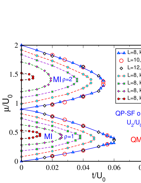
Figure 1: (Color online) The limits of the $\rho=1$ and $\rho=2$ Mott regions (MI) for different values of the temperature $kT$ and for different sizes $L$. As the temperature increases, the Mott lobes shrink and totally disappear for $kT>0.04\,U_{0}$. Outside the Mott, the system crosses over to a normal Bose liquid (NBL) and, eventually, transitions to a quasi-polarized superfluid (QP-SF) phase (see below). In the limit of zero temperature (here represented by the low temperature $kT/U_{0}=0.006$), there is a direct phase transition between a Mott phase and a superfluid.

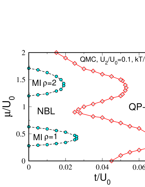
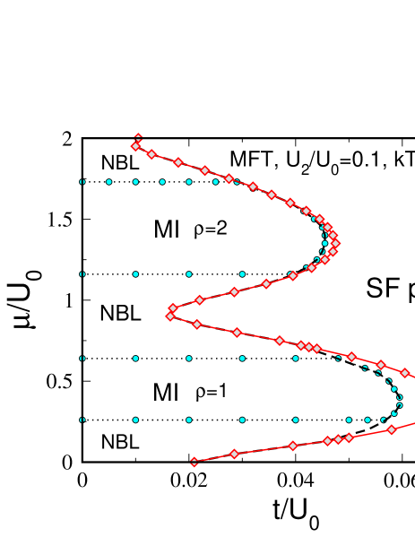
Figure 2: (Color online) Phase diagram of the system at $kT=0.03\,U_{0}$ for $U_{2}/U_{0}=0.1$. The QMC simulations (top) show that a liquid (NBL) region appears between the quasi polarized superfluid (QP-SF) phase and the Mott region. The MFT (bottom) is not able to reproduce correctly this result as it does not take into account the kinetic term in the unordered (Mott or NBL) phase. It predicts first order phase transition between the SF and the other phase at the tip of the $\rho=1$ and $\rho=2$ lobes: the region of coexistence of the two phases is limited by the dashed line and the redline with squares.

To map the phase diagram at finite temperature with QMC, we determine the limit of the Mott Insulator regions by measuring the density as a function of $\mu$ and determining the boundaries of the plateaux indicating the almost incompressible regions. As explained in Sec. IIA, although the compressibility of these regions is very small, they are not strictly incompressible due to thermal fluctuations. The evolution from MI to NBL does not show any singularity and is then simply a crossover between two different limiting behaviors, incompressible and compressible, of the same unordered phase. Strictly speaking, a truly incompressible Mott phase exists only at $T=0$ but, following convention, we will continue to refer to this finite $T$ region as a MI. To define the crossover boundary between the MI and the NBL shown in phase diagrams, we use the following criterion: when the density deviates by 1% from the total integer density we consider that the system is no longer in the MI region but in the NBL region.

Figure 1 shows the limits of the MI regions for different temperatures. As expected, the MI regions progressively disappear as the temperature is increased. The limits of the superfluid phase are located by direct measurement of $\rho_{s}$. When the system is compressible and has zero superfluid density, there is a normal Bose liquid. Fig. 2 (top) shows the QMC phase diagram of the system at a constant finite temperature. As the SF and MI regions are destroyed due to thermal fluctuations, an intermediate NBL region appears. The MFT used with success at $T=0$, where it reproduces qualitatively the phase diagram, is unable to do so at finite temperature as explained in Sec. II.1. Figure 2 (bottom) shows the MFT phase diagram where the afore mentioned problem clearly appears: the boundaries between the MI and NBL do not depend on the value of $t/U_{0}$ and the MFT is unable to give correct predictions regarding this crossover. However, the boundaries of the SF are reasonably well reproduced. A surprising result is that the transition between the unordered phase and the SF appears to be first order at the tip of the $\rho=1$ and $\rho=2$ lobes in this MFT approach. At zero temperature, only $\rho=2$ showed a first order transition. As will be shown below, for finite temperatures, this is in total contradiction with the results obtained by QMC simulations that show continuous phase transitions for $\rho=1$ and $\rho=2$. So this MFT provides incorrect description of the phase transition and of the position of the different regions at finite temperature.

For fixed integer density at zero temperature, we have a quantum phase transition (QPT) between the MI and SF phases. As expected sachdev , when the temperature is increased from zero, an intermediate compressible unordered region appears between the superfluid phase and the Mott region, namely the normal Bose liquid region (NBL). This is observed for $\rho=1$ (Fig. 3) and $\rho=2$ (Fig. 4).

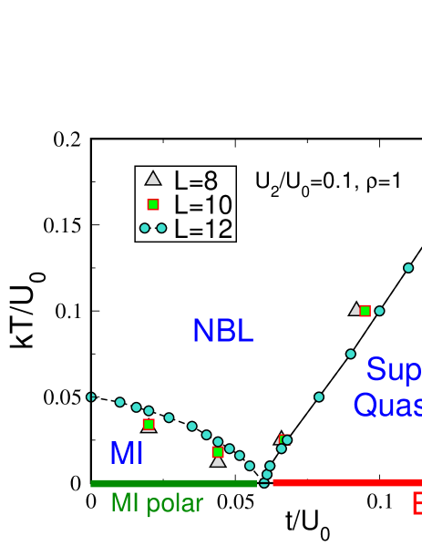
Figure 3: (Color online) The QMC phase diagram for $\rho=1$ and for different sizes showing the quantum phase transition point between the Mott insulating phase (MI) and the superfluid at $kT=0$. The finite $T$ superfluid phase does not have BEC in this two-dimensional system. The system is quasi-polarized throughout the superfluid phase, but it is not in the NBL and MI. The Mott phase is polarized at $T=0$ and should be quasi-polarized at extremely small $T$. The transition between the SF and the NBL is continuous and there is only a crossover separating NBL from MI.

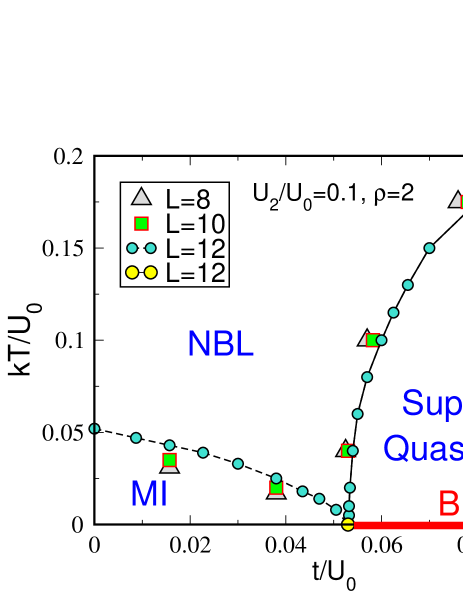
Figure 4: (Color online) The QMC phase diagram for $\rho=2$ and for different sizes showing the quantum phase transition point between the MI and the SF occurring only at $kT=0$. The superfluid phase is always quasi-polarized whereas the NBL and MI are not. The SF-NBL transition is continuous, whereas at $T=0$ the MI-SF quantum phase transition was found to be discontinuous for $U_{2}/U_{0}$ small enough deforges11 . The dash line corresponds to the case studied in Fig. 5.

As for the possible polarization of the different phases, we observe that the SF phase appears to be polarized at finite $T$ as it is at $T=0$: the histogram of the density of one of the species shows two peaks at low and high densities (see Fig. 5). However, due to the continuous symmetry in the $yz$ plane of the pseudo-spin part of the Hamiltonian Eq. (8), no LRO exists at finite $T$. Therefore, this apparent polarization is due to the finite size of the system, and is, in fact, a quasi-polarization. An intuitive way to understand this quasi-polarization is as follows: In the superfluid phase, the pseudo-spins in the $yz$ plane are stiff and appear to be mostly aligned in the same direction on a finite lattice, such as the case here. But since the symmetry is not broken, this “magnetization” direction in the $yz$ plane will drift and point in all directions. As the direction changes, so does the projection of this pseudo-spin on the $z$-axis. In other words, the polarization drifts too, and changes with time, giving the double peak structure to the polarization histogram, Fig. 5. We note that experimental systems are typically of the same sizes as the ones we study here and, therefore, this polarization drift will be present in these experiments too: The particle content of the system will change as a function of time. This quasi-polarization disappears as $T$ increases when the system undergoes a thermal BKT phase transition into the NBL. In other words, the entire SF phase is quasi-polarized but the NBL is not (see Fig. 5)

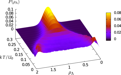
Figure 5: (Color online) Probability $P(\rho_{\Lambda})$ as a function of temperature for $L=8$, $U_{2}/U_{0}=0.1$, $\rho=2$ and $t/U_{0}=0.08$. When $kT/U_{0}<0.175$, the system is in the quasi-polarized SF phase. For $kT/U_{0}>0.175$, the system is in the unordered unpolarized phase. The temperature at which the quasi-polarization disappears is approximately the same as the temperature where $\rho_{s}$ becomes zero (see the vertical dashed line in Fig. 4). Only the SF phase is quasi-polarized.

A histogram of the polarization in the $\rho=1$ MI region shows that as soon as the temperature is increased from zero, the polarization disappears and the populations become balanced. According to the effective pseudo-spin model kuklov03 ; deforges11 , it is possible to observe quasi-polarization as in the SF phase. In this case, the coupling generating these spin correlations and the polarization of the MI is of order $t^{2}/U_{0}$. However, even for temperatures as low as $kT/U_{0}=0.01$, the system is already in the regime where correlations decay exponentially and we do not observe any QLRO at finite $T$ in the Mott region. This is confirmed by the behavior of the Green functions that is shown in Fig. 6. In Fig. 6(a) we show the anticorrelated Green function $G_{\rm a}$, Eq. (6), in the $\rho=1$ MI region as $T$ is increased. We see that as soon as $T$ becomes finite, $G_{\rm a}$ decays exponentially with distance, contrary to its constant value at long distance observed at $T=0$ deforges11 . This exponential decay of course persists in the NBL region.

In Fig. 6(b) we show $G_{\Lambda}(R)$, Eq. (5), for various $T$ values at $\rho=2$ and $t/U_{0}=0.08$ which, at $T=0$, puts the system in the SF phase. We see that for low $T$, $G_{\Lambda}$ decays slowly. This decay is expected to be a power law but the system size is too small to show that unambiguously. As $T$ is increased, the system transitions into the NBL where $G_{\Lambda}$ exhibits exponential decay clearly distinguishing the NBL and SF phases. A similar behavior is found for $G_{0}$ and $G_{\rm a}$, the latter being expected since it accompanies the presence of quasi-polarization.

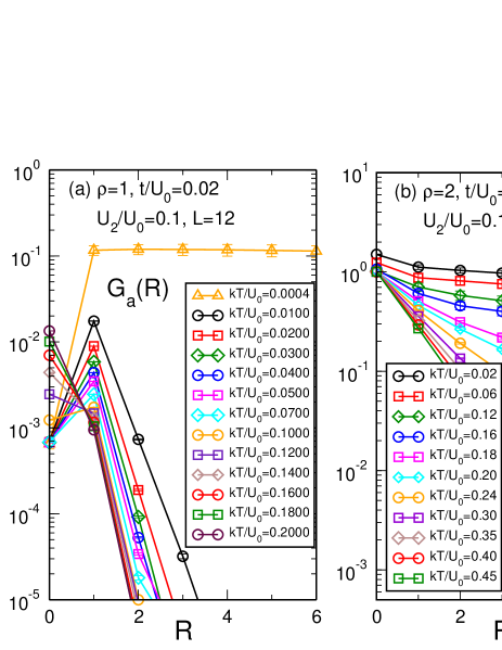
Figure 6: (Color online) Evolution of the Green functions $G_{\rm a}$, Eq. (6), in the $\rho=1$ MI and $G_{\Lambda}$, Eq. (5), in the SF as functions of distance $\bf R$ for different temperatures, with $L=12$ and $U_{2}/U_{0}=0.1$. (a) In the $\rho=1$ MI, $G_{\rm a}$ decays exponentially at finite $T$, unlike its $T=0$ behavior where it reaches a constant value deforges11 . A regime of QLRO is not observed and would occur only at very small $T$. The exponential decay persists in the NBL at higher $T$. (b) $G_{\Lambda}$ at $\rho=2$ for $T$ values taking the system from the SF to the NBL. Same case as in Fig. 5. In the SF, $G_{\Lambda}$ decays slowly as a power law, but decays exponentially in the NBL. Similar behavior is found for $G_{0}$ and $G_{\rm a}$.

III.2 Nature of the transitions

At finite temperature, $kT>0.005\,U_{0}$, the transitions between the SF and the NBL are continuous for $\rho=1$ as well as for $\rho=2$ (and of course for all other densities). Since this transition takes place at constant density and is therefore a phase-only transition, it is expected to be in the Berezinsky-Kosterlitz-Thouless universality class (BKT) for our two-dimensional system. Actually, below the critical temperature, we have two different quasi long range orders that occur: the global $U(1)$ phase QLRO associated with the superfluid behavior and the pseudo-spin one, associated with the quasi-ordering of the spins in the $yz$ plane, i.e. the so-called quasi polarization. As explained previously, these two QLRO appear simultaneously. Since the transition is BKT, we first determined the transition temperature using the universal jump of the superfluid density nelson77 , where, at the transition temperature, $T_{c}$, we have $\rho_{s}(T_{c})=kT_{c}/\pi t$. To observe this, we calculated $\rho_{s}$ as a function of temperature and determined $T_{c}(\rho_{s})$ graphically as the intersection of $\rho_{s}(T)$ with $kT/\pi t$ (see Fig. 7). We also calculated the specific heat $C$ and determined the transition temperatures $T_{c}(C_{\rm max})$ as the temperature where $C$ reaches its maximum (Fig. 7). Our QMC simulations were done for $L=8$ because $C$ is extremely difficult to calculate at low temperature for $U_{2}>0$ for larger sizes.

Figure 7: (Color online) Superfluid density $\rho_{s}$ and specific heat $C$ as functions of temperature for different values of $t/U_{0}$. The universal jump condition states that $\rho_{s}(T_{c})=kT_{c}/\pi t$. The transition temperatures are calculated independently by determining the maximum of $C(T)$.

$t/U_{0}$	$T_{c}\ (\rho_{s})$	$T_{c}\ (C_{\rm max})$
0.06	$1.49\pm 0.10$	$1.67\pm 0.15$
0.07	$1.82\pm 0.05$	$1.85\pm 0.15$
0.08	$1.99\pm 0.05$	$2.00\pm 0.15$
0.09	$2.10\pm 0.05$	$2.10\pm 0.20$
0.10	$2.19\pm 0.05$	$2.20\pm 0.20$

Table 1: Values of the transition temperatures for different values of $t/U_{0}$ for an $8\times 8$ system. $T_{c}(\rho_{s})$ is obtained from the universal jump while $T_{c}(C_{\rm max})$ from the maximum of $C(T)$. The values are in agreement and show that the universal prediction is verified. The data are taken from Fig. 7.

Table 1 compares the values of $T_{c}$ obtained from the universal jump and from the maximum of $C$. The values are in agreement confirming the universal jump hypothesis and the BKT nature of the transition and determining the transition temperature for the studied size. We did simulations for sizes up to $L=14$ to examine the effect of finite size for this transition (see Fig. 8). As expected, the transition gets sharper with increasing size. However, it is too difficult to obtain results with small enough error bars for $C$ on these large sizes.

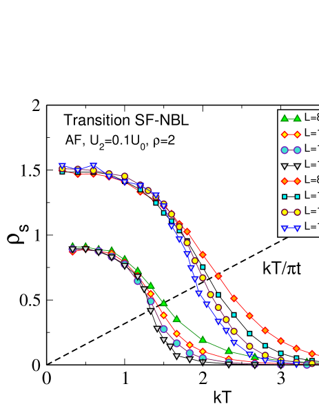
Figure 8: (Color online) Superfluid density $\rho_{s}$ as a function of $T$ for $t/U_{0}=0.06$ and $0.10$ and for different sizes $L$. The transition becomes sharper as $L$ is varied from $L=8$ to $L=14$.

As mentioned earlier, the evolution from the MI region to the NBL is a continuous crossover. A plot of the density as a function of $\mu$ shows no sign of a first order phase transition in the form of a jump in the density as one approaches the Mott plateaux (see Fig. 9). There is no phase transition between MI and NBL since, in addition to the absence of a first order transition, no symmetries are broken. Then, at finite temperature, there is only a crossover between the MI and the NBL and not the phase transition predicted by MFT.

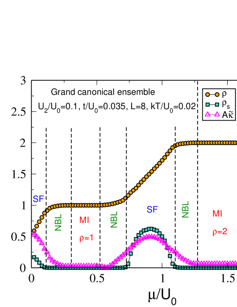
Figure 9: (Color online) $\rho$, $\rho_{s}$ and ${\tilde{\kappa}}$ as functions of $\mu$. As one goes from the MI to the NBL, the density varies continuously indicating a crossover between the two regions. The two regions are distinguished by the integer/non-integer value of the density and by the larger value of the local compressibility ${\tilde{\kappa}}$ in the liquid. The superfluid phase has nonzero $\rho_{s}$ and a much larger local compressibility than both the MI and NBL. ${\tilde{\kappa}}$ has been multiplied by an arbitrary factor $A$ for better visibility.

At zero temperature, we have shown deforges11 that the Mott-SF transition is always second order for $\rho=1$ but is first order near the tip of the $\rho=2$ Mott lobe when $U_{2}/U_{0}$ is small enough, for example $U_{2}/U_{0}=0.1$. Hence, while it is easy to imagine that the continuous NBL-SF transitions observed at moderate temperatures persists at low temperature for $\rho=1$, the $\rho=2$ case where the behavior is different at zero and finite temperatures requires a separate study for the low temperature regime. Probing temperatures as low as $kT=0.005U_{0}$ (see Fig. 10), the transition still appears continuous, which is to be compared with the temperature at which the MI region is destroyed $kT\approx 0.05U_{0}$ (see Figs. 3 and 4). Although it cannot be excluded that the transition is discontinuous in a small range of temperatures, this range would be extremely narrow. In order to observe the first order QPT in our previous work deforges11 we used temperatures that were of order $kT/U_{0}\simeq 10^{-3}$. The transition then appears discontinuous only at extremely low temperatures.

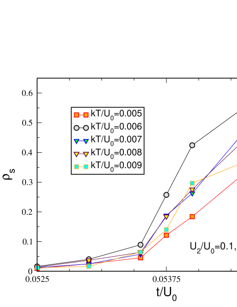
Figure 10: (Color online) Transition from the normal Bose liquid to the superfluid phase at low temperatures. The transition always appears continuous for low temperatures. The discontinuity is only found in the zero temperature regime ($kT<10^{-3}U_{0}$).

IV $U_{2}<0$ case

It was shown for $U_{2}<0$ deforges11 that all the phases are unpolarized and that transitions between the different phases are all continuous in the $T=0$ limit. The coherent anticorrelated movements are present in the $\rho=1$ and in the $\rho=2$ Mott phases.

Proceeding as in the $U_{2}>0$ case, we determine the boundaries of the Mott regions at finite $T$, Fig. 11, by calculating the density and the boundary of the superfluid region by measuring $\rho_{s}$. In this case, we chose not to present results from MFT since it shows the same limitations as in the $U_{2}>0$ case. We obtain the phase diagram for $\rho=1$ (shown in Fig. 12) and a similar one for $\rho=2$ (not shown here). Similarly, we used histograms of the density similar to Fig. 5 to confirm that all these phases remain unpolarized at finite temperature as they are at zero temperature. The absence of polarization at $T$ can be understood qualitatively from Eq. (8). For the present case, $U_{2}<0$, the last term in Eq. (8) favors the alignment of the spins along the $x$-axis in the low $T$ phase. Consequently, the polarization, $S^{z}$, is always zero.

As in the $U_{2}>0$ case we observe a slow decay of the Green functions $G_{\sigma}$ in the superfluid phase and the transition is shown to be of the BKT type using the universal jump argument (see Table 2).

$t/U_{0}$	$T_{c}\ (\rho_{s})$	$T_{c}\ (C_{\rm max})$
0.06	$1.85\pm 0.05$	$1.75\pm 0.10$
0.07	$2.00\pm 0.05$	$2.00\pm 0.10$
0.08	$2.10\pm 0.05$	$2.05\pm 0.05$
0.09	$2.14\pm 0.05$	$2.16\pm 0.05$
0.10	$2.18\pm 0.05$	$2.15\pm 0.05$

Table 2: Values of the SF to NBL transition temperatures for different values of $t/U_{0}$ and for a $L=12$ size for $U_{2}/U_{0}=-0.1$ and $\rho=2$. Similar to Table 1.

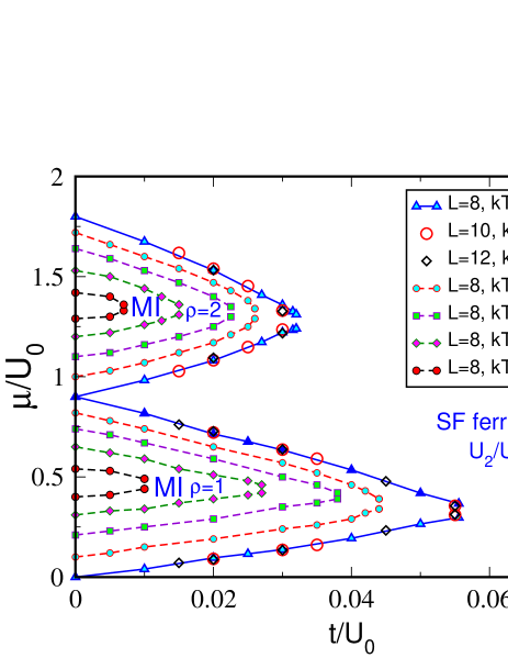
Figure 11: (Color online) The limit of the $\rho=1$ and $\rho=2$ Mott regions (MI) for different values of the temperature $kT$ and for different sizes $L$ in the $U_{2}<0$ case. As in the positive $U_{2}$ case, the Mott phases disappear for $kT>0.04U_{0}$. In the $T=0$ limit, there is a direct transition between the MI and SF.

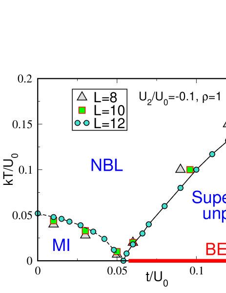
Figure 12: (Color online) The phase diagram for $\rho=1$ in the $U_{2}<0$ case. All phases are unpolarized and the SF-NBL transition at finite temperature as well as the MI-SF transition at zero temperature are continuous. A similar phase diagram is observed for $\rho=2$.

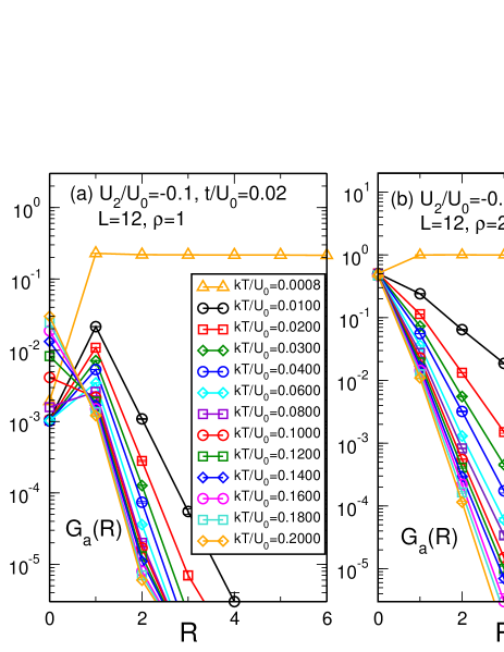
Figure 13: (Color online) The anticorrelated Green functions in the $\rho=1$ (a) and $\rho=2$ (b) Mott regions for negative $U_{2}$. In both cases, the long range order of the anticorrelated movements that was present at $T=0$ is lost even for very small temperatures.

We also examined the anticorrelated Green function $G_{\rm a}$ in both $\rho=1$ and $\rho=2$ MI regions at various temperatures. In the zero temperature limit, both these phases exhibit nonzero values of $G_{a}$ at long distances. This is expected in both cases, considering the pseudo-spin Hamiltonian. Neglecting the kinetic energy, for $U_{2}<0$, the energy is minimized by maximizing $(S^{x}_{\bf r})^{2}$ on each site. For $\rho=1$ and $\rho=2$, there are two degenerates states that achieve this: the $S^{x}_{\bf r}=\pm 1/2$ for $\rho=1$ and the $S^{x}_{\bf r}=\pm 1$ for $\rho=2$. These degenerate ground states are coupled by second order hopping processes which lift this degeneracy through coherent anticorrelated movements deforges11 . In Fig. 13, we show $G_{\rm a}$ in the $\rho=1$ and $\rho=2$ MI regions for different temperatures. As expected, the phase coherence once again completely disappears rapidly as the temperature is increased from zero and we do not observe any sign of quasi long range phase coherence in the MI region, as well as in the NBL phase.

V Conclusion

Studying a bosonic spin-$1/2$ Hubbard model at finite temperature and comparing to the $T=0$ case, we find that the effect of temperature is dramatically different depending on the phase we consider. The superfluid phases are essentially unchanged by raising the temperature: The long range order present at $T=0$ is transformed into QLRO. On the other hand, the MI regions are drastically modified as the polarization that occurs in certain cases is almost immediately wiped out by thermal fluctuations: low temperature quasi polarized states are not found in the regime of temperatures we studied.

This is due to the fact that the energy scales associated with the polarization of the system take different values in these different phases. In the MI regions, the polarization is due to the coupling between different low energy degenerate Mott states, as emphasized by the pseudo-spin theory kuklov03 . These couplings are of order $t^{2}/U_{0}$ and the pseudo-spin quasi-ordering vanishes very rapidly with temperature. On the other hand, in the superfluid, the energy scale associated with the coupling of pseudo-spins is obviously much larger. While it is not possible to specify this scale as precisely as in the Mott phases, due to the itinerant nature of the particles in the superfluid regime, a simple argument shows that it is of order $U_{2}$: whenever the particles enter the superfluid phase and adopt delocalized states, they overlap; there is an interaction cost which is then of order $U_{0}$ for identical particles and $U_{0}+U_{2}$ for different ones. This favors having the particles mostly of the same type for $U_{2}>0$ and leads to a quasi polarization. For $U_{2}<0$, the interaction favors having a mixture of particles and gives a system without any sign of polarization. In both cases, the energy scale is typically $|U_{2}|$

The finite temperature phase diagram presented here is important for the proper interpretation of experimental realization of this and related systems using ultra-cold atoms loaded on optical lattices. Such experiments are, of course, always at finite temperature. Similarly to what happens for fermions, we observe that the spin correlations in the Mott phases will be very difficult to access experimentally as the associated energy scales are very small and as the correlations are almost immediately wiped out by thermal fluctuations. On the other hand, due to the relatively small sizes of experimental systems and to its larger associated energies, the quasi-ordering of spins in the superfluid phase should be immediately visible experimentally and indistinguishable from true polarization of the system. In a finite size system, one would expect to observe a slow drift of the polarization as the $yz$ symmetry of the system is restored over time.

From a more technical point of view, we have elucidated the limitations of the MFT commonly used in the literature. We found that it is unable to distinguish correctly the MI and NBL regions. The MFT does predict reasonably well the NBL-SF boundaries but not the nature of the transition which is sometimes predicted to be of first order whereas direct QMC simulations, and symmetry considerations, show that it is in the BKT universality class. Furthermore, we found that MFT predicts direct first and second order transitions at finite $T$ between the MI and SF phases which QMC shows do not exist, (see Figs. 3, 4, 12). Similar incorrect MFT behavior was found for the spin-$1$ model and the same caveats should be applied for example in Ref.Pai08 .