Optimal Cosmic-Ray Detection for Nondestructive Read Ramps

Abstract

Cosmic rays are a known problem in astronomy, causing both loss of data and data inaccuracy. The problem becomes even more extreme when considering data from a high-radiation environment, such as in orbit around Earth or outside the Earth’s magnetic field altogether, unprotected, as will be the case for the James Webb Space Telescope (JWST). For JWST, all the instruments employ nondestructive readout schemes. The most common of these will be “up the ramp” sampling, where the detector is read out regularly during the ramp. We study three methods to correct for cosmic rays in these ramps: a two-point difference method, a deviation from the fit method, and a y-intercept method. We apply these methods to simulated nondestructive read ramps with single-sample groups, and varying combinations of flux, number of samples, number of cosmic rays, cosmic-ray location in the exposure, and cosmic-ray strength. We show that the y-intercept method is the optimal detection method in the read-noise-dominated regime, while both the y-intercept method and the two-point difference method are best in the photon-noise-dominated regime, with the latter requiring fewer computations.

1. Introduction

Advances in technology that allow us to observe fainter objects, build more complex systems, and send telescopes further into space have challenged us to continue to improve our calibrations. This includes detection methods for cosmic rays (CRs) or any charged particle that adds a jump to the data. JWST’s orbit at the second Earth-Sun Lagrange point (L2), which allows passive cooling of the telescope to $\sim$50 K, puts it outside the protective mantel of the Earth’s magnetic field. This could make CRs a serious problem. Furthermore, newer infrared telescopes will have a lower read-noise, and thus we will detect lower CRs. Finally, long observing times will be necessary to complete many of the scientific goals of the JWST, causing CRs to be an even larger problem. From a study by Robberto (2009a) we can calculate that in every 2000 s, on average, 13% of the pixels on the JWST HgCdTe detectors and 25% of the pixels on the JWST Si:As detectors will be affected by CRs. These values could be even greater, since this study does not take into account secondary particles. For comparison, onboard measurements of the NICMOS camera on the HST show that about 10% of the pixels show a CR hit for every 2000 s of integration (Viana and Wiklind et al., 2009). These CRs will include low-energy CRs from secondary particles and the Sun, and higher-energy galactic CRs (Robberto, 2009c). Clearly, a reliable method to detect both low- and high-energy CRs is needed.

In this article we will discuss CR detection methods for infrared data, which use nondestructive read ramps. Offenberg et al. (2001) found that in order to correct for CRs, the nondestructive readout scheme was most efficient. By integrating the charge on each pixel in this way it is possible to calculate the slope of these ramps in counts per time to get the flux of the sky (Rieke 2007). We refer to the integrated charge as a ramp made up of a specified number of samples. We discuss the slope of these ramps as the calculation of the flux. Finally, a CR affects the ramp between samples, however we use ‘sample number’ to refer to the first sample after the CR hit.

Correcting for CRs in ramps is not a new problem (Offenberg et al., 1999). However, the advent of large nondestructive arrays in orbit coupled with ground-based processing of the ramps means, when it comes to calculating the slope of ramps, that there are more options available for CR detection. In addition to CRs, noise is added to the data by the detector and readout electronics as well (Fanson 1998, Tian et al. 1996, Rieke 2007). In this article we focus on photon-noise and read-noise for our correlated and uncorrelated noise, respectively; however, we are not restricted to just these two terms. The work in this article is general and can account for any correlated and uncorrelated noise sources. Therefore, our question is, What is the best we can do at finding CRs in a ramp, given the noise in the ramp?

To understand and test various CR detection methods for ramps, we simulate infrared data as described in Section 2. Anytime a slope is calculated for the preceding process or for the CR detection methods, we do so using linear regression for data with correlated and random uncertainties (in consideration of the photon-noise and the read-noise, respectively), as described in Section 3. In Section 4 we propose three techniques to detect CRs. The first is a two-point difference method, the second is a deviation from the fit method, and the third is a y-intercept comparison. There are various conditions that can hinder/aid in CR rejection (e.g., number of samples, slope, number of CRs, size of CRs, and location of CRs); therefore, we aim to study combinations of these and to find which algorithm behaves the best under different conditions. These results are presented in Section 5. A discussion on our findings is in Section 6. Concluding remarks can be found in Section 7.

2. Simulating Nondestructive Read Ramps

In order to test how well a CR detection method works, we have to test the method on a known CR. For that reason, we have simulated ramps with photon-noise and read-noise added in, to which we can either add CRs with known location in the exposure and known amplitudes or leave the ramps clean (CR-free). We build these ramps with the slope, y-intercept, number of samples, time between samples (sample time), and read-noise as inputs, using parameters given in Table 1 as guidelines (slope and number of samples will be changed in this study). The only value that is instrument-specific is the read-noise, which was chosen to match the expected value of the Mid-Infrared Instrument (MIRI) on the JWST. Note that we do not group any of the samples by taking a weighted average or coadding. Furthermore, we assume uniform sampling (i.e., constant time between samples), as that is what is used by the JWST and also so that calculations are more efficient. We also assume that a nonlinearity correction has already been performed with no error, and we do not account for the effects of quantization noise. Although we are simulating MIRI detector parameters, this is only an example. The methods discussed in this article will apply to any other nondestructive read data, including those for the JWST near-infrared detectors (Near-Infrared Camera [NIRCam] and Near-Infrared Spectrograph [NIRSpec]) the HST infrared detectors (Wide Field Camera 3 - IR [WFC3-IR] and Near-Infrared Camera and Multi-Object Spectrometer [NICMOS]) and ground-based detectors, by simply changing the values in Table 1. If the data you would like to simulate do included grouped samples, however, some revisions will have to be made.

Parameters	Values
Slope	70.0 $e^{-}$/s
Y-Intercept	21000.0 $e^{-}$
Number of Samples	40
Sample Time	27.7 s
Read Noise	16.0/$\sqrt{8}$ $e^{-}$/sample

Table 1Parameters Used to Create MIRI Ramps.

At time $t=0$ the counts $y_{0}$ are equal to the y-intercept. This is not considered part of the ramp, because $t=0$ is when the reset occurred, but we start reading at time equal to one sample time, $t_{1}$.

Each signal is comprised of the counts from the previous signal plus the additional signal, the photon-noise from the additional signal, and the read-noise. To construct the ramps, we follow this procedure:

1. For each ramp calculate the expected signal (i.e., no noise, clean), $s_{e}$, defined as

   $$s_{e}\equiv mt_{s},$$ (1)

   where $m$ is the input slope, and $t_{s}$ is the sample time.

2. For each sample calculate the sum of the expected signal and the unique photon-noise of this signal ($s_{e}+\sigma_{n_{p}i}$) from a Poisson distribution with $\lambda=s_{e}$. Add this to the signal from the previous sample (or y-intercept if it is the first sample). This step is shown in equation 2. Since we have only added the correlated noise, and we still need to add the uncorrelated noise, we have called the signal $y_{i}^{*}$ instead of $y_{i}$).

   $$y_{i}^{*}=y_{i-1}^{*}+s_{e}+\sigma_{n_{p}i}.$$ (2)

3. If there are to be one or more CRs to the ramp, simply add the electrons with the expected signal:

   $$y_{i}^{*}=y_{i-1}^{*}+s_{e}+\sigma_{n_{p}i}+CR_{mag},$$ (3)

   where $CR_{mag}$ is the magnitude of the CR.

4. Read noise, denoted by $n_{r}$, is due to readout electronics; consequently, it is uncorrelated. Therefore, when all samples are populated, add a unique read-noise, $\sigma_{n_{r}i}$, to each sample (equation 4):

   $$y_{i}=y_{i}^{*}+\sigma_{n_{r}i}.$$ (4)

   For each sample $\sigma_{n_{r}i}$ is taken from a Gaussian with $n_{r}$ as the standard deviation.

The uncertainties for the samples in the ramp are calculated by adding the photon-noise and read-noise in quadrature:

$$\sigma_{y}=\sqrt{n_{r}^{2}+n_{p}^{2}},$$ (5)

where $n_{p}$ is the Poisson noise of the expected signal in the ramp; thus, $n_{p}=\sqrt{mt_{s}}$, and $n_{r}$ is taken from Table 1. We have chosen to give each sample equal weighting, rather than choosing the photon-noise to be the Poisson noise of the counts in the ramp, so that we can improve our results by avoiding a bias based on sample number.

3. Linear Fit Algorithm for Data with Correlated Errors

For two of the three CR detection methods, it is very important that we use the best calculation of the slope and y-intercept. Therefore we must use all information including correlated and uncorrelated errors. Gordon et al. (2005) explains how to take into account both correlated and uncorrelated errors for the slope and y-intercept uncertainties, and here we describe how to include this information for the fit as well, using matrix notation and specifically making use of the covariance matrix. For a refresher on calculating a linear fit using matrices as well as the use of the covariance matrix, see Hogg et al. (2010). Every time a slope is calculated in the CR detection methods described in this article, we do so using this method.

The real power of using matrix notation comes from the covariance matrix, $\bf{C}$, as it includes information about the degree of correlation between samples. Furthermore, the slope and y-intercept uncertainties resulting from using this covariance matrix automatically take into account the correlated and uncorrelated errors, provided they are included in the covariance matrix. $\bf{C}$ is defined as:

$$\bf{C}=\left[{\begin{array}[]{cccc}\sigma^{2}_{y_{1}}&c_{1,2}&...&c_{1,N}\\ c_{2,1}&\sigma^{2}_{y_{2}}&...&c_{2,N}\\ ...&...&...&...\\ c_{N,1}&c_{N,2}&...&\sigma^{2}_{y_{N}}\\ \end{array}}\right].$$ (10)

The values on the diagonal of $\bf{C}$ are the uncertainties of the $y_{i}$, whereas the off-diagonal elements are the covariance between the different $y_{i}$. If the data are uncorrelated, then the off-diagonal matrix elements are all zero, $c_{i,j}=0,i\neq j$. However, we do have correlated data due to the photon-noise.

When constructing $\bf{C}$ for correlated errors, we follow the logic of Fixsen et al. (2000) and think of $\bf{C}$ as the sum of two matrices: one for the photon-noise, $\bf{P}$, and one for the read-noise, $\bf{R}$. Fixsen et al. (2000) define these matrices for the case where the data are the two-point difference of the samples (the photon-noise is not correlated, and the read-noise is correlated). However, for fitting a line to the individual samples, it is just the opposite. The read-noise is uncorrelated, and thus $\bf{R}$ is just $n_{r}^{2}$ on the diagonal and zero elsewhere.

The diagonal of $\bf{P}$ is $n_{p}^{2}$, just as it would be for uncorrelated data, but since the photon-noise is correlated, the off-diagonal elements are not zero. An estimate of all of the photon-noise in $y_{i}$ is the photon-noise added to each sample multiplied by $i$ (i.e., $in_{p}$). The correlation between samples $y_{i}$ and $y_{j}$ is the photon-noise that is in $y_{i}$ that is also in $y_{j}$. The elements in $\bf{P}$ that represent this correlation are $p_{i,j}$ and $p_{j,i}$. Consider $y_{2}$ and $y_{3}$, where the photon-noise they share would be the photon-noise in $y_{2}$ ($2n_{p}^{2}$), plus the photon-noise in the first read, $p_{1,1}$. Thus,

$$p_{i,j}=p_{j,i}=kn_{p}^{2}+p_{1,1},$$ (11)

where

$$k=\Big{\{}{\begin{array}[]{cc}j,&j<i\\ i,&i<j\\ \end{array}}.$$ (14)

If $p_{1,1}$ is included in the background, then it is set to zero. We can estimate $n_{p}$ using the slope as we did in Section 2: $n_{p}=\sqrt{s_{e}}$. This initial calculation of the slope for $s_{e}$ (eq. 1) is done before any CR correction and without taking into account correlated errors.

This technique accounts for the diagonal elements as well. Therefore,

$$\begin{array}[]{lr}c_{i,j}=n_{p}^{2}k+p_{1,1}+n_{r}^{2}&i=j,\\ c_{i,j}=n_{p}^{2}k+p_{1,1}&i\neq j,\\ \end{array}$$ (17)

where $n_{r}$ is the read-noise.

An equation for the noise in a ramp has previously been derived in nonmatrix form in Rauscher et al., 2007; for an independent derivation and the correct final formula, see (Robberto, 2009b). Rauscher et al. formula (eq. (1) in that article, see erratum) has the benefit that it takes into account grouped samples. However, the benefit of using matrix notation with a covariance matrix is that we can add other noise terms easily by calculating the appropriate covariance matrix (like we did for P and R) and sum all to get C. It would be more difficult to add other noise terms to the Rauscher et al. (2007) equation, and like our method here, they only include read-noise and photon-noise.

3.1. Validating with Simulations

To demonstrate how well this calculation of the uncertainties fits simulated data, we followed the idea from Figure 16 in Gordon et al. (2005) and simulated 10,000 ramps each with read-noise only, photon-noise only, and both, then we used the covariance matrix to calculate the y-intercept and slope uncertainties. This is given in Figure 1. The dashed and dotted lines are the uncertainties with read-noise and photon-noise only, respectively. The solid lines are the uncertainties in the ramps where both read-noise and photon-noise were added. Notice that you can see where the transition is between the read-noise-dominated regime and the photon-noise-dominated regime using these plots. The circles are the uncertainties calculated using the method described in Section 3, which fit the data perfectly.

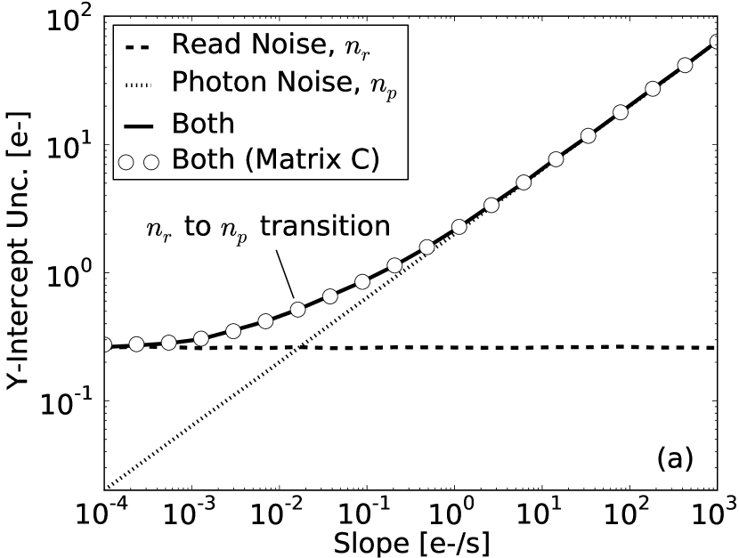
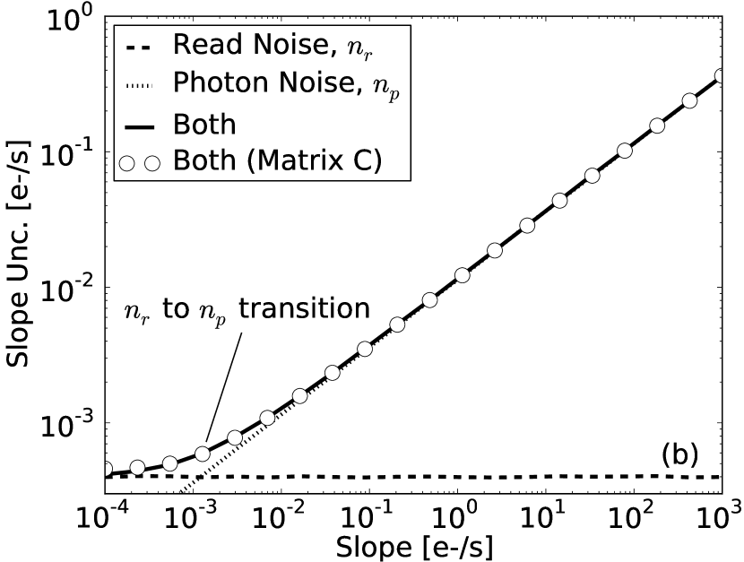
Figure 1.— Calculation of the uncertainties for the y-intercept (a) and the slope (b) using the method described in Section 3. Following the idea from Figure 16 in Gordon et al. (2005), for 10,000 each, we generated ramps with read-noise only, photon-noise only, and then both. The uncertainties in the y-intercept and slope given by the data are plotted by the dashed, dotted, and solid lines. Then using correlated and uncorrelated components in the covariance matrix (e.g., including both read-noise and photon-noise) we calculated the corresponding uncertainties shown by the circles. These calculations match the data perfectly. Furthermore, this plot also shows where the transition is between the read-noise-dominated regime and the photon-noise-dominated regime.

In addition to using a covariance matrix, other popular methods to fitting a line to ramps have used uncertainties as the weights (1/$\sigma^{2}$), equal weights, or optimum weights, as discussed in Fixsen et al. (2000). To demonstrate how these methods compare, we simulated 10,000 ramps, each with the same input slope (before the noise was added) and then tried to retrieve these slopes using the various weighting schemes (Figure 2). The standard deviation in the slope fits is plotted in Figure 2 (a). We see that the covariance matrix and optimal weighting result in a higher signal-to-noise ratio (S/N) than the other two methods. Optimal weighting estimates a covariance matrix, so it is expected that they show similar results. In Figure 2 (b) we show the ratio of the average calculated slope to the input slope, with unity subtracted. Note that the curve in this plot is nonsmooth due to the finite number of trials. The error on the slope calculation is very small, with the calculated slope at most 0.004% from the input slope. For various slopes we made a histogram of the distribution of these ratios and found that they were symmetric and centered on the average. Therefore, optimal weighting and using a covariance matrix with correlated and uncorrelated errors produces a lower standard deviation of the results, while all methods produce a similar slope estimate with 10,000 trials.

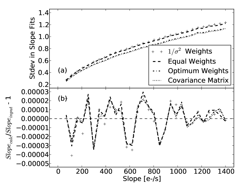
Figure 2.— (a) Standard deviation of slope fits versus input slope, for various weighting schemes to point out that using the covariance matrix has lower noise (though it is very similar to optimum weighting, as optimum weighting is an estimate of the covariance matrix). (b) Calculated slope to input slope ratio minus one for the same methods. All methods show the same bias; therefore, the difference lies only in the S/N shown in (a).

4. CR Detection Methods

All three CR detection methods have a unique algorithm. However, all follow the same procedure to calculate a slope once the CRs are found, which we now outline:

1. Detect CRs, always looking for the largest outliers first.

2. Calculate the slope for the resulting ramp segments before and after the CR events (we will refer to these as “semiramps” from here on, following Robberto, 2008).

3. Calculate the final slope of the entire ramp. If there is one CR or more, do this by taking the weighted average of the slopes of the semiramps (see also the discussion in Section 6).

Furthermore, for all methods we use the absolute difference so that we remove outliers in both directions and do not bias the data (Offenberg et al., 1999, 2001). However, if larger rejection thresholds are used, and therefore there are no longer as many outliers (i.e., only picking up the strongest CRs), then one-sided clipping would work just as well (Windhorst et al., 1994).

4.1. Two-Point Difference Method

With the nondestructive readout method, algorithms for CR detection include computing the two-point differences. Offenberg et al. (1999) and Fixsen et al. (2000) describe versions of this method, though both use only one rejection threshold for all cases (5$\sigma$ and 4.5$\sigma$, respectively). Another version was used in the Multiband Imaging Photometer (MIPS) data reduction algorithm for Spitzer (Gordon et al., 2005). We describe a variant of this technique here.

For the two-point difference method (hereafter 2pt diff), we calculate the two-point differences between the counts in each set of adjacent samples. The largest outlier is flagged as a CR, given that it fulfills the rejection criteria:

$$\frac{|d_{i}-\mu_{d}|}{\sigma_{d}}>r_{t},$$ (18)

where $d_{i}$ is the difference between the science data $y_{i+1}$ and $y_{i}$, $\mu_{d}$ is the median of $d$, $\sigma_{d}$ is the uncertainty of $d$, and $r_{t}$ is the rejection threshold. The median is used because it is more robust than the mean when there are outliers in the data (Press et al., 1986; Offenberg et al., 1999). The median can become a problem if there is quantization noise (i.e., if the slope of the ramp were 0.07 $e^{-}$/s), however we do not take into account quantization noise in this article. Once a CR is identified, the $d_{i}$ that includes the CR is removed, and the process is repeated on the remaining $d_{i}$ until no more CRs are found. This method is depicted in Figure 3.

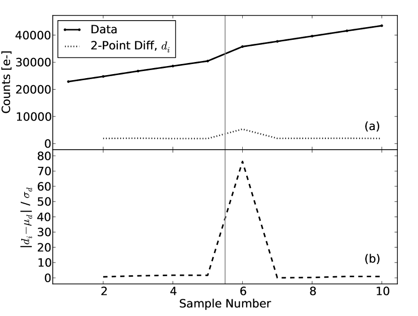
Figure 3.— 2pt diff method. (a) Solid line and points are the data, $y_{i}$, and the dotted line is the two-point differences, $d_{i}$, of this data. (b) Dashed line is the ratio in equation 18 which will be compared with the rejection threshold, $r_{t}$. The vertical line shows the interval where the CR hit.

When calculating the uncertainty in $d$, $\sigma_{d}$, the most obvious solution would be to use the standard deviation. However we have found that this does not work well for ramps with a low number of samples ($\sim 5$). We can improve $\sigma_{d}$ by using the photon-noise and read-noise added in quadrature. The photon-noise can be calculated as Poisson noise, but since we are dealing with the two-point difference we use the charge accumulated since the last sample, rather than the total charge in a sample, so we use $\sqrt{s_{e}}$. Since a CR can contaminate a slope calculation, we can use $\mu_{d}$ to estimate $s_{e}$. Therefore $n_{p}=\sqrt{\mu_{d}}$, and

$$\sigma_{d}=\sqrt{n_{p}^{2}+2n_{r}^{2}},$$ (19)

where the factor 2 is due to the read-noise from each of the two samples.

4.2. Deviation from the Fit Method

The method we will refer to as the deviation from the fit method (hereafter dev from fit), is the one used by NICMOS (Dahlen et al., 2008) and WFC3 (Dressel, 2010). To use this method we fit a line to the ramp using a covariance matrix as described in Section 3. Then, for each sample, we calculate the difference to the fit as a ratio to the uncertainty in the counts:

$$dev_{i}=\frac{y_{i}-f_{i}}{\sigma_{y}},$$ (20)

where $f_{i}$ is the fit at sample $y_{i}$, and $\sigma_{y}$ is the uncertainty in each sample, defined in equation 5.

We then take the first difference of these ratios, and look for the largest. If it satisfies the criteria:

$$|dev_{i+1}-dev_{i}|>r_{t},$$ (21)

then $y_{i+1}$ is flagged as a CR. The ramp is then split into semiramps, and this method is applied again to the resulting semiramps.

The dev from fit method is illustrated in Figure 4. Note that the background level is not at zero as it was for the 2pt diff method, but $\sim 10$. The reason for the nonzero background is that while the median (which would exclude the CR) is subtracted in the 2pt diff method, in the dev from fit method the fit is subtracted, which includes the CR in its calculation. Furthermore, in the presence of a CR, the slope will be overestimated and, therefore so will the photon-noise. Finally, the peak is at a ratio of $\sim$60, whereas both the 2pt diff and y-int methods (as we will see) peak at ratios of $\sim$80.

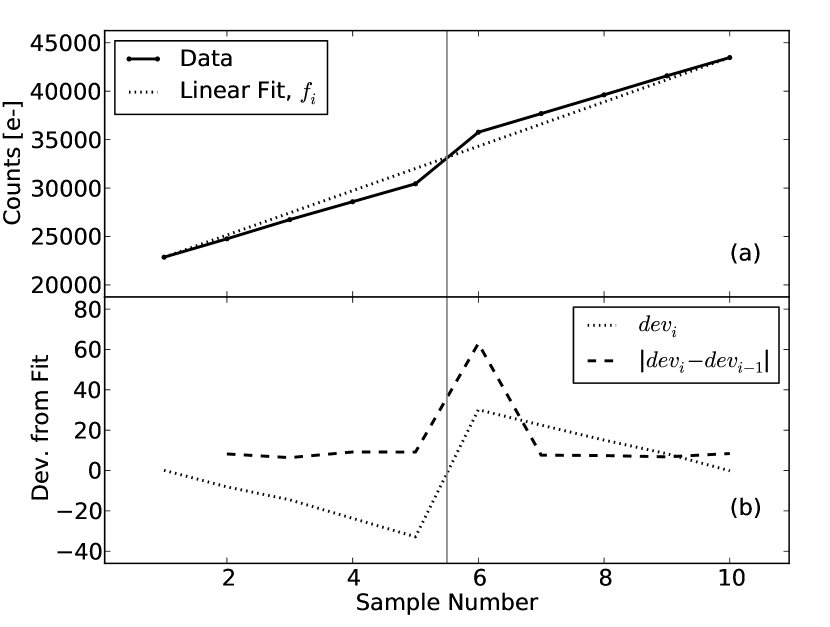
Figure 4.— dev from fit method. The solid line and points are the data, $y_{i}$ and the dotted line is the linear fit made up of points, $f_{i}$. In the lower panel the dotted line is the ratio of the difference between the fit and the data to the uncertainty, $dev_{i}$. The dashed line is the two-point differences of the $dev_{i}$. This is what will be compared with the rejection threshold, $r_{t}$. The vertical line shows the interval where the CR hit.

4.3. Y-Intercept Method

The idea for the y-intercept method (hereafter y-int) comes from the MIPS data reduction algorithm (Gordon et al., 2005). The details we describe here are a variant of that method. For the y-int method, we step through each sample and assume that there is a CR there (the first sample is skipped). We fit a line to the semiramps before and after the sample with the assumed CR, using a covariance matrix as described in Section 3. At each sample, the x-axis is shifted so that the y-intercept is located at the sample number of the assumed CR. The only exception is when we assume that there is a CR in the second sample. Since we cannot calculate a y-intercept for only one point, we shift the x-axis to the first sample, and use the counts in that sample as the y-intercept, and take the read-noise as the uncertainty. We do the mirror to this when assuming that there is a CR in the last sample. Then, we take the ratio of the absolute differences between the two y-intercepts ($b_{1}$ and $b_{2}$) to the expected uncertainty, $\sigma_{b}$ (equation 22).

$$\frac{|b_{2}-b_{1}|}{\sigma_{b}}>r_{t}$$ (22)

After stepping through every sample, we look at the sample with the largest ratio. If this ratio is larger than a given $r_{t}$, then we flag that sample as a CR. The process is repeated on the resulting semiramps. The method is depicted in Figure 5.

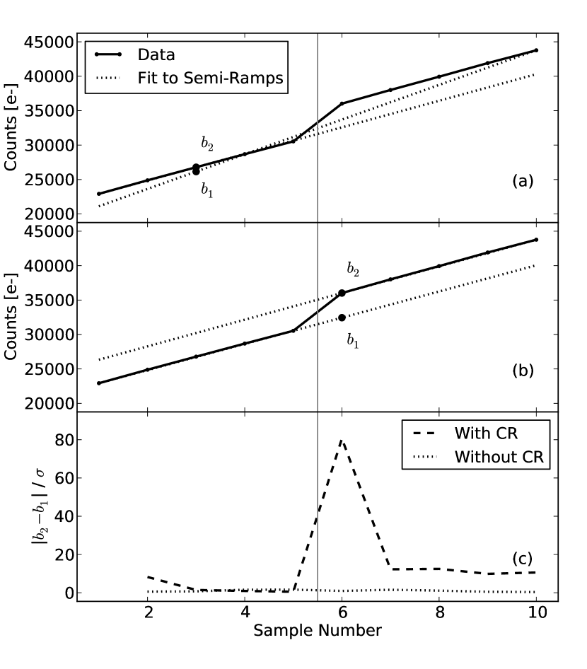
Figure 5.— y-int method. (a) Counts and two linear fits as it would look when assuming that the CR is in sample 3. The solid line and points are the data, and the dotted lines are the linear fits to the semiramp before and after the assumed CR. The two y-intercepts, $b_{1}$ and $b_{2}$ are highlighted with dots and labeled. (b) Assuming the CR is in sample 6 (which indeed it is). (c) Results after stepping through the entire ramp assuming a CR is in each sample. Plotted is the ratio of the absolute difference between the y-intercepts to the uncertainty, which must be above the rejection threshold, $r_{t}$, to be counted as a CR. The interval where the CR hit is shown by the vertical line.

The expected uncertainty, $\sigma_{b}$, is calculated from the y-intercept uncertainty from the read-noise and the y-intercept uncertainty from the photon-noise added in quadrature. There are two read-noise components, $n_{r_{1}}$ and $n_{r_{2}}$, one from the ramp before the assumed CR, and one from the ramp after. These read-noise terms are calculated by setting the covariance matrix, $\bf{C}$, to the read-noise matrix, $\bf{R}$, and recalculating the y-intercept uncertainty. The photon-noise component is calculated as $n_{p}=\sqrt{s_{e}}$. Since in the y-int method we are dealing with two ramps, we take the weighted average of the slopes to get $s_{e}$, just as we would if there were actually a CR found at the assumed location. Therefore,

$$\sigma_{b}=\sqrt{n_{p}^{2}+{n_{r_{1}}}^{2}+{n_{r_{2}}}^{2}}.$$ (23)

In Figure 5 (c) the dashed line representing equation 22 is hovering around zero before the CR detection, and then afterward it increases to $\sim$10. This effect comes from the difference between the y-intercepts. It is caused by the fact that we shift the x-axis to the sample with the assumed CR, whereas if we shift it to the sample before the CR (as we do for a CR in the second sample, notice that there the ratio is $\sim$10), then the difference between $b_{1}$ and $b_{2}$ before the actual CR would be greater than after the actual CR.

5. Results

To compare the success of each method at finding CRs, we look at both the fraction of CRs found and the false detection rate, which we define as the ratio of the number of false detections to the number of possible false detections. The number of possible false detections is calculated as the number of samples minus one, minus the number of true CRs, times the number of trials.

We look at simulated ramps with 5, 10, 20, 30, and 40 samples, with CRs of 20 different magnitudes from 0 to 250 $e^{-}$ (all CRs with magnitudes $>$250 $e^{-}$ are found with all methods), and with slopes of 0.0 $e^{-}$/s, 0.7 $e^{-}$/s, 3.5 $e^{-}$/s, 7.0 $e^{-}$/s, 35.0 $e^{-}$/s, and 70.0 $e^{-}$/s, with one, two, or three CRs, and with the CR located in the beginning, middle, and end of the ramp (e.g. for a ramp with 40 samples, we inserted a CR in the $3^{rd}$, $10^{th}$, $20^{th}$, $30^{th}$, and the $35^{th}$ sample). We then simulate 10,000 ramps for each combination, and apply each method to each ramp to compare the results. For all trials, the rejection threshold, $r_{t}$, is chosen such that the rate of false detections is the same for all methods (a rate of 5% was chosen). In this way we can best compare how well they find the CRs.

5.1. The Rejection Threshold, $r_{t}$

Each of the CR detection methods has a different criterion (see equations 18, 21, and 22), which, when compared with the rejection threshold, decides if a sample is to be flagged as containing a CR or not. Therefore, the relationship between rejection threshold and the false detection rate is different for each method. To better understand this dependence, for each CR rejection method we used a range of rejection thresholds and looked at the resulting fraction of false detections. This was done on CR-free ramps.

The first comparison is for the fraction of false detections versus the rejection threshold for different input slopes (Figure 6). For a given fraction of false detections, the rejection threshold is independent of slope for the 2pt diff method, while there is very little change for the y-int method. However, for the dev from fit method, the rejection threshold needs to vary to keep the fraction of false detections constant across ramp slopes.

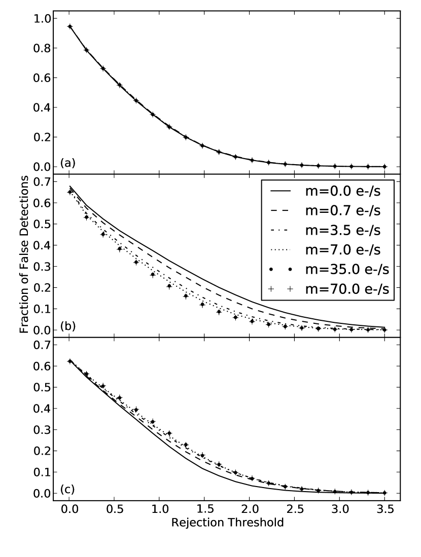
Figure 6.— Fraction of false detections versus rejection threshold is plotted here for various input slopes. (a) 2pt diff method. (b)dev from fit method. (c) y-int method.

The rejection threshold for different number of samples in a ramp is shown in Figure 7. An input slope of 70.0 $e^{-}$/s was used, and the rejection threshold was chosen such that the fraction of false detections was 0.05. The slope of these lines is 0.0011, 0.0065, and -0.0049 for the 2pt diff, dev from fit, and y-int methods respectively. Although this is a small change for the 2pt diff method, if a CR is found in a ramp then the rejection threshold was changed depending on the number of samples in a semi-ramp. If the rejection threshold was not calculated for a specific number of samples, we interpolated it. Figure 7 also shows how well the uncertainties in the 2pt diff method behave like a Gaussian, thus allowing the rejection threshold to be chosen easily.

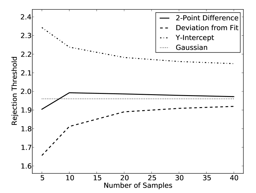
Figure 7.— Rejection threshold that will result in a fraction of false detections of 0.05 is shown for various sample numbers. What we would expect from a Gaussian distribution is also plotted to show how similar it is to the 2pt diff method. A slope of 70.0 $e^{-}$/s was used for this figure.

5.2. Slope and CR Detection

As we change the input slope of these ramps, we move from the read-noise-dominated regime to the photon-noise-dominated regime. In Figure 8 we show the two extremes: read-noise-dominated regime with an input slope of 0 $e^{-}$/s (Figure 8 (b) and (d)), and photon-noise-dominated regime with an input slope of 70 $e^{-}$/s (Figure 8 (a) and (c)). Plotted is the fraction of CRs found versus the CR magnitude and the fraction of false detections versus the CR magnitude.

In the photon-noise-dominated regime, photon-noise can appear as a CR as it is correlated and thus can lead to false detections. From Figure 8 (a) and (c) we see that all of the methods give similar results. However, note how the fraction of false detections for the 2pt diff method is relatively constant compared with the other two methods. This shows how well we are able to understand the uncertainties of this method. This, coupled with the fact that the 2pt diff method requires the least computations, leads us to suggest that the 2pt diff method is the optimal CR detection method in the photon-noise-dominated regime.

In the read-noise-dominated regime we only have random noise, and therefore we are able to get a more accurate calculation of the y-intercept and the y-intercept uncertainties. Therefore, as is shown in Figure 8 (b) and (d), in the read-noise-dominated regime the y-int method gives the best results in that it is able to find fainter CRs than the other two methods.

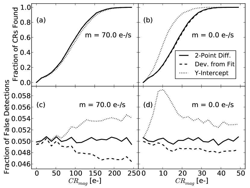
Figure 8.— CR detection rate and false detection rate as a function of CR magnitude for all three methods. In (a) and (c) the input slope was 70 $e^{-}$/s, in the photon-noise-dominated regime, where we recommend the 2pt diff method be used. In (b) and (d) the input slope was 0 $e^{-}$/s, in the read-noise-dominated regime, where the y-int method outperformed the other two. Each ramp has 40 samples.

In Figure 8 (d), note that the rate of false detections per CR strength is only constant for the 2pt diff method, while for the y-int method it is constant only for high-energy CRs. Between a $CR_{mag}$ of 0 $e^{-}$ and 10 $e^{-}$, we see a high fraction of false detections for the y-int method. This corresponds to the range where the CRs are not always found. The cause of this ’bump’ is not clear, and is evidence that we do not fully understand the noise model associated with the Y-INT method.

This could be caused by the fact that we treat each semiramp independently, which is inaccurate, since the uncertainties are correlated. Therefore, one solution could be to fit all semiramps simultaneously. This would increase the uncertainty, which would mean that the rejection threshold has been set too low (which would agree with what we see in the plots). We leave that for future work.

Regarding Figure 8 (a) and (b), if you draw a vertical line at a given $CR_{mag}$ (we chose the $CR_{mag}$ where the fraction of CRs found by the 2pt diff method is closest to 50%), you can see the difference between the fraction of CRs found by each method at that slope. We did this for slopes of 0.0$e^{-}$/s, 0.7$e^{-}$/s, 3.5$e^{-}$/s, 7.0$e^{-}$/s, 35.0$e^{-}$/s, and 70.0$e^{-}$/s. The results are shown in Figure 9. Each ramp had 40 samples, and again the rejection threshold was chosen such that the fraction of false detections was 5%. For comparison, we subtracted the fraction of CRs found by the 2pt diff method. In this figure we can see that we move into the regime where the y-int method performs better than the 2pt diff and dev from fit methods at a slope of $\sim 5e^{-}$/s.

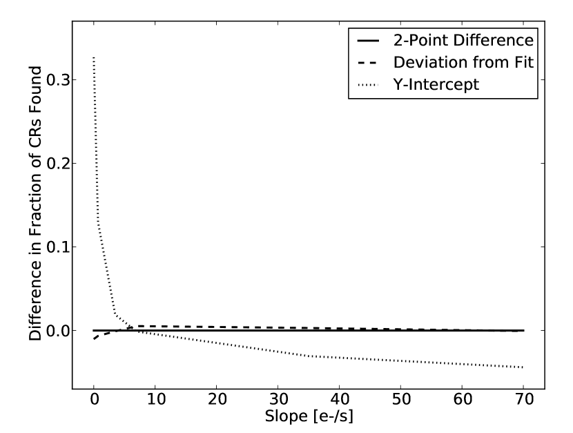
Figure 9.— Difference between the fraction of CRs found by the dev from fit and y-int methods to the 2pt diff method. From this plot we are able to see that the y-int method outperforms the other two with slopes less than $\sim 5e^{-}$/s.

To further illustrate how the results of each method change with input slope, we show the fraction of CRs found as a function of CR magnitude for different slopes and for each of our methods in Figure 10. The results of the 2pt diff and dev from fit methods appear to be similar, while the y-int method does better with lower slopes (read-noise-dominated regime).

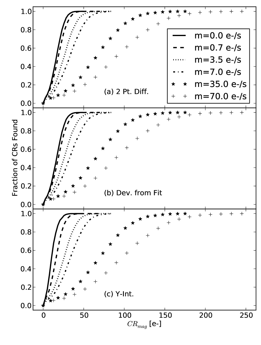
Figure 10.— CR detection rate as a function of CR magnitude for all methods. Each line is for a different input slope. There are 40 samples in each ramp.

5.3. Number of Samples and CR Detection

In order to determine how the number of samples in a ramp affects how well we detect CRs, we tested each algorithm on simulated ramps with 5, 10, 20, 30, and 40 samples. Figure 11 shows the fraction of CRs found as a function of CR magnitude for different numbers of samples for the 2pt diff, dev from fit, and y-int methods.

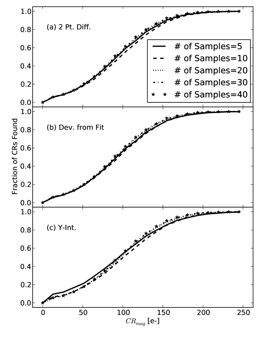
Figure 11.— CR detection rate as a function of CR magnitude for all methods. Each line is for a different number of samples in a ramp. The input slope is 70 $e^{-}$/s for each ramp.

When we use the 2pt diff method on weak CRs ($<$ 50 e^-) and strong CRs ($>$ 150 e^-), the fraction of CRs found increases with the number of samples (except for the case where there are five samples). For the dev from fit method, the fraction of CRs found increases with number of samples for string CRs, but shows no difference for weak CRs. Finally, for the y-int method, the fraction of CRs found decreases with number of samples for weak CRs, but increases with number of samples for strong CRs.

5.4. CR Sample Number and CR Detection

There are two questions when it comes to CR sample number: the first is where do we find false detections in the ramp, and the second is how well we find CRs in given positions in the ramp.

To answer the first question, we created a histogram of the sample numbers of the false detections found on simulated CR-free ramps for each method. These are presented in Figure 12. The results show that both the 2pt diff and dev from fit methods are not biased toward any position in the ramp. However, the y-int method is biased toward the last samples in a ramp where there is less effect from the correlation between samples.

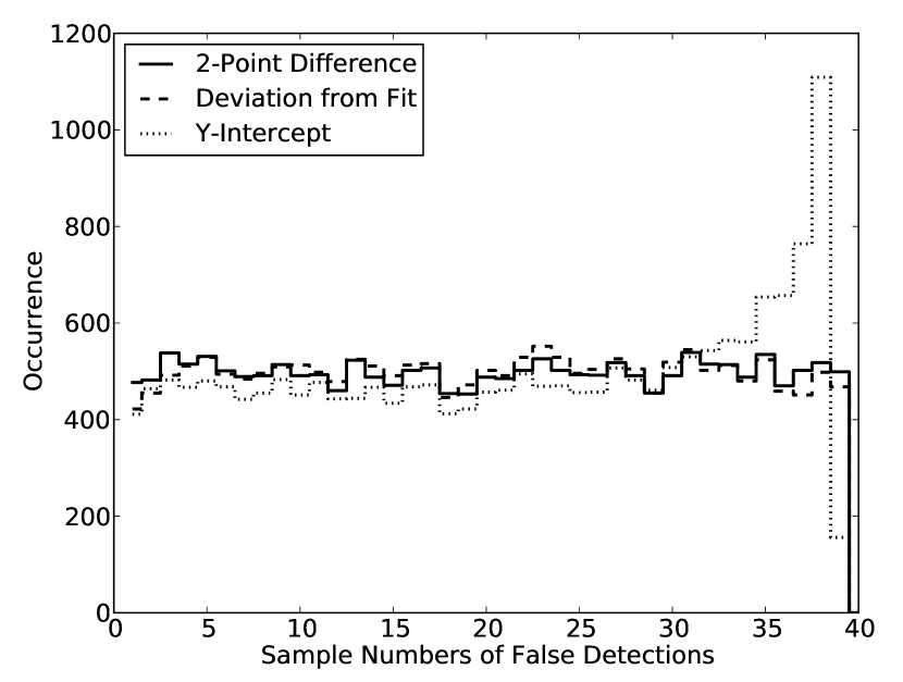
Figure 12.— Histograms of the sample numbers of the false detections for each method. These are from ramps without a simulated CR.

To answer the second question, we simulated ramps with 40 samples and input slope of 70 $e^{-}$/s, with one CR each at sample (numbers 3, 10, 20, 30, or 35). We then applied each of the algorithms to these ramps and compared the results, shown in Figure 13.

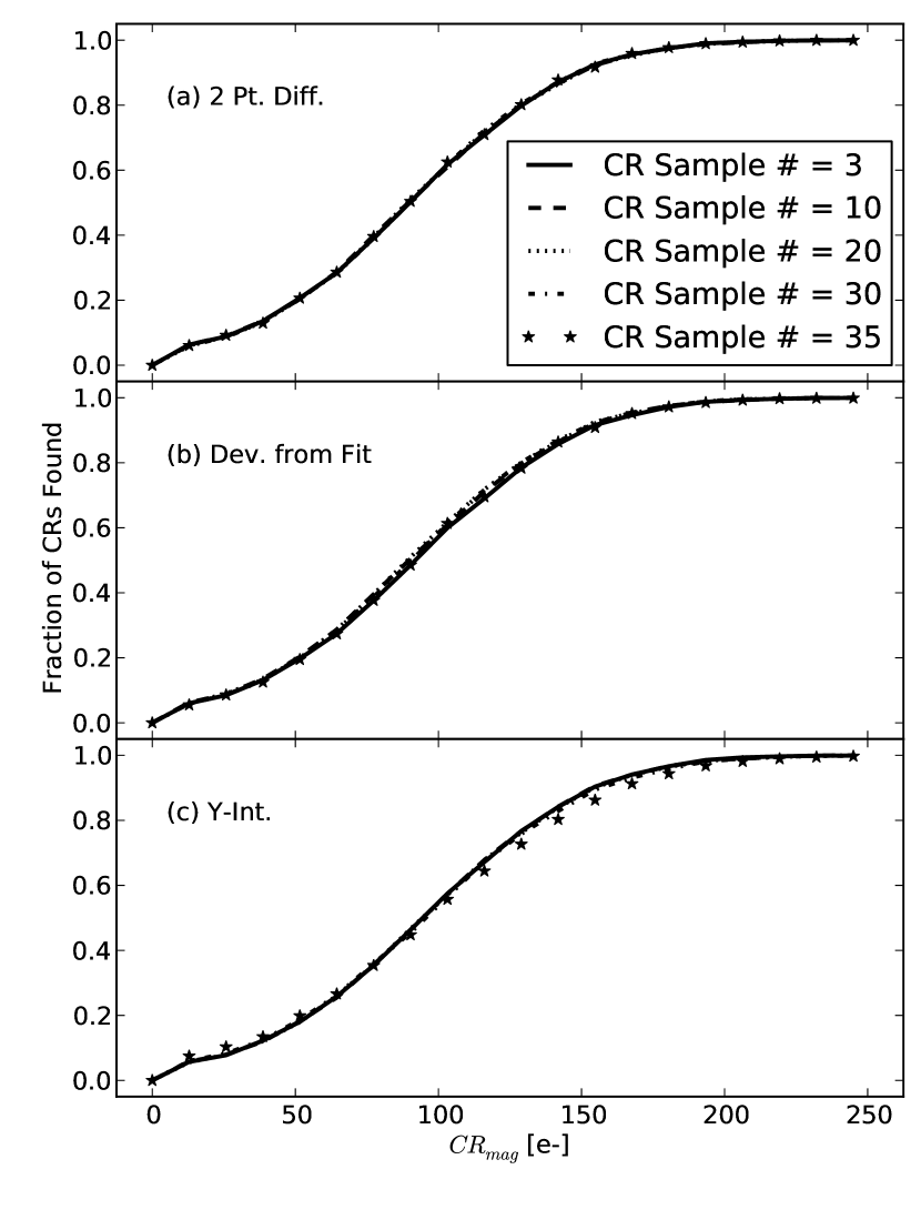
Figure 13.— CR detection rate as a function of CR magnitude for all methods. Each line is for a different CR sample number. The input slope is 70 $e^{-}$/s, and there are 40 samples in each ramp. The 2pt diff method is the only one to not show a dependence on sample number.

The results of these plots all show that the 2pt diff is the only method that does not vary depending on the sample number of the CR, as can be expected. Both the dev from fit and y-int methods are weakly biased by sample number. This is also expected, since both require fitting lines to data, and the fewer points in a line the less accurate the fit. Again, in the photon-noise-dominated regime, the 2pt diff method is best.

5.5. Multiple Cosmic Rays and CR Detection

In a 1000 s integration, if we assume that 20% of the field will be affected by CRs, then about 4% of the field could be affected by two CRs, and 0.8% could be affected by three. This is substantial enough that we need to account for this possibility.

To test how well each method does at handling multiple CRs, we simulated 10,000 40-sample ramps for each of 0-19 CRs. Each CR was of the same strength and in random but different samples. We show the results for 0-3 CRs in Figure 14.

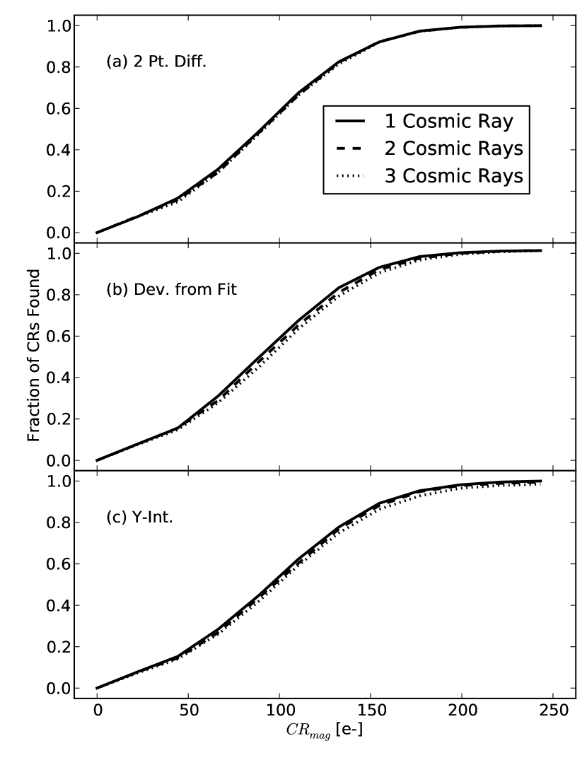
Figure 14.— CR detection rate as a function of CR magnitude. Each line is for a different number of CRs in a ramp.

As can be seen, the 2pt diff method shows no difference between one, two, or three CRs. We show only up to three CRs for simplicity, but we have found that the 2pt diff method does not start to show a difference in results until about nine CRs and therefore should be the optimal method in the photon-noise-dominated regime. Both the dev from fit and y-int methods, although show more variance than the 2pt diff method. This is caused by the fact that both methods require linear fits that will include two CRs for the y-int method (when assuming the correct location of one of the CRs), and all three CRs for the dev from fit method. Furthermore, for both methods the ramp will be segmented after the detection of the first CR.

6. Discussion

The three CR detection methods presented in this article were tested on simulated ramps, adjusted, corrected, and refined, in order to present optimum versions. We now compare our methods to determine which is best suited for various data.

6.1. 2-Point Difference Method

Our results show that the 2pt diff method performs best in the photon-noise-dominated regime. On top of being straightforward and computationally simple, we showed that the fraction of false detections versus rejection threshold is consistent regardless of slope and number of samples. We also showed that the uncertainties of the 2pt diff method follow a Gaussian distribution. Any deviation from a Gaussian was initially thought to be caused by the use of the median instead of average in the rejection criterion. However we found that while using the average did produce a more Gaussian shape, it was still not a perfect Gaussian. It was demonstrated that, as expected, the fraction of CRs found changed with slope and number of samples (though barely). Furthermore, we showed that the false detections are evenly distributed in all samples, and that the CR sample number did not change the results. Finally, we found that there is no noticeable difference in the performance of the 2pt diff method with multiple CRs, up to  9 CRs on a ramp with 40 samples.

Overall, the 2pt diff method is fast, consistent, and easy to understand and calibrate (e.g., choose a rejection threshold), and it gives the best results in the photon-noise-dominated regime.

6.2. Y-Intercept Method

For the y-int method, there are two regimes:

1. Photon-noise-dominated: In this regime the y-int method gives the same answer as the 2pt diff method. This is due to the correlated behavior of the noise in the ramps (e.g., a $3\sigma$ event due to the noise of the photons that have arrived in the last sample time will propagate through all subsequent samples, having the same effect as a CR). Calculating the linear fit of subsequent samples will not negate the fact that the noise in the photon-dominated regime is set by the noise in a single sample.

2. Read noise-dominated: In this regime the y-int method is better than the 2pt diff method. These two methods will still give the same results on any noise above the 2pt diff threshold, but anything below that will only be detectable by the y-int method. With the noise independent from sample to sample, a linear fit reduces the uncertainty in the y-intercepts and weaker CRs are detectable.

While it is unlikely that the uncertainty will be read-noise-dominated for most MIRI data (given the telescope and sky background), it will be the case for the JWST NIRSpec, NIRCam, and the Tunable Filter Imager (TFI). NIRSpec has a higher resolution than the TFI and therefore a lower background. Regardless, the TFI will likely be read-noise limited, given that it uses a tunable filter (narrowbands are less sky/telescope-dominated).

The y-int method, however, does not quite match the robustness of the 2pt diff method. In theory, these two methods should be the same in the photon-noise-dominated regime. However, the 2pt diff method gave more consistent results for different slopes, number of samples, and CR location in the ramps and for multiple CRs. The difference is that the 2pt diff method has a simpler noise behavior, while we have not fully solved for the noise behavior for the y-int method. Despite being careful when dealing with correlated and uncorrelated errors when fitting a line to a ramp or semiramp, we did not take this into consideration when taking the average of the slopes of the semiramps. Instead we use a weighted average, where the weights are simply the uncertainties in the slope. A solution to this problem would be to fit each semiramp and the CR simultaneously, as done by Robberto (2008) for uncorrelated errors only, modifying the method to account for correlated errors. Regardless, when working in the read-noise-dominated regime, the y-int method should be used.

6.3. Deviation from Fit Method

The dev from fit method did not perform as well as the other two methods. The y-int method dominated in the read-noise regime, and in the photon-noise-dominated regime the dev from fit method, like the y-int method, was not as consistent as the 2pt diff method when it came to different slopes, number of samples, CR location in the ramps, and multiple CRs. Therefore, to have a consistent fraction of false detections, we would have to set a new rejection threshold based on these variables. Furthermore, while not as complex at the y-int method, the dev from fit method is still more complex than the 2pt diff method and thus computationally more expensive. Finally, the uncertainties are nowhere near Gaussian, thus making it difficult to set the rejection threshold. The dev from fit method was only slightly worse at detecting CRs than the 2pt diff method, but given the fact that it is not as robust, and requires more CPU time, the dev from fit method is not recommended.

The dev from fit method could be improved by changing the weighting scheme so that instead of using the slope in the calculation of the photon-noise (since the slope will still include the CR in its calculation), we could use the median of the two-point differences as we do for the 2pt diff method. However, it still would not compare with the 2pt diff method, as we cannot do better than two$n_{r}$ terms and one $n_{p}$ term by the nature of our problem. Furthermore, even if we were able to get the same results for these two methods, the dev from fit method still requires larger computational resources than the 2pt diff method.

7. Conclusions

In this article we discussed three CR detection methods for nondestructive read ramps, as well as their strengths and weaknesses. We applied these methods to simulated ramps with single-sample groups. We showed that the covariance matrix must include correlated errors in order to improve the calculation of the slope and y-intercept of a ramp and their uncertainties. The y-int method benefits most from this use of the covariance matrix, and would not be an improvement of the 2pt diff method otherwise.

The 2pt diff method was shown to be able to give the best results in the photon-noise-dominated regime. The method’s uncertainties are quasi-Gaussian which simplifies the process of choosing a rejection threshold. Moreover, it is fast and consistent. Its robustness, compared with the other two methods, resides in the fact that we simply remove the two-point difference that includes the CR, instead of splitting the ramp into two semiramps, when searching for other CRs and calculating the slope and the y-intercept.

The dev from fit method results in a similar fraction of CRs found as the 2pt diff method for some ramps, but unlike the 2pt diff method these results change based on slope, number of samples, and CR location in the ramp and for multiple CRs. If we also consider the fact that it is computationally more expensive, we do not recommend this method for use in any regime.

The y-int method achieves the best results in the read-noise-dominated regime, and returns the same results as the 2pt diff method in photon-noise-dominated regime. In the photon-noise-dominated regime, the y-int method behaves like the 2pt diff method in that it is effectively calculating an average slope, excluding disturbances from any CRs (in the diff method this is done by taking the median of the two-point differences). The average slope is then divided by the noise due to one sample time: one photon-noise and two read-noise. The y-int method is better in the read-noise-dominated regime as the uncertainties on the line fit parameters diminish in size as more points are fit. This is not the case in the photon-noise-dominated regime due to the correlated nature of the noise. The y-int method only has two drawbacks: the noise model is not fully understood, and it is a complex algorithm.

In summary, if we take all results into consideration we are led to suggest that if only one method can be used on data cubes, the y-int method should be it. If computational speed is an issue then the 2pt diff method should be used, especially where photon-noise dominates, and the y-int method should only be used when the estimated slope is in the read-noise-dominated regime or where there is information, such as a nearby CR and cross-talk is suspected, to look for fainter effects.

8. Acknowledgments

This work was supported by the Space Telescope Science Institute, which is operated by AURA, Inc., under NASA Contract No. NAS5-26555.

We thank Howard Bushouse for providing the information on the method used by NICMOS and WFC3, which was called the dev from fit method here.

Appreciation goes to Harry Ferguson, David Grumm, Derck Massa, Mike Regan, and Massimo Robberto for their comments.

References

- Dahlen et al. (2008) Dahlen, T., et al. 2008, “Improvements to Calnica”, Instrument Science Report NICMOS 2008-002, (Baltimore: STScI)
- Dressel (2010) Dressel, L. 2010, “Wide Field Camera 3 Instrument Handbook”,Version 3.0, (Baltimore: STScI)
- Fixsen et al. (2000) Fixsen, D. J., Offenberg, J. D., Hanisch, R. J., Mather, J. C., Nieto-Santisteban, M. A., Sengupta, R., & Stockman, H. S. 2000, PASP, 112, 1350
- Gordon et al. (2005) Gordon, K. D., et al. 2005, PASP, 117, 503
- Hogg et al. (2010) Hogg, D. W., Bovy, J., & Lang, D. 2010, ArXiv e-prints
- Offenberg et al. (1999) Offenberg, J. D., Sengupta, R., Fixsen, D. J., Stockman, P., Nieto-Santisteban, M., Stallcup, S., Hanisch, R., & Mather, J. C. 1999, in Astronomical Society of the Pacific Conference Series, Vol. 172, Astronomical Data Analysis Software and Systems VIII, ed. D. M. Mehringer, R. L. Plante, & D. A. Roberts, 141–+
- Offenberg et al. (2001) Offenberg, J. D., et al. 2001, PASP, 113, 240
- Press et al. (1986) Press, W. H., Flannery, B. P., Teukolsky, S. A., & Vetterling, W. T. 1986, Numerical recipes. The art of scientific computing, ed. Press, W. H., Flannery, B. P., & Teukolsky, S. A.
- Rauscher et al. (2007) Rauscher, B. J., et al. 2007, PASP, 119, 768
- Robberto (2008) Robberto, M. 2008, JWST-STSCI-0001490, SM-12
- Robberto (2009a) —. 2009a, JWST-STScI-001928, SM-12
- Robberto (2009b) —. 2009b, JWST-STScI-001853, SM-12
- Robberto (2009c) —. 2009c, JWST-STScI-001928, SM-12
- Viana and Wiklind et al. (2009) Viana, A. and Wiklind, H. et al. 2009, “NICMOS Instrument Handbook”, Version 11.0, (Baltimore: STScI)
- Windhorst et al. (1994) Windhorst, R. A., Franklin, B. E., & Neuschaefer, L. W. 1994, PASP, 106, 798