Searching for Signatures of Cosmic String Wakes in 21cm Redshift Surveys using Minkowski Functionals

Abstract

Minkowski Functionals are a powerful tool for analyzing large scale structure, in particular if the distribution of matter is highly non-Gaussian, as it is in models in which cosmic strings contribute to structure formation. Here we apply Minkowski functionals to 21cm maps which arise if structure is seeded by a scaling distribution of cosmic strings embeddded in background fluctuations, and then test for the statistical significance of the cosmic string signals using the Fisher combined probability test. We find that this method allows for detection of cosmic strings with $G\mu>5\times 10^{-8}$, which would be improvement over current limits by a factor of about $3$.

I Introduction

The interest in searching for the signatures of cosmic strings in cosmological observations has been increasing. This is due in part to the realization that cosmic strings can arise in a variety of cosmological contexts. For example, in many inflationary models (both supergravity-based Rachel and string-based Tye ) the period of inflation ends with the formation of a network of cosmic strings. Such strings may also be produced in conventional phase transitions which occur after inflationary reheating . If they are topologically stable, the network of cosmic strings will persist at all times and will approach a ‘scaling solution’ characterized by a string distribution which is statistically independent of time if lengths are scaled to the Hubble radius (see e.g. ShelVil ; HK ; RHBrev for reviews of cosmic strings and their consequences for cosmology).

Cosmic strings are linear topological defects which arise in a wide range of quantum field theories as a consequence of a symmetry breaking phase transition. They are lines of trapped energy density and tension which is equal in magnitude to the energy density. They are analogous to defect lines in crystals or to vortex lines in superconductors and superfluids, except for the fact that the cosmic strings arise in relativistic field theories and hence obey relativistic dynamical equations of motion as opposed to the strings in condensed matter systems whose dynamics is typically friction-dominated. The trapped energy density associated with the strings leads to consequences in cosmology which result in clear observational signatures. Since the energy density per unit string length increases as $\eta^{2}$ as the symmetry breaking scale $\eta$ increases, cosmology provides the ideal venue to search for strings at very high energy scales. Thus, searching for strings in cosmological observations provides an avenue complementary to accelerator experiments for looking for signals of physics beyond the Standard Model: accelerator signals are more easily seen for low symmetry breaking scales, while signals in cosmology are more easily detected for larger values of $\eta$.

Because of the scaling solution of the cosmic string network, cosmic strings lead to a scale-invariant spectrum of cosmological perturbations, as in inflationary models (see e.g. CSearly ). However, the string-induced density fluctuations are highly non-Gaussian, an effect which is eliminated when computing the usual power spectrum of density fluctuations. It follows that string signals are much easier to detect in position space than in momentum space.

The scaling network contains two types of strings, a network of ‘infinite’ strings and a distribution of string loops with radii smaller than the Hubble radius. String loops oscillate because of their relativistic tension and slowly decay by emitting gravitational radiation. Their gravitational effects are similar to those of a point mass CSearly . In this paper we are interested in the characteristic non-Gaussian effects of long string segments and will not further consider cosmic string loops (which produce 21cm signals which are harder to differentiate from noise Pagano ).

Due to the relativistic tension of the strings, an infinite string segment will typically have a velocity in the plane perpendicular to the string which is of the order of the speed of light . Since space perpendicular to a long straight string is conical with a ‘deficit angle’ given by deficit

$$\alpha\,=\,8\pi G\mu\,,$$ (1)

where $G$ is Newton’s constant and $\mu$ is the mass per unit length of the string (which is proportional to $\eta^{2}$) , a string moving with velocity $v_{s}$ through the matter gas of the early universe at some time $t_{i}$ will lead to a ‘wake’ wake , a thin wedge behind the string with twice the background density whose planar dimensions are

$$c_{1}t_{i}\times v_{s}\gamma_{s}t_{i}\,.$$ (2)

Here, $\gamma_{s}$ is the relativistic $\gamma$ factor associated with the velocity $v_{s}$, and $c_{1}$ is a constant of order one which is proportional to the curvature radius of the long string network in units of the Hubble radius. The mean thickness $h$ of the wake is initially

$$h\,=\,4\pi G\mu v_{s}\gamma_{s}t_{i}$$ (3)

and for $t>t_{i}$ it increases by gravitationally accreting matter from above and below the wake wakegrowth .

Current observations (in particular the oscillatory features in the angular power spectrum of cosmic microwave background (CMB) anisotropies) set an upper bound on the string tension of the order $G\mu<1.7\times 10^{-7}$ Dvorkin ; CSbound , which corresponds to cosmic strings contributing less than $5\%$ to the total spectrum of inhomogeneities. We will discuss this in more detail in section II. In this paper, we are therefore considering a setup in which there is a contribution of cosmic strings to the power spectrum in addition to the dominant component of Gaussian, nearly scale-invariant fluctuations (such as can be produced in inflationary cosmology Guth ; Mukh or in string gas cosmology SGC ).

Cosmic string wakes give rise to distinctive signatures in the large-scale distribution of matter in the universe. As discussed in LSS , they lead to planar structures in the distribution of galaxies. Since wakes present between the time of last scattering of the CMB and today represent overdense regions of electrons, they lead to extra scattering of CMB photons and hence to distinctive rectangular regions in the sky with extra CMB polarization Danos1 (with statistically equal B-mode and E-mode components). The effect relevant to the current paper is that wakes represent overdense regions of neutral hydrogen and hence Danos2 lead to wedge-like regions in 21cm redshift surveys of extra 21cm absorption or emission . The amplitude of the position space signal is independent of the string tension $\mu$ and can be as large as $100{\rm mK}$ . The width of the wedge, however, depends linearly on $\mu$. A crucial point is that wakes exist as non-linear structures at high redshifts since as soon as the string passes by, a wake with overdensity 2 forms. This is to be contrasted to the situation in Gaussian models with a scale-invariant spectrum of primordial cosmological perturbations in which no nonlinear structures exist until quite low redshifts. In particular, at redshifts larger than that of reionization, the cosmic string signal should stand out against the effects of Gaussian fluctuations and noise. Thus, 21cm redshift surveys appear to be an ideal window to search for cosmic string signals.

If cosmic strings exist, then the induced 21cm maps will not only contain the characteristic wedges of extra absorption or emission. They will also contain noise, most importantly Gaussian noise from the primordial Gaussian density fluctuations which must be present in addition to the string-induced perturbations. Good statistical tools will be required in order to extract the string signals in a quantitative and reliable way.

In this report we study the possibility that Minkowski Functionals Hadwiger , a tool for characterizing structure which is orthogonal to the usual way of characterizing maps using correlation functions, can be applied to identify cosmic string signals in 21cm redshift surveys at reshifts larger than that of reionization. The theory behind Minkowski Functionals has its roots in Integral Geometry and Hadwiger’s Theorem, which states that a $d$-dimensional set of convex bodies can be completely described by $d+1$ functionals. Minkowski functionals have been applied numerous times in cosmology, e.g. to the distribution of galaxies on large scales superclusters and the analysis of CMB maps CMB . There have also been attempts to apply Minkowski functionals to search for signatures of cosmic strings in the large-scale structure of the distribution of galaxies CSMink . Since for 21cm redshift surveys the contributions to the ‘noise’ from the Gaussian source of primordial fluctuations is in the linear regime at the high redshifts we are interested in (larger than the redshift of reionization), we expect that Minkowski functionals will be very powerful in extracting cosmic string signals in the case of 21cm maps.

The outline of this paper is as follows: in the following section we outline current observational limits on cosmic strings as well as prospects for future detection. In Section III we briefly review the toy model for the cosmic string scaling distribution which we use and describe the theoretical 21cm maps induced by cosmic strings. Section IV then repeats the methodology of section III but including a simulation of the background noise. In Section V we review the theory and calculation of Minkowski functionals, before presenting our results in Section VI. We conclude with a summary of our results and a discussion of future work.

II Observational Constraints

The strongest constraints on cosmic strings currently come from measurements of the angular power spectrum of the cosmic microwave background (CMB). The WMAP data provided no hints of cosmic strings, and hence placed an upper bound on the string tension CSbound . Specifically, it constrained the string contribution to the primordial power spectrum to be less than 10%. However, there are now CMB experiments with better angular resolution than WMAP provided and which can yield improved bounds on the cosmic string tension. The Atacama Cosmology Telescope (ACT) ACT , a six-meter off-axis telescope with arcminute-scale resolution located in the Atacama desert in northern Chile, and the South Pole Telescope (SPT) SPT , a 10 meter telescope located in Antarctica which can study the small-scale angular power spectrum of the CMB, both are providing excellent data. A recent analysis of the angular power spectrum of CMB anisotropies from joint SPT and WMAP7 Dvorkin made use of a Markov Chain Monte Carlo likelihood analysis to place a limit on the string tension of $G\mu<1.7\times 10^{-7}$ (at 95% confidence). This analysis was done in the context of the zero width cosmic string toy model which we will also use in the following. A similar limit was found by CMBandACT , who used combined WMAP7, QUAD and ACT data to place limits on the tension of Abelian Higgs model strings. The resulting bound on the string tension was $G\mu<4.2\times 10^{-7}$.

The difference in the results is mostly due to the uncertainties in the distribution of strings. Due to the very large range of scales involved (the width of a cosmic string is microscopic but the length is cosmological), numerical simulations of both field theory and Nambu-Goto strings involve ad hoc assumptions and/or extrapolations. The uncertainties in the resulting string distributions appear in free parameters (e.g. the number of long string segments per Hubble volume and the value of the constant $c_{1}$) of toy models distributions of cosmic strings. These uncertainties effect the angular power spectrum of CMB anisotropies.

Local position space searches for signals of individual cosmic strings are less sensitive to the uncertainties in the string distribution than power spectra. This is the idea behind the proposal of Amsel ; Stewart ; Danos0 to search in position space for the line discontinuities in CMB anisotropy maps which long straight cosmic strings produce due to the Kaiser-Stebbins KS effect. It was proposed to analyze position space anisotropy maps using of the Canny edge detection algorithm. It was shown Danos0 that strings with $G\mu\geq 10^{-8}$ might be detectable with this method. Application of this method to the SPT or ACT data may yield interesting results

Another avenue for detection of cosmic strings is via gravitational waves, which will be produced by oscillating cosmic strings and/or the decay of cosmic string loops. Cosmic strings in fact CSGR produce a scale-invariant spectrum of gravitational waves with an amplitude which is similar to or larger than the amplitude of gravitational waves from simple inflationary models. Pulsar timing pulsar or direct detection (e.g. making use of the Laser Interferometer Gravitational-Wave Observatory (LIGO) Abbott:2007kv ) provide means for searching for the cosmic string signal. However, at the moment the bounds are not competitive with bounds obtained from the CMB .

We are currently entering a revolution in radio astronomy, with both the Square Kilometer Array (SKA) SKA and the European Extremely Large Telescope (E-ELT)E-ELT aiming to be operational by early 2020. Of particular interest (in terms of potential to observe cosmic strings) is the SKA, which as the name implies will consist of 1 million square meters of collecting area. There are many ongoing projects to develop the science and technology necessary to operate the SKA. These are categorized into: (1) Precursor Facilities, which will physically be at the SKA site carrying out SKA-related projects, (2) Pathfinder Experiments, which will develop SKA-related science and technology off-site, and (3) Design Studies, which will investigate technologies and develop prototypes. Many of these projects are world class facilities in there own right, and we will mention some of the experiments which may have a chance of observing cosmic strings.

One such project is LOFAR lofar , a Pathfinder experiment, which is measuring the neutral hydrogen fraction of the inter-galactic medium. This will map out the epoch of reionization between redshifts 11.5 and 6.7, and will be capable out of arc-minute resolution. For 21cm measurements, the redshift range of LOFAR extends to the “Dark Ages” before reionization, redshifts where the cosmic string signal will be cleanest. Another SKA project with potential to observe cosmic strings is the MEERKAT experiment Holwerda:2011kd , which is carrying out a project titled MESMER that will track the neutral hydrogen content of the early universe by using carbon monoxide as a proxy. To make an accurate prediction as to the clumping of carbon monoxide around a cosmic string would require semi-analytical hydrodynamics calculations, but to a rough approximation we should expect to see the characteristic wedge of emission/absorption.

III The Cosmic String Signal

III.1 Modelling the signal

In any theory which leads to the formation of stable cosmic strings in the early universe, a network of strings will persist at all later times, and this network will approach a ‘scaling solution’, meaning that the statistical properties of the network of cosmic strings are independent of time if all distances are scaled to the Hubble radius. The existence of the scaling solution can be argued for using analytical arguments (see e.g. ShelVil ; HK ; RHBrev ), and it has been confirmed using extensive numerical simulations CSnum .

The scaling distribution of strings consists of a network of long strings of mean curvature radius $\zeta=c_{1}t$ (where $c_{1}$ is a constant of order 1), and string loops with a much smaller radius that result from intersection and hence ‘cutting’ of the long strings. As a consequence of their relativistic tension, the long strings have typical translational velocities $v_{s}$ close to the speed of light. Hence, Hubble length string segments will intersect with other such segments with probability close to one on a Hubble time scale. By this process, string loops are formed and the correlation length of the long string network (the mean curvature radius) increases in comoving coordianates to keep up with the Hubble radius, as confirmed in the numerical string evolution simulations CSnum .

As is commonly done in studies of the cosmological consequences of cosmic strings, we use an analytical toy model of the infinite string network which was first introduced in Periv : we divide the time interval of interest (usually the time between the time $t_{eq}$ of equal matter and radiation and the present time $t_{0}$) into Hubble time steps. In each time step we lay down an integer number $N_{H}$ per Hubble volume of straight string segments of length $c_{1}t$ with random midpoints and random tangent vectors. The string segments in neighboring Hubble time steps are taken to be independent. The long strings are taken to have a velocity $v_{s}$ orthogonal to their tangent vectors. Each such string will produce a wake whose thickness grows in time.

We will be interested in signals which are emitted at a time $t_{e}>t_{i}$ from string wakes laid down at any time $t_{i}$ between $t_{eq}$ and the present time . Since the planar dimensions of the wake (whose initial physical dimensions are given in (2)) are constant in comoving coordinates, their physical size grows with the scale factor. The comoving thickness of the wake, whose initial physical length is given by (3), grows linearly with the scale factor because of gravitational accretion. Hence, the dimensions of the wake at $t_{e}$ in physical coordinates are given by:

$$\frac{z_{i}+1}{z_{e}+1}\bigl{[}c_{1}t_{i}\times t_{i}v_{s}\gamma_{s}\times 4\pi G\mu t_{i}v_{s}\gamma_{s}\frac{z_{i}+1}{z_{e}+1}\bigr{]}\,,$$ (4)

where $z_{e}$ is the emission redshift $z(t_{e})$.

The dominant form of the baryonic matter in the universe before reionization is neutral hydrogen (H), which we detect via the 21cm hyperfine line. Measuring the intensity of the redshifted 21cm radiation from the sky has the potential of giving us three dimensional maps of the distribution of neutral hydrogen in the universe (see e.g. Furl for an in-depth review article on 21cm cosmology). As explained in detail in Danos2 , since wakes are overdense regions of neutral hydrogen, they will lead to excess 21cm emission or absorption. We will see this excess in directions for which our past light cone intersects a wake at some time $t_{e}>t_{rec}$, $t_{rec}$ being the time of recombination. This 21cm signal has the special geometry given by the wake geometry - a thin wedge in the three-dimensional 21cm redshift survey (see Figure 1), and it is this special geometry which provides the ‘smoking gun’ signal for cosmic strings, the signal which we are trying to extract using Minkowski functionals in this report.

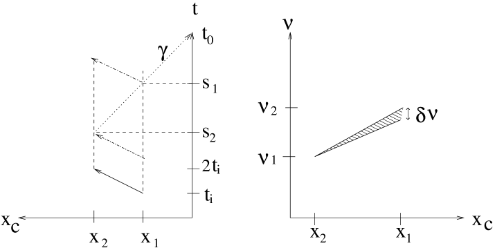
Figure 1: The right panel depicts a sketch of the string wake-induced wedge of extra emission/absorption in 21cm redshift surveys. The horizontal axis represents the two angular directions, the vertical axis redshift. The left panel is a space-time sketch showing the position of the string which gives rise to the wedge of the right panel. Here, the vertical axis is time, and the horizontal axis corresponds to comoving spatial coordinates. Note, in particular, the positions where the string wedge intersects the past light cone of an observer at the current time $t_{0}$. The almost horizontal lines represent the string at the time when it forms the wake ($t_{i}$), and the wedge at the times $s_{1}$ and $s_{2}$ when the back (and front) of the wake intersect our past light cone.

Since already at the initial time $t_{i}$ the wake is a non-linear density fluctuation, the matter being accreted onto the wake will collapse onto the wake, shock heat and thermalize . The hydrogen (H) atoms inside a wake laid down at redshift $z_{i}$ will have a temperature at time $t_{e}$ given by:Danos2

$$T_{K}(t_{e})\,=\,\frac{16\pi^{2}}{75}(G\mu)^{2}(v_{s}\gamma_{s})^{2}\frac{z_{i}+1}{z_{e}+1}\frac{m}{k_{B}}\,,$$ (5)

where $m$ is the proton mass. Inserting numerical values, and expressing $G\mu$ in units of $10^{-6}$ and so written as $(G\mu)_{6}$, we obtain

$$T_{K}(t_{e})\,\approx\,[20K](G\mu)^{2}_{6}(v_{s}\gamma_{s})^{2}\frac{z_{i}+1}{z_{e}+1}\,.$$ (6)

Note that the numerical simulations by sornborger show that the temperature can be taken to be approximately uniform inside of the wake.

The quantity of interest is the brightness temperature $T_{b}$ due to 21cm transitions of the Hydrogen in the wake, or more specifically the difference $\delta T_{b}$ in brightness temperature between photons from the wake and those from the surrounding space, From this point onwards, ‘brightness temperature’ will refer to $\delta T_{b}$, defined by

$$\delta T_{b}(z_{e})\,=\,\frac{T_{b}(z_{e})-T_{\gamma}(z_{e})}{1+z_{e}}\,,$$ (7)

where $T_{\gamma}(z_{e})$ is the redshifted CMB temperature, and $T_{b}(z_{e})$ is the brightness temperature due to 21 cm emission in the wake. A full derivation which can be found in Danos2 yields the following expression for $\delta T_{b}$:

$$\delta T_{b}(z_{e})\,=\,[0.07\textit{K}]\frac{x_{c}}{x_{c}+1}\left(1-\frac{T_{\gamma}}{T_{K}}\right)\sqrt{1+z_{e}}\,,$$ (8)

where several constants have been absorbed into the prefactor, which can be found in the original derivation by Danos2 . Note that the collision coefficient $x_{c}$ is given by Furl :

$$x_{c}\,=\,\frac{n\kappa_{10}^{HH}}{A_{10}}\frac{T_{\star}}{T_{\gamma}}\,,$$ (9)

where $T_{\star}$, taken to be 0.068 K, is the temperature corresponding to the hydrogen energy splitting $E_{10}$, $A_{10}$ is the spontaneous emission coefficient of the 21cm transition, $n$ is the number density of hydrogen atoms, and $\kappa_{10}^{HH}$ is the de-excitation cross section which is given in Furl . Using equation (8), the brightness temperature for a given wake with a given value of $z_{e}$ can be obtained, which in conjunction with the spatial dimensions of the wake, allows a 3-D map of brightness temperature to be generated.

III.2 Generating Temperature Maps

In the following we will outline the steps in the construction of 21cm redshift maps in the case of primordial perturbations produced exclusively by strings. We will consider hypothetical sky maps covering a patch of the sky of angular scale $\theta\times\theta$. First, we must compute the number of strings which contribute to the sky signal in this patch. This is the number of strings whose wakes at some point in time between $t_{rec}$ and $t_{0}$ intersect the observer’s past light cone with opening angle $\theta$.

III.2.1 Distribution of Strings

According to our model of the distribution of a scaling string network we divide the time between $t_{eq}$ and the present time $t_{0}$ into Hubble time steps. For each such time step centered at time $t_{i}$ we now compute the number $N(t_{i})$ of string wakes which at some point in the future of $t_{i}$ will intersect the past light cone corresponding to an observational angle $\theta$ (a box of size $\theta\times\theta$ on the sky).

We first note that $N(t_{i})$ is given by the ratio of the comoving volume of the past light cone

$$V_{p}(\theta)\,\simeq\,27\bigl{(}\frac{\theta}{2\pi}\bigr{)}^{2}t_{o}^{3}$$ (10)

divided by the comoving Hubble volume at time $t_{i}$

$$V_{H}(t_{i})\,=\,t_{i}t_{0}^{2}\,,$$ (11)

multiplied by the number $N_{H}$ of strings per Hubble volume in the scaling solution (a number which according to numerical simulations is in the range $1<N_{H}<10$ CSnum . This gives

$$N_{i}\,\simeq\,N_{H}27\bigl{(}\frac{\theta}{2\pi}\bigr{)}^{2}z(t_{i})^{3/2}\,.$$ (12)

Now that we know the total number of string wakes produced at redshift $z_{i}$ which will be seen in the simulation box, we need to determine the distribution of the redshift $z_{e}$ at which they will cross the past light cone of the simulation region in the sky. This can be determined by remembering that light travels in a straight line in conformal coordinates (comoving spatial coordinates and conformal time $\tau$). Hence, the number of wakes which intersect the past light cone at conformal time $\tau$ (where the conformal time is measured backwards, meaning $\tau=0$ at the present time and $\tau$ increases as we go back in time) in a conformal time interval $d\tau$ is

$$dN_{i}(\tau)\,=\,\bigl{(}\frac{\tau}{\tau_{eq}}\bigr{)}^{2}{\cal N}d\tau\,,$$ (13)

where ${\cal N}$ is determined by demanding that the integral over $\tau$ from $\tau_{i}\equiv\tau(t_{i})$ to $\tau(t_{0})$ gives $N_{i}$. The result can be integrated from $0$ to $\tau_{e}$ to yield the number of string wakes $N_{i}(\tau_{e})$ which intersect the past light cone at a time later or equal to $\tau_{e}$:

$$N_{i}(\tau_{e})\,=\,\left(\frac{\tau_{e}}{\tau_{i}}\right)^{3}N_{i}\,.$$ (14)

To determine the redshift distribution of emission times $z_{e}$, we need to relate the conformal time $\tau_{e}$ to the emission redshift $z_{e}$. We start by expressing $\tau_{e}$ in terms of $t_{e}$,

$$\mathrm{d}\tau_{e}=\frac{\mathrm{d}t_{e}}{a(t_{e})}\,,$$ (15)

which evaluates to

$$\tau_{e}=3t_{0}\left[1-\left(z_{e}+1\right)^{-\frac{1}{2}}\right]\,.$$ (16)

An expression for the number $N_{i}(z_{e})$ of string wakes with an emission redshift larger or equal to $z_{e}$ can now be obtained by substituting the preceding equation into equation 14, and using our expression for $N_{i}$ from 12. This gives

$$N_{i}(z_{e})\,=\,N_{H}27\bigl{(}\frac{\theta}{2\pi}\bigr{)}^{2}z(t_{i})^{3/2}\left[\frac{1-\left(z_{e}+1\right)^{-\frac{1}{2}}}{1-\left(z_{i}+1\right)^{-\frac{1}{2}}}\right]^{3}$$ (17)

Due to the discrete nature of this simulation, we need to approximate this relationship by splitting the redshift space into slices, and laying down strings in each slice. The smallest possible slice would be the number of discrete values of redshift in the simulation (128, as we will discuss shortly) divided by the range of redshift, which we shall take to be 50 for this example. However, as we must have an integer numbers of wakes, a slice this small would result in the majority of slices having 0 wakes. Hence we instead choose a slice thickness $\Delta z_{e}=1$, which will contain a number of wakes given by

$$\Delta N_{i}(z_{e},z_{e}-1)\,=\,\left[1.41\times 10^{6}\right]$$ (18)

$$\,\,\,\,\,\,\left[-2(x+1)^{-1/2}+2x^{-1}-\frac{2}{3}x^{-3/2}\right]_{z_{e}-1}^{z_{e}}\,,$$

where we have included all prefactors into the constant. A plot of this distribution is shown in Figure 2. As is apparent, the largest number of wakes intersect the past light cone at low redshifts. This can be understood since the low redshift range covers most of the physical volume.

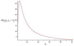
Figure 2: Distribution of the redshifts at which the string wakes intersect the past light cone (for a fixed time $z_{i}=10^{3}$ at which the strings were produced). The horizontal axis is the emission redshift $z_{e}$, the vertical axis is the number $\Delta N_{i}(z_{e},z_{e}-1)$ of string wakes produced at redshift $z_{i}$ (taken to be $10^{3}$) which intersect the past light cone of the sky area we are considering in the redshift interval between $z_{e}-1$ and $z_{e}$.

III.2.2 Angular and Redshift Scales of a Wake-Induced Wedge

As discussed in Section 2, each string wake which intersects the past light cone of the observer’s angular patch will lead to a thin wedge of extra 21cm absorption or emission. We are concerned with string wakes produced at time $t_{i}$ which intersect the past light cone of the observational patch at some time $t_{e}>t_{rec}$. Each such string wake will lead to a thin wedge in a 21cm redshift survey of a certain angular extent and certain thickness.

First, let us consider the angular extent of the wedge. A string laid down at a time $t_{i}$ will create a wake with physical dimensions given by equation 4. To calculate the angular size of a wake, one must start with the physical length of the wake at time $t_{i}$ which in direction tangent to the string is:

$$x_{p}(t_{i})\,=\,c_{1}t_{i}\,,$$ (19)

where (as we recall from before) $c_{1}$ is a constant of order 1. In the direction of string motion the size is the same except that the factor $c_{1}$ gets replaced by $v_{s}\gamma_{s}$. In our work we choose the rather realistic parameter values where the two constants are the same. The corresponding comoving distance is then given by

$$x_{c}(t_{i})\,=\,\left(\frac{t_{0}}{t_{i}}\right)^{\frac{2}{3}}x_{p}(t_{i})=(z_{i}+1)^{-1/2}c_{1}t_{0}\,.$$ (20)

Hence, the corresponding angle $\theta_{i}$ is:

$$\theta_{i}\,=\,(z_{i}+1)^{-1/2}c_{1}\times 90^{o}\,.$$ (21)

For the most numerous and thickest wakes, $z_{i}+1=1000$, and if the constant $c_{1}$ is taken to be $1/3$ , the answer is then approximated by:

$$\theta_{i}\,=\,(z_{i}+1)^{-1/2}\times 30^{o}\,$$ (22)

which yields approximately $1^{o}$ as the angle of the wake-induced wedge.

Since the string which produces the wake is moving, the string-induced wake is slightly “tilted” in the three-dimensional redshift-angle space, i.e. the tip of the wedge (which corresponds to the string at the latest time) is at a slightly larger redshift than the mean redshift of the tail of the wedge (where the string was at the initial time). This does not change the fact that the projection of the wedge onto the angular plane has the dimension given above. However, when computing the projection into the redshift direction we have to be careful. The wedge is thin in direction perpendicular to the plane of the wedge, but this perpendicular direction is at an angle relative to the redshift direction. In the following we will compute the thickness of the wedge in perpendicular direction to the wedge plane.

We now calculate the thickness of the wake in the perpendicular direction. The finite thickness in redshift direction originates from the fact that photons originating from different parts of the wake are redshifted by slightly different amounts. The starting point of the computation is the formula

$$z+1\,=\,\left(\frac{t}{t_{0}}\right)^{\frac{2}{3}}$$ (23)

valid in the matter-dominated period. Taking differentials, and setting $t=t_{e}$ yields

$$\Delta z\,=\,\left(\frac{2}{3}\right)t_{0}^{-2/3}t_{e}^{-1/3}\Delta t_{e}\,,$$ (24)

where $\Delta t_{e}$ is the time delay between photons from the top and the bottom of the wedge. We compute $\Delta t_{e}$ at the midpoint of the wake (point of medium thickness). This is given by the thickness of the wake, which, as discussed in Danos2 grows linearly in comoving coordinates because of gravitational accretion onto the initial overdense region.

Using linear perturbation theory, the width of the wake at time $t_{e}$ is

$$w(t_{e})\,=\,4\pi G\mu v_{s}\gamma_{s}t_{0}\bigl{(}z(t_{i})+1\bigr{)}^{1/2}\bigl{(}z(t_{2})+1\bigr{)}^{-2}\,,$$ (25)

which equals $\Delta t_{e}$. Hence, from (24) it follows that

$$\Delta z\,=\,\frac{8\pi}{3}G\mu v_{s}\gamma_{s}\bigl{(}z(t_{i})+1\bigr{)}^{1/2}\bigl{(}z(t_{2})+1\bigr{)}^{-3/2}\,.$$ (26)

The analysis of gravitational accretion performed using the Zel’dovich approximation instead of with naive linear cosmological perturbation theory yields the same result Danos2 except that the coefficient is $24\pi/5$ instead of $8\pi/3$.

Once the dimensions of the wake are calculated, it remains to map this onto a 3-D lattice of points from which the Minkowski Functionals can be calculated. To do this requires setting the resolution with which the wakes will be studied, and then scaling up the dimensions of the wake. For the purposes of this simulator, we use a lattice of side length $128$, and study a volume that subtends an angle of $10^{o}$ in both the angular directions, with $z_{e}$ ranging from 5 to 50, and $N_{H}=3$. In this case, the angular resolution is $10^{o}/128=.078^{o}$, while the resolution in the redshift direction is $45/128=.35$. To scale up the dimensions of the wake only requires multiplying each dimension by the inverse of the resolution (ie: $128/45=2.84$ in the $z_{e}$ direction).

III.2.3 Brightness Temperature: $\delta T_{b}$

The final step in the calculation is to determine the brightness temperature at every point of the three dimensional angle-redshift map $(\theta,\phi,z)$. Any point for which the past light ray in angular direction $(\theta,\phi)$ does not intersect a wake at redshift $z$ yields zero brightness temperature. A point which at redshift $z_{e}$ is intersecting a wake due to a string present at time $t_{i}$ is assigned a non-vanishing brightness temperature given by Equation (8), with $T_{K}$ obtained from Equation (6). Overlapping wakes are assumed to be non-interacting.

IV Background Noise

IV.1 Modelling the Signal

As discussed in the introductory section, in our setup the cosmic strings only make a contribution of less than $5\%$ to the total power spectrum of inhomogeneities. The dominant contribution is in the form of an approximately scale-invariant spectrum of Gaussian perturbations such as can be produced in a number of cosmological scenarios, e.g. in inflationary cosmology Mukh or in string gas cosmology SGC . The dominant Gaussian fluctuations are in the linear regime until late times on large length scales and are hence not expected to contribute a lot to 21cm fluctuations at high redshifts (redshifts before reionization). There will, however, be smaller scale fluctuations which become non-linear, forming so-called “mini-halos” which then contribute to the spectrum of 21cm fluctuations. It is crucial for us to check that the cosmic string effects can be detected above the noise from the Gaussian fluctuations (which we call “background noise” in the following).

The contribution of “background noise” to the 21cm fluctuations of the universe has been studied in detail (see e.g. shapiroAnalytical ; arXiv:1005.2502 ). As was shown, there is an effect on 21cm maps which comes from the diffuse inter-galactic medium (IGM). However, this effect is homogeneous in space on the cosmological scales which interest us here and will hence not be further considered in this paper. Instead, we focus on the contribution of the inhomogeneities mentioned above which lead to the formation of mini-halos. This contribution has been studied done both semi-analytically, shapiroAnalytical , and later using large scale numerical simulations arXiv:1005.2502 .

To calculate the signal from minihalos we must find the mass function $\mathrm{d}n/\mathrm{d}M$, which can, when integrated over a range of masses, give the number density for minihalos in this mass range. There are two possible mass profiles for minihalos, the Sheth-Tormen model and the Press-Schechter model. Recent numerical simulations support the Press-Schecter model, (see Figure 2 of arXiv:1005.2502 ). Once we know the mass function, the brightness temperature is then calculated using line of sight integrals given a realization of the inhomogeneities described by the mass function.

The Press-Schecter function for the number density of minihalos is given by Press:1973iz :

$$N(M)\mathrm{d}M=-\left(\frac{\bar{\rho}}{M}\right)\left(\frac{2}{\pi}\right)^{1/2}\frac{\delta_{c}}{\sigma^{2}}\frac{\mathrm{d}\sigma}{\mathrm{d}M}e^{-\frac{\delta^{2}_{c}}{2\sigma^{2}}}\mathrm{d}M$$ (27)

where $\bar{\rho}$ is the mean (baryonic and dark) matter density of the universe, and $\sigma^{2}(M,t)=\langle\delta^{2}_{M}\rangle(t)$ is the root mean square mass fluctuation on the mass scale $M$. Halos will form in regions with a $\delta_{M}$ above a critical fluctuation $\delta_{c}\approx 1.69$. Our number density simplifies to:

$$N(M,z)\mathrm{d}M = \Omega_{m}\left(\frac{(3+n)}{6}\right)\left(\frac{\bar{\rho}}{M^{2}}\right)$$

$$\times\left(\frac{2}{\pi}\right)^{1/2}\left(\frac{M}{M_{*}(z)}\right)^{\frac{(3+n)}{6}}$$

$$\times\exp\left[{-\frac{1}{2}\left(\frac{M}{M_{*}(z)}\right)^{(3+n)/3}}\right]\mathrm{d}M$$

where $M_{*}$ is the mass scale for which the fractional density fluctuation equals $\delta_{c}$, and where we assume a primordial power spectrum of density fluctuations $P(k)\approx k^{n}$ (here, $P(k)$ does not contain the phase space factor $k^{3}$ and is not dimensionless. A scale-invariant spectrum of curvature fluctuations corresponds to $n=1$).

The spatially averaged brightness temperature of a set of halos is given by shapiroAnalytical :

$$\bar{\delta T_{b}}=\frac{c(1+z)^{4}}{\nu_{0}H(z^{\prime})}\displaystyle\int_{M_{min}}^{M_{max}}\Delta\nu_{eff}\delta T_{b,\nu_{0}}A\frac{\mathrm{d}N}{\mathrm{d}M}\mathrm{d}M$$ (29)

where $\Delta\nu_{eff}$ is the redshifted effective line width, $\delta T_{b,\nu_{0}}$ is the brightness temperature of individual minihalo at the frequency $\nu_{0}$, and A is the geometric cross section of the minihalo. The integral (worked out in Iliev:2002gj - see Figure 3 in that paper) yields a noise temperature which peaks at a value of 4mK at a redshift of 10 and decays at higher redshifts.

IV.2 Generating Noise Temperature Maps

Given that the signal from the IGM is spatially uniform, we focus on the contribution from minihalos. The corresponding noise temperature maps are constructed by modeling the spatial fluctuations as a three-dimensional Gaussian random field with a power spectrum $P_{T}(k)$ (again defined without the phase space factor $k^{3}$) with a slope which will be discussed below, and with a variance given by (29). The amplitude of the resulting noise is rescaled in redshift direction by incorporating the redshift dependence of the variance from (29).

To accomplish this, we follow the procedure laid out in Danos0 , which we generalize to 3 spatial dimensions, We can expand the spatial fluctuations in temperature into hyperspherical harmonics.:

$$\frac{\Delta T}{T}(\theta,\phi,\psi)\,=\,\displaystyle\sum_{l,m,n}a_{l,m,n}Y_{l,m,n}(\theta,\phi,\psi),$$ (30)

where the $Y_{l,m,n}$ are the spherical harmonics generalized to 3+1 dimensions, the ‘hyperspherical harmonics’, and the $a_{l,m,n}$ are the coefficients of this expansion. We can simplify this expression to a sum of plane waves, by making the flat sky approximation (valid for angular scales $<60^{o}$). This gives us:

$$\tilde{T}(\vec{x})\,=\,\displaystyle\sum_{\vec{k}}\tilde{T}(\vec{k})e^{i\vec{k}\cdot\vec{x}}$$ (31)

where we have used the abbreviation $\tilde{T}(\vec{x})\equiv\frac{\Delta T}{T}(\vec{x})$. Comparing this decomposition with our previous expression in terms of hyperspherical harmonics, we see that the $\tilde{T}(\vec{k})$ correspond to the $a_{l,m,n}$ and hence the $\tilde{T}(\vec{k})$ give us the power spectrum:

$$\langle\tilde{T}(\vec{k})^{2}\rangle\,=\,\langle a_{l,m,n}^{2}\rangle\,\sim\,P_{T}(k)$$ (32)

where the temperature power spectrum $P_{T}$ is defined by the last equality.

Since the mini-halos are produced by the density fluctuations we use the power spectrum of density fluctuations to determine the slope of $P_{T}(k)$. Thus, we take $P_{T}(k)$ to be proportional to the primordial power spectrum:

$$P_{T}(k)\,\propto\,k^{n}\,\,\,{\rm with}\,\,\,n=1\,.$$ (33)

and the amplitude is determined by demanding that the variance is given by (29). First, in fact, we generate a three-dimensional Gaussian random field $T_{GRF}$ with variance 1.

Note that in a model with a primordial scale-invariant spectrum of curvature perturbations, the dimensionless power spectrum of fractional density perturbations is approximately scale-invariant on scales which entered the Hubble radius before the time of equal matter and radiation. This is a consequence of the processing of the primordial spectrum which happens on sub-Hubble scales (see e.g. any text which discusses the Newtonian theory of cosmological perturbations, e.g. Peebles ). The spectrum on small scales thus takes on a slope $n=-3$. We do not consider this effect in the current simulations.

Using the ergodic hypothesis, we construct a Gaussian noise field by drawing the $\tilde{T}(\vec{k})$ for fixed $k=|\vec{k}|$ from a Gaussian distribution with power given by $P_{T}(k)$ and amplitude chosen to give variance 1.

We do our calculations on a lattice of $(\tilde{k}_{1},\tilde{k}_{2},\tilde{k}_{3})$ coordinate values ranging from $0$ to $N_{max}-1$. We convert to the corresponding k values with:

$$k_{i}\,=\,\frac{2\pi}{L}(\tilde{k}_{i}-k_{max})$$ (34)

where $k_{max}$ corresponds to the angular resolution of the lattice in the $k_{i}$ direction.

We can then calculate the $\tilde{T}(\vec{k})$ using:

$$\tilde{T}(\vec{k})\,=\,\sqrt{\frac{P_{T}(k)}{2}}\left(g_{1}(\vec{k})+ig_{2}(\vec{k})\right)$$ (35)

where $g_{1}$ and $g_{2}$ are randomly generated from a Gaussian distribution with variance 1 and mean 0, and we enforce $\tilde{T}(\vec{k})=\tilde{T}(-\vec{k})$ to ensure that $T(\vec{x})$ is real.

We can then construct a spatial map by taking the inverse Fourier transform of the preceeding expression. The result of this is a Gaussian random field $T_{GRF}$ with a correlation function specified by the power spectrum and variance 1. We now wish to enforce the redshift dependence of the amplitude, which we do by identifying redshift $z$ with the third spatial direction. Hence the final noise field is specified by:

$$T_{noise}(x,y,z)=\bar{\delta T_{b}}(z)T_{GRF}(x,y,z)$$ (36)

with amplitude $\bar{\delta T_{b}}(z)$ given by (29). Note that since the change in amplitude is uniform over the angular directions, this introduces deviations from strict Gaussianity of the the three-dimensional distribution.

V Integral Geometry and Minkowski Functionals

Minkowski Functionals are a useful tool to analyze the topology of a $d$-dimensional map. Originally, these functionals were considered in the context of describing the topology of a body $B$ embedded in a $d$-dimensional Euclidean space using an approximation in which the body $B$ was approximated by the set of convex bodies of a particular form but varying size (hence we have functionals and not just functions). In our application we will consider the Minkowski functionals as functionals of the class of bodies (termed an ‘excursion set’) which enclose regions of the map where the value of the variable which is mapped is larger than a cutoff value and we consider varying the cutoff value. For example, applied to CMB temperature anisotropy maps we consider bodies which are regions of the sky where the temperature $T$ is larger than a cutoff temperature $T_{c}$ whose amplitude we vary. In the case of interest here we consider three dimensional 21cm brightness temperature maps and we consider the topology of the volumes which contain points where the temperature exceeds a critical temperature whose magnitude we vary.

Minkowski first developed these functionals Minkowski in 1903 to solve problems of stochastic geometry Schmalzing1 . This then led to the development of Integral Geometry in the mid 1900’s. At the heart of Integral Geometry is Hadwiger’s Theorem Hadwiger , which deals with the problem of characterizing the topology of the body $B$ using scalar functionals $V$. These functionals must satisfy certain requirements Schmalzing2 :

1. Motion Invariance : The functionals should be independent of the position and orientation in space of the body.

2. Additivity: The functionals applied to the union of two bodies equal the sum of their functionals minus the functionals of their intersection:

   $$V(A\cup B)\,=\,V(A)+V(B)-V(A\cap B)\,.$$ (37)

3. Conditional Continuity: The functionals of convex approximations to a convex body converge to the functionals of the body.

Hadwiger’s Theorem Hadwiger states that for any $d$ dimensional convex body, there exist $d+1$ functionals that satisfy these requirements, denoted $V_{j}\,,j=0,...d$, for the $j$’th functional. Furthermore, these functionals provide a complete description of topology of the body. Mathematically, the $j$’th functional of a $d$-dimensional body $B$ is an integral over a $(d-j)$-dimensional surface of $B$. For example, in three dimensions, the first functional $V_{0}$ is simply the volume of the body, and the second ($V_{1}$) is the surface area. In all dimensions, the last functional $V_{j}$ is given by the Euler characteristic $\chi$, which in three dimensions is defined Schmalzing2 as:

$$\chi=$$ number of components - number of tunnels (38)

$$\textit{+ number of cavities}\,.$$

The simplest example is a set of balls of radius $r_{i}$. When $r_{i}$ is very small, there are no intersections of balls, and $\chi$ is very close to the number of balls. As $r_{i}$ increases, the balls will begin to intersect, creating tunnels. Thus $\chi$ will become negative. At a certain threshold value of $r_{i}$, $\chi$ will once again be positive, as tunnels are cut off to form cavities. Finally, when $r_{i}$ becomes very large, the entire space is filled, and $\chi$ is equal to 0.

Table 1: Geometric Interpretation of Minkowski Functionals in 1,2, and 3 dimensions Schmalzing1

d	1	2	3
$V_{0}$	length	area	volume
$V_{1}$	$\chi$	circumference	surface area
$V_{2}$	-	$\chi$	total mean curvature
$V_{3}$	-	-	$\chi$

The geometric meaning of the functionals for $d\leq 3$ is summarized in Table I Schmalzing1 . A key feature of Minkowski Functionals is that they incorporate information about correlation functions of arbitrary order Schmalzing1 . Hence, the Minkowski Functionals are much more sensitive to non-Gaussianity then a three or four point correlation function, making them an ideal tool to search for signatures of topological defects such as cosmic strings. An important fact is that exact expressions exist for a Gaussian Field (given by Tomita in Tomita ), allowing for a visual comparison between string-based and Gaussian maps (since all we have to look for is statistically significant deviations from the curves for a Gaussian distribution). We will apply this method in Section 6.

Next we will apply Minkowski functionals to the temperature maps whose construction is described in the previous section. For any fixed value of the temperature, we consider the corresponding iso-temperature surface. The Minkowski functionals probe the topology of this set of surfaces (or equivalently the bodies they enclose). They are calculated as a function of the temperature threshold, and the results are plotted as a function of this threshold. It is standard practice to use as the x axis not the actual value of the field, but a variable $\nu=f(x)/\sigma$ which is the number of standard deviations $\sigma$ by which the value of the field $f(x)$ (scaled to have zero spatial average) deviates from zero . Hence, a rescaled threshold $\nu=\pm 1$ implies a fluctuation of the field by one standard deviation from the average value. The reason for using $\nu$ is to remove the effect of a constant factor on the functionals, and hence to allow for a comparison with structure that may be identical in every way but the magnitude of the temperature. For the purposes of this simulator, we calculated the functionals for the range $-4\leq\nu\leq 4$.

The calculation of the Minkowski functionals was done using the program Minkowski3, written by Thomas Buchert. This piece of software takes a 3-D array of floats as input (in binary format), and outputs two estimates (with error values) of the Minkowski Functionals as well as the functionals for a Gaussian field. The two estimates for the Minkowski functionals correspond to two methods, one derived from differential geometry and the other from integral geometry. As a full derivation of each can be found in minkowskicalculation , only a brief explanation will be provided here.

In the context of differential geometry, it is possible to describe all local curvature in terms of geometric invariants (Koenderink Invariants). We then express the global Minkowski functionals $V_{k}$ in terms of the local Minkowski functionals $V_{K}^{(loc)}$ , which are calculated in minkowskicalculation . For the three dimensional case, the functionals of a field $\nu({\bf x})$ in a volume $\mathcal{D}$ are given by

$$V_{k}(\nu)\,=\,\frac{1}{|\mathcal{D}|}\int_{D}d^{3}x\delta(\nu-\nu({\bf x}))\;|\nabla\nu({\bf x})|\;V_{k}^{(loc)}(\nu,{\bf x})\,.$$ (39)

In the discrete case, this is equivalent to summing over the lattice and taking a spatial average.

In the context of integral geometry, the Minkowski Functionals are calculated using Crofton’s Formula. This provides a very elegant expression for the $k$’th functional of a $d$ dimensional object K, in a volume that consists of $L$ lattice points of cubic lattice spacing $a$:

$$V_{k}^{(d)}(K)\,=\,\frac{\omega_{d}}{\omega_{d-k}\omega_{k}}\frac{1}{a^{k}L}\displaystyle\sum\limits_{j=0}^{k}(-1)^{j}\frac{k!(d-k+j)!}{d!j!}N_{d-k+j}(K)\,,$$ (40)

where $\omega_{j}$ is the volume of a $j$-dimensional unit sphere, and $N_{j}(K)$ is the number of $j$-dimensional lattice cells contained in K. For example, $N_{0}(K)$ is the number of lattice points in K, and $N_{3}(K)$ gives the number of cubes contained within K.

VI Results

VI.1 Functionals of Cosmic Strings

We first consider the Minkowski Functionals of the wake signal alone, by taking a scaling solution of strings with $(G\mu)_{6}=0.17$, using the notation $(G\mu)_{6}=G\mu\times 10^{-6}$. The results are shown in Figure 3. The four boxes show the mean Minkowski functionals after 100 simulations, with the errors taken to be the standard deviation. In each box, the green curve is based on calculating the functionals using the method of Koenderink Invariants, and the red curve is based on using the Crofton Formula (the red and green curves are almost perfect replicas of one another, and so the green is only visible in regions where they differ).

Since the number density of wakes is peaked around high redshift, the mean brightness temperature fluctuation $\delta T_{b}$ will be negative, and hence the threshold value $\nu=0$ corresponds to a slightly negative brightness temperature fluctuation. The threshold value $\nu_{c}$ corresponding to $\delta T_{b}=0$ is a small positive number. It is at this threshold value that the four Minkowski functionals change abruptly. For $\nu>\nu_{c}$ the volume with $\delta T_{b}$ greater than the threshold value vanishes, and hence the functionals $V_{1},V_{2}$ and $V_{3}$ vanish. For $\nu<\nu_{c}$ the high temperature volume does not vanish, but it corresponds to the outside of the wakes as opposed to the inside. Hence, the integrated mean curvature is negative. The key feature to notice in these plots is the abrupt change that occurs at the threshold value and the asymmetry about this threshold.

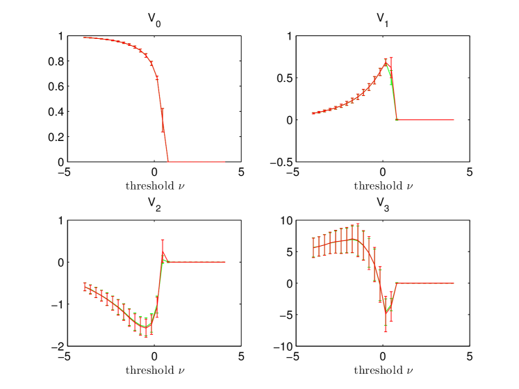
Figure 3: Minkowski functionals of a pure scaling solution of cosmic string wakes, with $G\mu=0.17\times 10^{-6}$. Each of the four boxes shows the results for one of the four functionals, averaged over 100 simulations each using a lattice of $128^{3}$ pixels. Each box contains two curves. corresponding to computing the functionals computed making use of one of the two methods, either Koenderink Invariants (the green curve) or the Crofton Formula (the red curve).

VI.2 Functionals of Noise

We now turn our attention to the Minkowski Functionals of the background noise due to minihalos, shown in Figure 4, where we again calculate the average functionals over 100 simulations and indicate the standard deviation with error bars. The corresponding functionals for a Gaussian random field are shown as the dashed black curves, whereas the functionals for the noise maps are shown in red and green. The key feature of these plots is the symmetry (or antisymmetry in the case of $V_{2}$ and $V_{0}$) about 0, which matches the results for a Gaussian random field. However the noise map functionals all share the common characteristic of being tightly concentrated about 0, which allows the noise map to be differentiated from a pure Gaussian random field. As mentioned above, the deviation of the noise maps from being a pure Gaussian random field comes from the scaling of the amplitude with redshift which is uniform over the two angular coordinates.

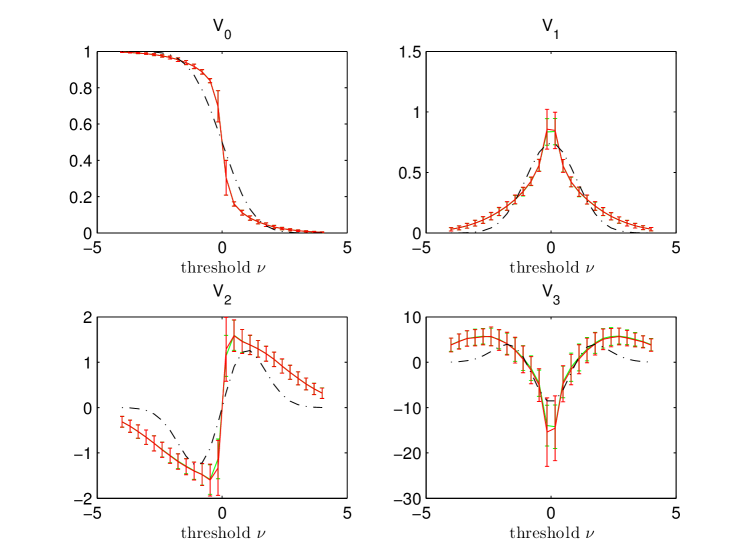
Figure 4: Minkowski functionals of the background noise, averaged over 100 simulations each using a lattice of $128^{3}$ pixels. Each box contains three curves. Two of them are for the noise map with the functionals computed making use of one of two estimates, either Koenderink Invariants (the green curve) or the Crofton Formula (the red curve). The dashed black curves give the Minkowski functionals for a Gaussian map.

VI.3 Functionals of Cosmic Strings Embedded in Noise

Armed with our knowledge of the behaviour of the Minkowski Functionals for both pure cosmic string wake and background noise maps, we can start with the real fun: differentiating maps of wakes and noise from maps of pure noise. To do this, we generate a map of wakes and noise by adding (at every point in space) the temperature fluctuations from wakes and the fluctuations from the mini-halo noise maps. We can then compare the Minkowski functionals as we vary the string tension, allowing us to place constraints on the minimum string tension necessary for the strings to be detected via this method.

For each value of the string tension $G\mu$ we performed 100 simulations. For each simulation we computed the $\chi^{2}$ significance value of the difference between the string and a pure noise map. This was done in the following way: For each threshold bin $i$ (we used $N_{bins}=25$ threshold bins per functional, and hence $4\cdot N_{bins}=100$ bins in total) we computed the probability $p_{i}$ that the Minkowski functional values for the string simulation come from the same distribution as obtained from the pure noise maps. We then combined the results of different bins into a $\chi^{2}$ value using the Fisher combined probability test

$$\chi^{2}=-2\displaystyle\sum_{i=1}^{4N_{bins}}log(p_{i})\,.$$ (41)

We then computed the mean value ${\bar{\chi^{2}}}$ and the standard deviation $\Delta\chi^{2}$ of $\chi^{2}$. The criterion for significance of the difference between string wake and noise maps is that the value of ${\bar{\chi^{2}}}-\Delta\chi^{2}$ is larger than the representative significance value for an analysis with $2(4N_{bins})=200$ degrees of freedom .

A comparison of the functionals of (wakes+noise) against pure noise is shown in Figures 5 to 8, which were done using a lattice size of $128^{3}$, each for a different value of $G\mu$. In each set of graphs, the black curves represent the results for the pure noise maps (the mean values and standard deviations for each threshold value are shown), and the orange curves (the less symmetric - in the case of $V_{1}$ and $V_{3}$ - or less antisymmetric - in the case of $V_{0}$ and $V_{2}$ curves) represent what is obtained for maps containing both strings and noise. What is shown are the Minkowski functionals for a particular cosmic string wake simulation. The mean value of $\chi^{2}$ was found to be greater than $10^{3}$ (the maximal value our numerics could handle) for $G\mu\geq 6.7\times 10^{-8}$, showing that for these values of $G\mu$ string maps can indeed be distinguished from pure noise maps. For $G\mu=4.2\times 10^{-8}$ the $\chi^{2}$ drops down to $223\pm 101$, which indicates a good chance that any one set of wakes+noise will be indistinguishable from the noise at this value of $G\mu$. Hence from this preliminary analysis we conclude that the minimum string tension $G\mu$ must be roughly $5\times 10^{-8}$ for the Minkowski functional method to be able to detect the cosmic string signals which are embedded in the noise.

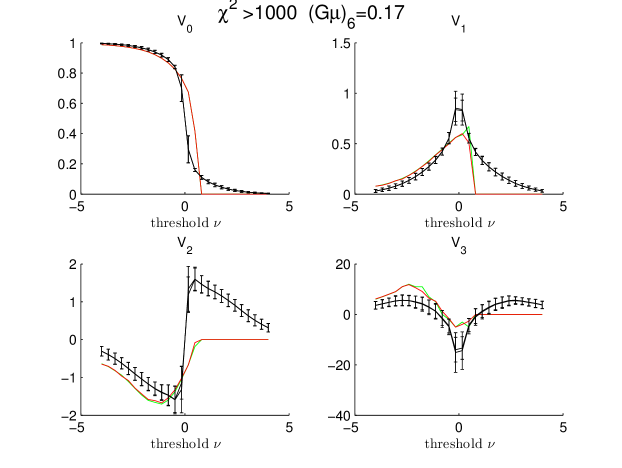
Figure 5: Minkowski functionals of a combined map (wakes+noise) with $G\mu=1.7\times 10^{-7}$ along with the corresponding functionals for a pure noise map, averaged over 100 simulations each using a lattice of $128^{3}$ pixels. The black curves are for the pure noise maps, the orange ones for the strings+noise maps.

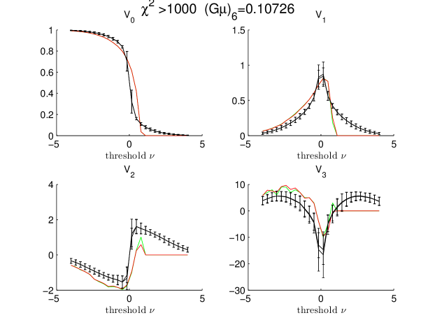
Figure 6: Minkowski functionals of a combined map (wakes+noise) with $G\mu=1.07\times 10^{-7}$ along with the corresponding functionals for a pure noise map, averaged over 100 simulations each using a lattice of $128^{3}$ pixels.

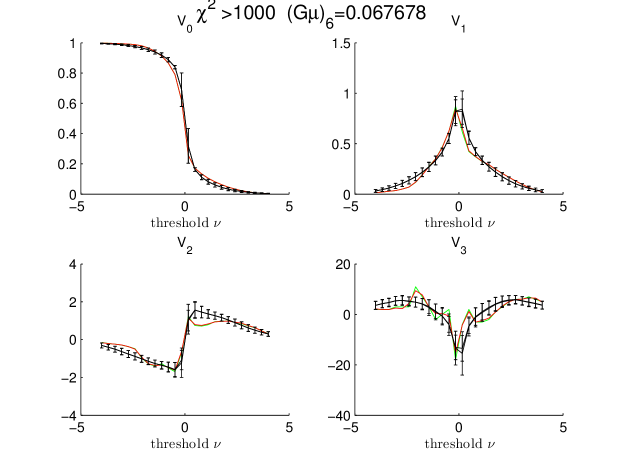
Figure 7: Minkowski functionals of a combined map (wakes+noise) with $G\mu=6.7\times 10^{-8}$ along with the corresponding functionals for a pure noise map, averaged over 100 simulations each using a lattice of $128^{3}$ pixels.

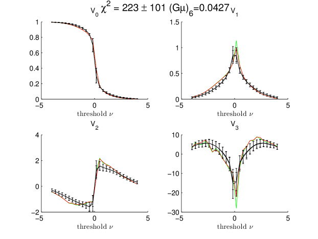
Figure 8: Minkowski functionals of a combined map (wakes+noise) with $G\mu=4.3\times 10^{-8}$ along with the corresponding functionals for a pure noise map, averaged over 100 simulations each using a lattice of $128^{3}$ pixels.

Note the $V_{i}$ values for the cosmic string simulations in Figure 5 vanish to the level of the numerical accuracy above a certain value of the threshold, while those for noise alone do not. The reason this happens is that in the presence of string wakes, a fixed threshold value corresponds to a different brightness temperature than it would in the absence of strings.

Given the limited accuracy of the analysis, we know that the Minkowski functionals at sufficiently close threshold values are not independent. We must thus consider the possibility that we might have oversampled and obtained an artificially large value of $\chi^{2}$. Put another way, since the temperature resolution $\delta T$ of our maps is non-zero, we must account for this in our choice for the threshold bin resolution $\delta\nu$. We can relate $\delta\nu$ and $\delta T$ by

$$\delta\nu=\frac{\delta T}{\sigma_{T}}\,.$$ (42)

The temperature resolution can be estimated to first order by

$$\delta T=\delta x\cdot\nabla T\,,$$ (43)

where $\delta x$ is the spatial resolution and $\nabla T$ is the gradient of the background noise. Since the resolution of the maps is the worst in the redshift direction, we focus on resolution in the $z$-direction. The relevant quantity then is the spatial resolution $\delta l$ corresponding to the redshift resolution $\delta z$, which is given by

$$\delta l(\delta z,z)\sim c(\delta z)t_{0}z^{-3/2}\,.$$ (44)

To then calculate the gradient $\nabla T$, we use the fact that that the matter power spectrum is dominated by modes around $k\sim 1/\lambda_{eq}$, and hence this sets the length scale of the problem. We can then estimate the gradient by

$$T=\frac{\bar{T}}{\lambda_{eq}}\,,$$ (45)

where $\lambda_{eq}$ is

$$\lambda_{eq}\sim ct_{eq}z_{eq}^{-1/2}\,.$$ (46)

Putting this all together we find

$$\delta T\sim\bar{T}\left(\frac{\delta z}{z}\right)\left(\frac{z_{eq}}{z}\right)^{1/2}\sim 0.05\mbox{mK}\,,$$ (47)

where for the second equality we take $z=50$. Using equation 42, this corresponds to $\delta\nu=0.036$. We can then translate that into an upper bound on the number of threshold bins we should use to span 8 standard deviations ($-4\sigma$ to $4\sigma$) and find

$$N_{bins}=\frac{8}{\delta\nu}\sim 200\,.$$ (48)

Hence our choice of 25 threshold bins is well within the limit from oversampling.

Another way to see that the bins can be treated as independent is to consider the correlation matrix for each functional. The correlation matrix is defined by

$$Corr_{ij}=\frac{Cov_{ij}}{\sigma_{i}\sigma_{j}}=\frac{\langle(X_{i}-\mu_{i})(X_{j}-\mu_{j})\rangle}{\sigma_{i}\sigma_{j}}$$ (49)

where the $X_{i}$ are defined by the wake+noise signal for the $i^{\prime}th$ bin. Hence $i$ runs from $1$ to $25$, each $X_{i}$ is a random variable that we have sampled 100 times (once for each trial of the simulation), and $\langle\rangle$ denotes expectation value. From each $X_{i}$ we define a mean $\langle X_{i}\rangle=\mu_{i}$ and a standard deviation $\sigma_{i}$. From this we can calculate the correlation in the wake signal between the bins for each functional, as is plotted in Figure 9. For each functional, the correlation matrix is concentrated in a narrow strip along the diagonal with a width at half max of 2-3 bins. Given this diagonal structure, we are safe from any hidden correlation that would invalidate our use of the Fisher combined probability test.

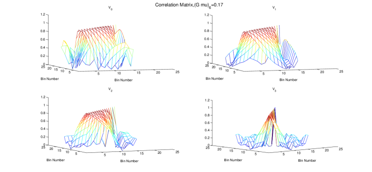
Figure 9: Correlation of wake signal between bins for each functional, using data from 100 realizations.

VII Summary and Outlook

This purpose of this investigation has been to both demonstrate the power of Minkowski Functionals for detecting non-Gaussian behaviour, and to investigate the topology of 21cm distributions in cosmological models with a scaling distribution of cosmic string wakes. We generated 3-D maps of the 21cm brightness temperature in pure cosmic string models, in models with only background noise from mini-halos, and in maps in which both sources of 21cm fluctuations were present, using methods similar to those employed for constructing 2-D CMB temperature by Danos0 . These maps were then be investigated with Minkowski functionals, using the software ‘Minkowski3’ made available by Buchert Buchert . For large values of the string tension, the non-Gaussian signatures of string wakes are clearly visible in the Minkowski functionals. We studied for which range of values of the string tension the difference between the strings + noise versus the pure noise maps as seen in the Minkowski functionals are statictically significant. A large difference was found between the functionals of the string-induced brightness temperature map and the corresponding functionals of background noise, with maps of strings embedded in noise found to be differentiable from maps of pure noise when $G\mu>5\times 10^{-8}$.

The analysis presented in this report serves as a proof of concept that the Minkowski functionals can be used as a statistical tool to search for cosmic string signals. To extend this preliminary analysis would mean performing large scale numerical simulations, as new features may present themselves as we study the 21cm maps with greater resolution.