On the relativistic Lattice Boltzmann method for quark-gluon plasma simulations

Abstract

In this paper, we investigate the recently developed lattice Boltzmann model for relativistic hydrodynamics. To this purpose, we perform simulations of shock waves in quark-gluon plasma in the low and high viscosities regime, using three different computational models, the relativistic lattice Boltzmann (RLB), the Boltzmann Approach Multi-Parton Scattering (BAMPS), and the viscous sharp and smooth transport algorithm (vSHASTA). From the results, we conclude that the RLB model departs from BAMPS in the case of high speeds and high temperature(viscosities), the departure being due to the fact that the RLB is based on a quadratic approximation of the Maxwell-Jüttner distribution, which is only valid for sufficiently low temperature and velocity. Furthermore, we have investigated the influence of the lattice speed on the results, and shown that inclusion of quadratic terms in the equilibrium distribution improves the stability of the method within its domain of applicability. Finally, we assess the viability of the RLB model in the various parameter regimes relevant to ultra-relativistic fluid dynamics.

I Introduction

Recent experiments on heavy-ion (Au-Au) collisions with ultra-relativistic energies at the Relativistic Heavy Ion Collider(RHIC) at Brookhaven National Laboratory, have revealed a new state of matter, the quark-gluon plasma, whereby hadronic matter undergoes a deconfining transition which liberates quarks in the form of a gas of quasi-free particles S. S. Adler et al. (2003). The quark-gluon plasma, which is credited for dominating the primordial state of the Universe in its earliest $1-10$ microseconds, shows very interesting properties, such as near-perfect fluid-like behavior, characterized by ultralow dynamic shear viscosity and associated onset of shock wave propagation Bouras et al. (2009, 2010). The study of such shock waves plays a major role in the characterization of the quark-gluon plasma, since they carry information both on its equilibrium (equation of state) and non-equilibrium (transport coefficients) properties.

In the last years, several numerical tools have been used for the computational investigation of quark-gluon plasmas, such as, for instance: the Boltzmann approach of multiparton scattering (BAMPS) Xu and Greiner (2007), which solves the full Boltzmann equation, $p^{\mu}\partial_{\mu}f(x,p)=C(x,p)$, with $p^{\mu}$ the microscopic 4-momentum vector, $f(x,p)$ the single particle distribution function, and $C(x,p)$ the binary collision term; and the viscous sharp and smooth transport algorithm (vSHASTA)Molnár (2009), which is based on a hydrodynamic description.

Recently, the relativistic lattice Boltzmann (RLB) model Mendoza et al. (2010) was introduced. This new method is a relativistic extension of the classical lattice Boltzmann (LB) equationSucci (2001), whereby a minimal form of the Boltzmann equation is discretized on a lattice and the collision term is applied in a single relaxation time, the so-called Bhatnagar-Gross-Krook approximation, Ref. Bhatnagar et al. (1954)). In the above, ”minimal form”, implies that the particle velocities are constrained to take only a very limited set of discrete values, typically of order $10$ and $20$ in two and three dimensions, respectively (see Fig.1), which represents an enormous simplification as compared to the true Boltzmann equation. The key is that the proper selection of this handful of discrete speeds is sufficient to compute exactly the low-order kinetic moments which characterize the hydrodynamic regime. Crucial to the success of this procedure is that the system be only weakly out of equilibrium, so that the particle distribution function remains close to a local Maxwellian, whose low-order kinetic moments can be computed exactly with just a few suitably chosen discrete velocities (the nodes of Gaussian integration).

The LB method shows many advantages, as for example, the relatively easy implementation of the simulations of fluids in complex geometries, excellent suitability to parallel implementation, and high flexibility towards the inclusion of additional physics, besides sheer hydrodynamics Benzi et al. (1992); Boghosian et al. (1997); Chen and Doolen (1998); Succi et al. (1997); Mazzeo and Coveney (2008). It can thus be expected that the RLB model would carry many of these assets over to the relativistic context. To date, it has been shown to compute shock-wave formation and propagation in quark-gluon plasmas at a fraction of the cost of relativistic hydrodynamic codes Mendoza et al. (2010, 2010).

In order to characterize and improve the RLB model, further studies on its capabilities, limitations and computational performance are in order, which is precisely the focus of this paper. To this purpose, it is worth reminding that the actual RLB model deals with weakly relativistic fluids, characterized by $1<\gamma<2$ and $\zeta\equiv\frac{mc^{2}}{k_{b}T}>1$, where $\gamma=(1-u^{2}/c^{2})^{-1/2}$ is the Lorentz factor associated with a fluid with speed $u$ and $T$ is the fluid temperature. However, since $\gamma=2$ corresponds to $\beta=u/c\sim 0.85$, and $\zeta=1$ associates with ultra-high temperatures, typically above $10^{13}$ Kelvin degrees, the weakly relativistic regime embraces nonetheless a substantial number of interesting applications, including the quark-gluon plasma generated by recent experiments on heavy-ions and hadron jets J. Adams et al. [STAR Collaboration] (2003); A. Adare et al. [PHENIX Collaboration] (2008); F. Wang [STAR Collaboration] (2004); J. Adams et al. [STAR Collaboration] (2005); J. G. Ulery [STAR Collaboration] (2006); N. N. Ajitanand [PHENIX Collabotarion] (2007); A. Adare et al. [PHENIX Collaboration] (2008), as well as astrophysical flows, such as interstellar gas and supernova remnants A. M. Soderberg et al. (2010, 2006).

An extension of the original RLB model, capable of dealing with non-Minkowskian geometries and ultra-relativistic fluids, has been recently developed Romatschke et al. (2011). However, since this method is comparatively more elaborate than the original RLB, in the sequel we shall confine our attention to the latter.

This work is organized as follows: first, in section II we give a short introduction to the RLB model, and show some simulations to validate our implementation. Subsequently, in section  III, we extend the equilibrium distribution function for the particle density, to obtain the correct density profile in the moderately relativistic regime $\gamma\sim 2$. Finally, in section  IV, we analyze the effect of the lattice speed on the results, provide comparisons in the moderately relativistic and high viscosity regimes with the previous mentioned methods, BAMPS and vSHASTA, and assess the viability of this scheme for ultra-relativistic fluid dynamics.

II Relativistic lattice Boltzmann model

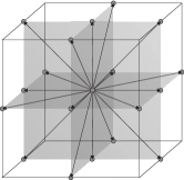
Figure 1: The D3Q19 (19 speeds in 3 dimensions) cell configuration. Every arrow corresponds to the scaled velocity vector $\delta t\vec{c}_{i}$, and the points correspond to the discretized space coordinates $\vec{x}$.

In this section, we describe the relativistic lattice Boltzmann, which is the basis of this work, develop some improvements and test the new implementation against known results for the Riemann problem. The Riemann problem has piecewise constant initial conditions and a single discontinuity, and is commonly used to test numerical methods that model systems with conservation laws.

II.1 Conservation laws for relativistic fluid dynamics

The conservation laws for relativistic fluid dynamics, which our RLB model is based upon, are: the conservation of particle density (in a relativistic regime mass is not invariant), and the energy momentum conservation, which has to be treated separately in contrast to the classical LB.

The conservation of the particle number density $n$ is given by:

$$\partial_{t}\left(n\gamma\right)+\partial_{a}\left(n\gamma u_{a}\right)=0\quad,$$

where $\vec{u}$ denotes the macroscopic fluid velocity. Here, Latin indices denote the three dimensional space coordinates. Note that in the following the speed of light $c$ and the Boltzmann constant $k_{b}$ are taken to be unity for notational simplicity. As a result, $\beta=u$ and $\zeta=m/T$. Also we use the Einstein summation, i.e. repeated indices are summed upon. The hydrodynamic equations for the energy momentum conservation read as follows:

$$\partial_{t}\left(\left(\epsilon+P\right)\gamma^{2}-P\right) +\partial_{a}\left(\left(\epsilon+P\right)\gamma^{2}u_{a}\right)$$ (1)

$$+\partial_{t}\pi^{00}+\partial_{a}\pi^{ab}=0\quad,$$

$$\partial_{t}\left(\left(\epsilon+P\right)\gamma^{2}u_{ab}\right) +\partial_{b}P+\partial_{a}\left(\left(\epsilon+P\right)\gamma^{2}u_{a}u_{b}\right)$$

$$+\partial_{t}\pi^{0b}+\partial_{b}\pi^{ab}=0\quad,$$

where $\epsilon$ is the energy density, $P$ is the hydrostatic pressure, and $\pi^{ab}$ are the components of the dissipation stress-energy tensor. Here the $0$ index denotes the time component.

II.2 Implementation of the RLB scheme

We implement the relativistic lattice Boltzmann model along the lines proposed in Refs.Mendoza et al. (2010, 2010). This model is based on two density distribution functions, $f_{i}$ and $g_{i}$, which are associated to a D3Q19 lattice Succi (2001) (see Fig. 1), with $19$ discrete velocities $\vec{c}_{i}$ in $d=3$ dimensions.

These velocities take just the values $0,\pm c_{l}$, where $c_{l}=\frac{\delta x}{\delta t}$ is the lattice speed. Each discrete velocity $c_{i}$ is associated with a corresponding discrete distribution function, $f_{i}(\vec{x},t)\equiv f(\vec{x},t;\vec{p}_{i})$ for the fluid density, and $g_{i}(\vec{x},t)\equiv g(\vec{x},t;\vec{p}_{i})$, with $\vec{p}_{i}=m\gamma_{i}\vec{c}_{i}$, for the fluid energy-momentum.

The distributions evolve according to the following discrete BGK Boltzmann equations Bhatnagar et al. (1954):

$$f_{i}(\vec{x}+\vec{c}_{i}\delta t,t+\delta t)-f_{i}(\vec{x},t)=-\frac{\delta t}{\tau}(f_{i}-f_{i}^{\rm eq})\quad,$$ (2a)

$$g_{i}(\vec{x}+\vec{c}_{i}\delta t,t+\delta t)-g_{i}(\vec{x},t)=-\frac{\delta t}{\tau}(g_{i}-g_{i}^{\rm eq})\quad,$$ (2b)

where $\tau$ represents the local relaxation time, $f_{i}^{\rm eq}$ and $g_{i}^{\rm eq}$ are the equilibrium distribution functions.

The above equations describe a two-step lattice dynamics. The left-hand side encodes the free-streaming of the distributions along the characteristics defined by the discrete velocities $\vec{c}_{i}$. Note that since velocities are constant in space and time, this term is an exact lattice transcription of the free-streaming term in the continuum Boltzmann equation. This leads to major benefits for the computational performance of the model because, at variance with hydrodynamic formulations, the information always travels along straight lines rather than along space-time changing material fluid lines.

The right-hand side describes particle collisions in the form of a relaxation towards local equilibria, on a time scale $\tau$. This is the lattice analogue of the relativistic Marle model Marle (1965).

In order for the relativistic LB equations (Eq. (2)) to correctly reproduce relativistic hydrodynamics in the continuum limit, the lattice equilibria have to be designed in compliance with the basic number-energy-momentum conservation laws. As shown in Ref. Mendoza et al. (2010), this can be accomplished through an algebraic moment-matching procedure, leading to the following expressions:

$$f_{i}^{\rm eq} =w_{i}n\gamma\left(1+3\frac{(\vec{c}_{i}\cdot\vec{u})}{c_{l}^{2}}\right)\quad,$$ (3)

$$g_{0}^{eq} =3w_{0}P\gamma^{2}\left(4-\frac{2+c_{l}^{2}}{\gamma^{2}c_{l}^{2}}-2\frac{|\vec{u}|^{2}}{c_{l}^{2}}\right)\quad,$$

$$g_{i>0}^{eq} =3w_{i}P\gamma^{2}\left(\frac{1}{\gamma^{2}c_{l}^{2}}+4\frac{(\vec{c}_{i}\cdot\vec{u})}{c_{l}^{2}}+6\frac{(\vec{c}_{i}\cdot\vec{u})^{2}}{c_{l}^{4}}-2\frac{|\vec{u}|^{2}}{c_{l}^{2}}\right)\quad,$$

The above probability distribution functions recover the macroscopic values, with the ultra-relativistic state equation $\epsilon=3P$, provided the following identifications are made:

$$n =\frac{1}{\gamma}\sum_{i}f_{i}\quad,$$ (4)

$$P =-\frac{1}{3}\sum_{i}g_{i}+\frac{1}{3}\sqrt{-3\left(\sum_{i}g_{i}\vec{c}_{i}\right)^{2}+4\left(\sum_{i}g_{i}\right)^{2}}\quad,$$ (5)

$$\vec{u} =\frac{1}{3\sum_{i}g_{i}+3P}\sum_{i}g_{i}\vec{c}_{i}\quad.$$ (6)

In the above, the discrete weights take the value $w_{0}=1/3$, for $|\vec{c}_{0}|=0$, $w_{i}=1/18$ for $|\vec{c}_{i}|=c_{l}$, and $w_{i}=1/36$ for $|\vec{c}_{i}|=\sqrt{2}c_{l}$. Based on these expressions, it is readily checked that $\sum_{i}w_{i}=1$ and $c_{s}^{2}=\sum_{i}w_{i}c_{ia}^{2}=\frac{c_{l}^{2}}{3}$, where $a=x,y,z$. The latter defines the sound speed, $c_{s}$, and shows that, by stipulating $c_{l}=c$, i.e. the lattice speed equal to the light speed, the RLB supports the relativistic ideal equation of state $c_{s}^{2}=\frac{c^{2}}{3}$.

It is worth emphasizing that, unlike local equilibria in continuum momentum space, lattice equilibria are not unconditionally positive for any value of the fluid velocity. This is because continuum equilibria, both non-relativistic (Maxwell-Boltzmann) and relativistic (Maxwell-Juettner), are irrational functions of both the microscopic and hydrodynamic velocity (four-momentum). This is no accident, but rather the result of the local equilibria following from an entropy minimization principle, with the entropy additivity imposing a non-rational (exponential) functional dependence on the collision invariants Liboff (1969). Hence, an exact transcription of such equilibria would require an infinite series in powers of $u/c_{s}$. However, since the generic $n$-th term of such an expansion involves $n$-th order tensors of the form $\sum_{i}\vec{c}_{i}\vec{c}_{i}\dots\vec{c}_{i}$, it is clear that much larger symmetry groups, i.e. much more discrete velocities, would be needed at each step of the expansion. This would rapidly lead to an unmanageable complexity. It is quite fortunate that hydrodynamics can be reproduced by ensuring the correct symmetry of just fourth-order tensors, so that, relatively simple lattices like the D3Q19, can accomplish the task. Failing such fortunate circumstance, no LB would ever exist.

To model shock waves in viscous quark-gluon matter, this scheme has to recover a special viscosity-entropy density ratio $\frac{\eta}{s}$, where the entropy density $s$ is approximated by $s=4n-n\ln\lambda$, with $\lambda=\frac{n}{n^{eq}}$ and $n^{eq}=\frac{d_{G}T^{3}}{\pi^{2}}$ ($d_{G}=16$ is the degeneration for gluons and $T$ is the temperature) Bouras et al. (2009).

The dynamic viscosity can be computed from the relaxation time according to the following expression:

$$\eta=\frac{4}{3}c_{l}^{2}\gamma P(\tau-\frac{\delta t}{2})$$ (8)

The term $c_{l}^{2}(\tau-\frac{\delta t}{2})$ is standard from conventional Lattice Boltzmann theory. However, in contrast to the classical Lattice Boltzmann method, this term is pre-factored by $\gamma P/c^{2}$ ($c=1$ in our units) rather than by fluid density $\rho$.

For the purpose of this work, $\tau$ is computed with the initial $P$ and $\gamma$, so as to obtain the desired $\frac{\eta}{s}$ ratio. Note that the initial $P$ and $\gamma$, in general for the Riemann problem, are functions of the coordinates, so they can lead to a spatially dependent relaxation time $\tau$. To avoid this, we have used their spatial averages.

II.3 Numerical validation

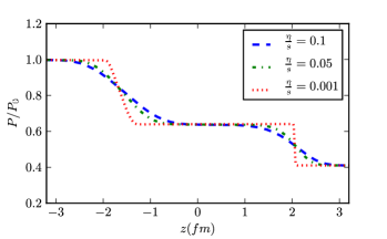
(a) Pressure

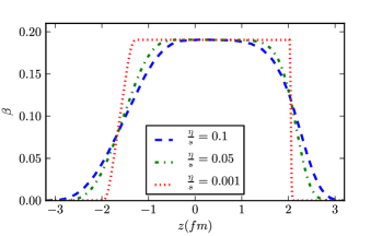
(b) Velocity

Figure 2: Pressure and velocity profiles for different $\frac{\eta}{s}$ ratios, at $t=3.2\frac{fm}{c}$. The profiles show excellent agreement with the results in Ref.Mendoza et al. (2010).

In order to test our numerical scheme, we carry out some simulations of shock waves in quark-gluon plasmaBouras et al. (2009) in one dimension, and compare the results with the existing literature, Ref. Mendoza et al. (2010). For this simulation, a lattice with $1\times 1\times 800$ cells, open boundaries along the mainstream $z$-direction and periodic boundaries along the cross-flow $x$-and $y$-directions are used. As a result, we set $\delta x=0.008fm$ and $\delta t=0.008\frac{fm}{c}$. The initial conditions for the pressure are $P(z<0)=P_{0}=5.43\frac{GeV}{fm^{3}}$ and $P(z\geq 0)=P_{1}=2.22\frac{GeV}{fm^{3}}$. This corresponds, in numerical units, to $2.495\times 10^{-7}$ and $1.023\times 10^{-7}$, respectively. The initial temperature is constant over the whole domain having the value $350MeV$ (in numerical units $0.0314$), corresponding to $\zeta\sim 3$.

The initial particle density is computed through the relation $n=\frac{P}{T}$. The pressure and velocity profiles at $3.2\frac{fm}{c}$ for different $\frac{\eta}{s}$ ratios between $0.001$ and $0.1$, are shown in Fig. 2, from which excellent agreement with the results in Ref.Mendoza et al. (2010) is readily appreciated. Each simulation took around one second on a Intel core i5 of 2.3GHz.

III Improving the equilibrium distribution

Figure 3: Comparison of the particle density using both equilibrium functions, Eqs. (3) and (9), at $t=3.2\frac{fm}{c}$, with the initial conditions given in section IV.1, $\frac{\eta}{s}=0.005$, and $c_{l}=1$. As one can appreciate, the density profiles are basically the same.

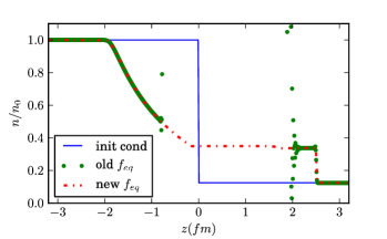
Figure 4: Comparison of the particle density using both equilibrium functions, at $t=3.2\frac{fm}{c}$, with the initial conditions given in section IV.2, $\frac{\eta}{s}=0.001$, and $c_{l}=1$. The result obtained with the old (linear) equilibrium function breaks down in the region $z\in[-1,2]$, whereas for the case of the new (quadratic) equilibrium function, the model reproduces the correct profile in the whole domain.

Inspection of the particle density equilibrium distribution function, $f_{i}^{\rm eq}$$=$$w_{i}n\gamma\left(1+3\frac{(\vec{c}_{i}\cdot\vec{u})}{c^{2}_{l}}\right)$, shows that this becomes negative for counter-streaming populations when $(\vec{c}_{i}\cdot\vec{u})<-\frac{c_{l}^{2}}{3}$. This is non-physical and leads to either unreliable results (see Fig. 4) or numerical instability.

In previous works Mendoza et al. (2010, 2010), this problem was circumvented by increasing the lattice speed $c_{l}$ and reducing the time step accordingly, so that the light-cone condition $c_{l}\delta t=\delta x$, remained fulfilled. In the low-viscosity regime this was found to stabilize the numerics without affecting the physics to any appreciable extent. However, as shown in the sequel, in at higher viscosities, this is no longer the case.

A detailed analysis of the effect of the lattice speed on the physical results is presented in section IV. However, prior to this, we first introduce a new particle density equilibrium function, which allows larger fluid velocities at a given value $c_{l}=1$, without violating the positivity condition, $f_{i}^{\rm eq}>0$.

This new equilibrium distribution reads as follows:

$$f_{i}^{\rm eq}=\omega_{i}n\gamma\left(1+3\frac{(\vec{c}_{i}\cdot\vec{u})}{c_{l}^{2}}+\frac{9}{2}\frac{(\vec{c}_{i}\cdot\vec{u})^{2}}{c_{l}^{4}}-\frac{3}{2}\frac{|\vec{u}|^{2}}{c_{l}^{2}}\right)\quad.$$ (9)

This expression includes a new quadratic term in the macroscopic fluid velocity. This new term is standard in classical lattice Boltzmann theory, and results form second order expansion in the fluid velocity of a locally shifted Maxwellian distribution $\sim e^{-\frac{m(v-u)^{2}}{2kT}}$.

To check that the new equilibrium function is valid and reproduces the same results as the old one, we carry out several simulations in the weakly relativistic regime, which each of them required around one second on an Intel core i5 of 2.3GHz. For illustration purposes, we show just one example, where we only consider the particle distribution function, because the improved equilibrium function has no direct influence neither on the pressure nor on the velocities, see Eq. (4).

From Fig. 3, which shows that density profile at $\eta/s=5\;10^{-3}$, we observe that both equilibrium distribution functions give basically the same result. However, from Fig. 4, which refers to $\eta/s=10^{-3}$, we can see that the computation of the particle density using the old equilibrium distribution function, in the moderately relativistic regime, is breaking down in the region $z\in[-1,2]fm$, and leads to very large fluctuations, with both positive and negative values. For visualization purposes, just the physically meaningful region is plotted. Note that outside of the region $z\in[-1,2]fm$ both equilibrium functions reproduce the same result. However, in the course of the evolution, those fluctuations are found to propagate over the entire simulation domain.

IV Influence of the lattice speed

Having illustrated the stabilization effects of the new equilibrium distribution, all following numerical experiments are performed with this distribution. Next, we study the influence of the lattice speed, $c_{l}$. For this purpose, we simulate various shock waves in quark-gluon plasma with different viscosity-entropy density ratios and different lattice speeds in the weak ($1<\gamma\ll 2$) and mildly ($\gamma\sim 2$) relativistic regimes. As noted before, by increasing the lattice speed, we need to decrease the time step, in such a way that $\vec{x}+\vec{c}_{i}dt$ corresponds to a grid point in the lattice. Basically, in numerical units, $c_{l}=10$ implies $dt=0.1$, so that the product is always $1$ or $\sqrt{2}$, depending of the velocity vector $\vec{c}_{i}$. Clearly, smaller time-steps imply a correspondingly larger number of time steps, hence more simulation time.

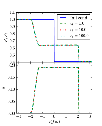
Figure 5: Weakly relativistic case, $\frac{\eta}{s}=0.001$. Pressure and velocity profiles for different lattice speeds at $t=3.2\frac{fm}{c}$. In this case, the choice of the lattice speed does not affect the result of the simulation.

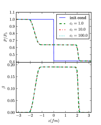
Figure 6: Weakly relativistic case, $\frac{\eta}{s}=0.005$. Pressure and velocity profiles for different lattice speeds and , at $t=3.2\frac{fm}{c}$. Here, some differences are visible.

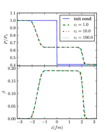
Figure 7: Weakly relativistic , $\frac{\eta}{s}=0.01$. Pressure and velocity profiles for different lattice speeds at $t=3.2\frac{fm}{c}$. Here we observe a small effect of the lattice speed.

IV.1 Weakly relativistic regime, $\gamma\ll 2$

For the weakly relativistic simulations, we use a lattice with $1\times 1\times 800$ cells, open boundaries in $z$-direction and periodic boundaries in $x$-and $y$-direction. We set $\delta x=0.008fm$ and $\delta t=\frac{0.008}{c_{l}}\frac{fm}{c}$. The initial conditions for the pressure are $P(z<0)=P_{0}=5.43\frac{GeV}{fm^{3}}$ and $P(z\geq 0)=P_{1}=2.22\frac{GeV}{fm^{3}}$. This corresponds in numerical units to $2.495\times 10^{-7}$ and $1.023\times 10^{-7}$, respectively. The initial temperature is constant over the whole domain, namely $400MeV$(in numerical units $0.036$), corresponding to $\zeta\sim 2.5$. The initial particle density is calculated with the equation of state, $n=\frac{p}{T}$.

A snapshot of the pressure and velocity profiles at $t=3.2\frac{fm}{c}$, for different lattice speeds($c_{l}=1$, $c_{l}=10$, and $c_{l}=100$) and different viscosity-entropy ratios (between $0.001$ and $0.01$), is shown in Figs. 5, 6 and 7. From these figures, we can observe that , as expected based on previous experience, there is no significant effect of the lattice speed on the results. However, there is a significant difference in the computational performance, the simulations took around $1$, $9$, and $90$ seconds for $c_{l}=1.0$, $c_{l}=10.0$ and $c_{l}=100.0$, respectively.

IV.2 Moderately relativistic regime, $\gamma\sim 2$

For the moderately relativistic regime, we perform the simulations on a lattice with $1\times 1\times 1600$ cells, in order to cover a larger computational domain. The same boundaries are used as before. We set $\delta x=0.008fm$ and $\delta t=\frac{0.008}{c_{l}}\frac{fm}{c}$. The initial conditions for the pressure are $P_{0}=5.43\frac{GeV}{fm^{3}}$ and $P_{1}=0.339\frac{GeV}{fm^{3}}$. In numerical units, they correspond to $2.495\times 10^{-7}$ and $1.557\times 10^{-8}$, respectively. The initial temperature is now different for $z\geq 0$ namely $T_{1}=200MeV$ (in numerical units $0.018$), corresponding to $\zeta\sim 5$.

For $z<0$ the initial temperature is the same as in the previous simulation, $T_{0}=400MeV$ (in numerical units $0.036$), and the initial particle density is computed in the same way as before. The velocity and pressure profiles at $t=3.2\frac{fm}{c}$, for different lattice speeds($c_{l}=1$, $c_{l}=10$, and $c_{l}=100$) and different viscosity-entropy density ratios ($0.001$ and $0.05$), are shown in Figs.  8 and 9. Again, no significant influence of the lattice speed is observed.

For $\frac{\eta}{s}=0.01$, we perform the simulation using a lattice with $1\times 1\times 800$ cells, so that $\delta x=0.016fm$ and $\delta t=\frac{0.016}{cl}\frac{fm}{c}$. In this case, the numerical units of the pressure are $P_{0}=1.996\times 10^{-6}$ and $P_{1}=1.2456\times 10^{-7}$, respectively. The numerical values of the temperatures and particle density are set up in the same way as before. The results of this simulation are shown in Fig.  10. Here, we see that the lattice speed drastically affects the results. The implemented simulation in this section spanned around $1$, $4$, and $44$ seconds for the cases $c_{l}=1.0$, $c_{l}=10.0$, and $c_{l}=100.0$, respectively.

Summarizing, we conclude that the physical results in the moderately relativistic regime are affected by the increasing value of the lattice speed beyond $c_{l}=1.0$. Also, we see that this effect is more pronounced with increasing $\frac{\eta}{s}$. Furthermore, we observe that the results of the simulation with high lattice speeds, for a given ratio $\frac{\eta}{s}$, are similar to the ones obtained with $c_{l}=1$ for a higher viscosity-entropy density ratio. To understand this effect, a deeper theoretical investigation of the basic RLB scheme is required. According to the Chapman-Enskog expansion, the relation for $\eta$ results from a Taylor expansion of the discrete lattice Boltzmann equation to second order in space and time, combined with a first order perturbation in the Knudsen number $Kn\sim c_{s}\tau/\delta x=\frac{1}{3}\tau/\delta t$, and quadratic truncation of the local equilibria in the Mach number $Ma=u/c_{s}=\sqrt{3}\beta$. Since, as we have observed before, raising $c_{l}$ implies lowering $\delta t$, it is clear that simulations with $c_{l}>1$ at a given $\tau$, imply larger values of the Knudsen number, thus pushing RLB potentially outside of the domain of validity of the Chapman-Enskog asymptotics. Similar problems are well known to occur in the simulation of complex non-relativistic fluids with sharp interfaces Sbragaglia et al. (2007).

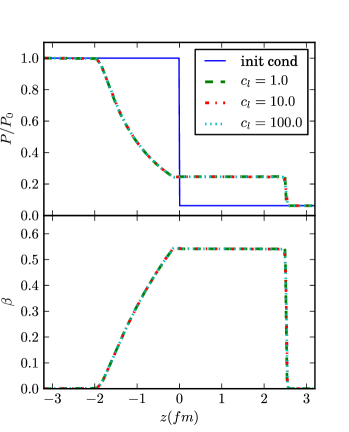
Figure 8: Moderately relativistic case, $\frac{\eta}{s}=0.001$. Pressure and velocity profiles for different lattice speeds at $t=3.2\frac{fm}{c}$. Very small differences appear only at the highest $\beta$.

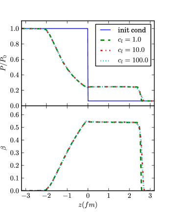
Figure 9: Moderately relativistic case, $\frac{\eta}{s}=0.005$. Pressure and velocity profiles for different lattice speeds at $t=3.2\frac{fm}{c}$. Here we see some differences for different lattice speeds.

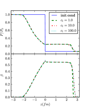
Figure 10: Moderately relativistic case, $\frac{\eta}{s}=0.01$. Pressure and velocity profiles for different lattice speeds at $t=3.2\frac{fm}{c}$. Here we observe, that especially for the highest $\beta$, the results differ substantially.

V Comparison with BAMPS and vSHASTA for high values of $\frac{\eta}{s}$

In this section, we perform simulations to compare the RLB model with BAMPS and vSHASTA Bouras et al. (2010) for the case of high viscosities and high speeds. The initial conditions are the same as in section IV.2. We use $c_{l}=1.0$ and a lattice with $1\times 1\times 1600$ cells, so that the numerical units stay the same. Each simulation took around one second on an Intel core i5 of 2.3GHz. The results of the simulation at $t=3.2\frac{fm}{c}$ for two different viscosities are shown in Figs. 11 and 12.

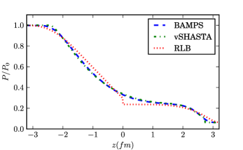
(a) Pressure

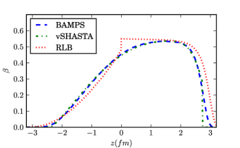
(b) Velocity

Figure 11: Pressure and velocity profiles for the different models with $\frac{\eta}{s}=0.1$. BAMPS and vSHASTA show only tiny departures from each other, but differ significantly from RLB.

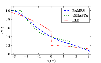
(a) Pressure

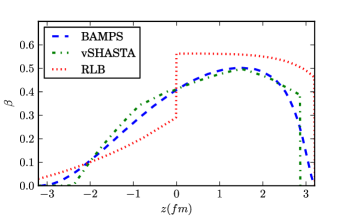
(b) Velocity

Figure 12: Pressure and velocity profiles for the different models with $\frac{\eta}{s}=0.5$. vSHASTA has stability problems and discontinuities, while the RLB diverges from the BAMPS solution even more.

Due to the fact that BAMPS is the solution of the Boltzmann equation with the complete collision term, while the RLB model is a near-equilibrium approximation, and vSHASTA is a second order scheme for modeling relativistic fluid dynamics, it is very interesting to compare the three techniques with each other.

For $\frac{\eta}{s}=0.1$ the results from BAMPS and vSHASTA are very close, and the RLB presents some small deviations. On the other hand, for $\frac{\eta}{s}=0.5$, BAMPS still reproduces stable results, whereas vSHASTA suffers some stability problems and discontinuities, and the deviations of the RLB become more pronounced. To understand these deviations in high viscosity regime, we start first by revisiting the meaning of the viscosity-entropy density ratio within the RLB model. The viscosity-entropy density ratio can be written as

$$\frac{\eta}{s}=\frac{\frac{4}{3}\gamma P\left(\tau-\frac{\delta t}{2}\right)c_{l}^{2}}{n\left(4-\ln\left(\frac{n\pi^{2}}{d_{G}T^{3}}\right)\right)}\quad,$$ (10)

and using the relation $T=\frac{P}{n}$,

$$\frac{\eta}{s}=\frac{\gamma c_{l}^{2}\left(\tau-\frac{\delta t}{2}\right)}{3+\frac{9}{4}\ln\left(\sqrt[3]{\frac{d_{G}}{n\pi^{2}}}T\right)}T\quad.$$ (11)

This expression shows that, for high temperatures, there is a nearly linear dependence of $\frac{\eta}{s}$ on the temperature, which means that when we simulate a high $\frac{\eta}{s}$ ratio, this corresponds, in terms of the Boltzmann equation, to a high equilibrium temperature.

Note that the results of the RLB simulations present a discontinuity at $z=0$ fm in Figs. 11 and 12. This discontinuity appears as a consequence of the initial condition for the pressure (solid line in Fig. 10), which is set according to the Riemann problem. Therefore, we can conclude that the RLB, in the case of high viscosity-entropy density ratios, is not able to solve correctly the Riemann problem and maintains the initial discontinuity during the whole simulation.

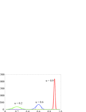
Figure 13: Maxwell-Jüttner distribution for different velocities at very low temperatures, $mc^{2}/kT=200$, the dashed lines denote the parabolic approximation to the respective MJ distribution, denoted by solid lines. Only the positive velocities are shown since the distribution is symmetric.

The RLB model approximates the probability equilibrium distribution functions by a quadratic expression, i..e a parabolic approximation. At sufficiently low temperature, this approximation is accurate, but as temperature is increased, hence higher values $\frac{\eta}{s}$, accuracy is rapidly lost. To appreciate this effect, it is instructive to graphically inspect the Maxwell-Jüttner distribution (MJ)Cercignani and Kremer (2002) $f_{MJ}(\vec{x},\vec{p},t)=\frac{1}{Z}\exp\left(-\frac{U^{\alpha}p_{\alpha}}{T}\right)$, which depends on the macroscopic four-velocity $U^{\alpha}=\gamma(\vec{u})\left(1,\vec{u}\right)$, and the microscopic four-momentum $p_{\alpha}=\gamma(\vec{v})m\left(1,-\vec{v}\right)$, where $m$ is the rest mass and $\vec{v}$ the microscopic velocity and $Z$ a normalization factor that depends on the temperature and macroscopic velocity.

From Figs. 13, 14 and 15, we observe that the MJ distribution becomes broad and very asymmetric for high velocities and high temperatures, and therefore a parabolic approximation is no longer valid. In fact, at $\zeta<1$, the parabolic approximation should be replaced by a bimodal parabolic one, which is certainly feasible, but beyond the current RLB formulation. This explains why RLB has problems to reproduce results in this regime. However, for the case of low temperature and relatively high velocities, the RLB model can still model the proper fluid dynamics since its equilibrium distribution functions (parabolic approximation) remain very close to the MJ distribution. For high temperatures, it is only possible to study weakly relativistic systems (see Fig. 15).

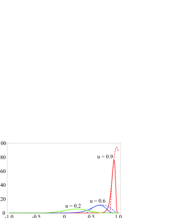
Figure 14: Maxwell-Jüttner distribution for different velocities at low temperatures, $mc^{2}/kT=20$, the dashed lines represent the parabolic approximation to the respective MJ distribution, denoted by solid lines.

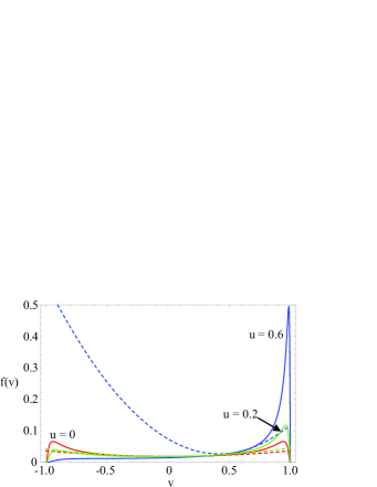
Figure 15: Maxwell-Jüttner distribution for different velocities at high temperatures, $mc^{2}/kT=1$, the dashed lines denote the parabolic approximation to the corresponding MJ distribution (solid lines).

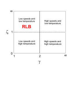
Figure 16: Qualitative sketch of the four different regimes characterized by the parameters $\zeta=mc^{2}/kT$, and $\gamma=1/\sqrt{1-\vec{u}^{2}}$. Our RLB model lies in the region of low temperatures, $\zeta>1$ and $\gamma<2$.

As a general conclusion, we expect that the RLB approach can model moderately-relativistic fluid dynamics ($|\vec{u}|\approx 0.9$) only in the low temperature regime, $\zeta>1$. For illustration purposes, we show a qualitative sketch of the regimes characterized by the parameters $\zeta$ and $\gamma$ in Fig. 16.

VI Conclusion

Summarizing, in this paper we have determined the capabilities and limitations of the RLB model for the simulation of relativistic flows in the various regimes associated to the flow speed and temperature. For this purpose, we have performed extensive simulations of shock waves in quark-gluon plasma at weakly and moderately relativistic regimes and low and high viscosities. We have introduced a higher order equilibrium distribution function, which is shown to enhance the stability of the original RLB model, and permits to compute correctly the particle density profile in the moderately relativistic regime, with no need of enhancing the lattice speed, hence no need of reducing the time-step, as in the original RLB model. The result is that RLB can compute well-resolved weakly and moderately one-dimensional relativistic shock wave propagation in less than a minute, CPU time on an Intel core i5 of 2.3Ghz. To the best of our knowledge, this is significantly faster than any hydrodynamic code, let alone the full BAMPS solution.

Furthermore, we have performed a numerical investigation of the effect of the lattice speed on the physical results, and concluded that the results can differ, due to higher order terms in the dissipation tensor which are not included in the Chapman-Enskog analysis. As a consequence, we observed that the results of the simulation with high lattice speeds, for a given ratio $\frac{\eta}{s}$, are similar to the ones obtained with $c_{l}=1$ for a higher viscosity-entropy density ratio.

In this study, we also showed that the choice of high viscosity-entropy density ratios at high speeds, affects the accuracy of the results. In addition, by direct comparison of the current RLB model with BAMPS and vSHASTA in a moderately relativistic and highly viscous regime, we have shown that the parabolic approximation of the Maxwell-Juettner distribution poses significant restrictions to the viability of RLB for strongly relativistic, high temperature, fluids.

Finally, based on the study of the approximation of the MJ distribution with parabolic equilibria, we are led to predict, that the current RLB model would properly work at relatively low temperatures, $\zeta>1$, and high velocities ($\beta\sim 0.9$). Fortunately, such regimes are by no means devoid of interesting physical applications. Extension to more general relativistic flows requires further developments, such as the introduction of higher order lattices, with higher order equilibria, possibly equipped with relativistic H-theorems (entropic LB methods). This offers a very interesting object of future research in the field.

References

- S. S. Adler et al. (2003) S. S. Adler et al. (PHENIX Collaboration), Phys. Rev. Lett., 91, 182301 (2003).
- Bouras et al. (2009) I. Bouras, E. Molnár, H. Niemi, Z. Xu, A. El, O. Fochler, C. Greiner, and D. H. Rischke, Phys. Rev. Lett., 103, 032301 (2009).
- Bouras et al. (2010) I. Bouras, E. Molnár, H. Niemi, Z. Xu, A. El, O. Fochler, C. Greiner, and D. H. Rischke, Phys. Rev. C, 82, 024910 (2010).
- Xu and Greiner (2007) Z. Xu and C. Greiner, Phys. Rev. C, 76, 024911 (2007).
- Molnár (2009) E. Molnár, The European Physical Journal C - Particles and Fields, 60, 413 (2009).
- Mendoza et al. (2010) M. Mendoza, B. M. Boghosian, H. J. Herrmann, and S. Succi, Phys. Rev. Lett., 105, 014502 (2010a).
- Succi (2001) S. Succi, The Lattice Boltzmann Equation for Fluid Dynamics and Beyond (Oxford University Press, 2001).
- Bhatnagar et al. (1954) P. L. Bhatnagar, E. P. Gross, and M. Krook, Phys. Rev., 94, 511 (1954).
- Benzi et al. (1992) R. Benzi, S. Succi, and M. Vergassola, Physics Reports, 222, 145 (1992), ISSN 0370-1573.
- Boghosian et al. (1997) B. Boghosian, F. Alexander, and P. Coveney, Int. J. Mod. Phys. C, 8 (1997).
- Chen and Doolen (1998) S. Chen and G. D. Doolen, Annual Review of Fluid Mechanics, 30, 329 (1998).
- Succi et al. (1997) S. Succi, G. Amati, and R. Piva, Int. J. Mod. Phys. C, 8, 869 (1997).
- Mazzeo and Coveney (2008) M. Mazzeo and P. Coveney, Computer Physics Communications, 178, 894 (2008), ISSN 0010-4655.
- Mendoza et al. (2010) M. Mendoza, B. M. Boghosian, H. J. Herrmann, and S. Succi, Phys. Rev. D, 82, 105008 (2010b).
- J. Adams et al. [STAR Collaboration] (2003) J. Adams et al. [STAR Collaboration], Phys. Rev. Lett., 91, 172302 (2003).
- A. Adare et al. [PHENIX Collaboration] (2008) A. Adare et al. [PHENIX Collaboration], Phys. Rev. Lett., 101, 232301 (2008a).
- F. Wang [STAR Collaboration] (2004) F. Wang [STAR Collaboration], J. Phys. G, 30, S1299 (2004).
- J. Adams et al. [STAR Collaboration] (2005) J. Adams et al. [STAR Collaboration], Phys. Rev. Lett., 95, 152301 (2005).
- J. G. Ulery [STAR Collaboration] (2006) J. G. Ulery [STAR Collaboration], Nucl. Phys. A, 774, 581 (2006).
- N. N. Ajitanand [PHENIX Collabotarion] (2007) N. N. Ajitanand [PHENIX Collabotarion], Nucl. Phys. A, 783, 519 (2007).
- A. Adare et al. [PHENIX Collaboration] (2008) A. Adare et al. [PHENIX Collaboration], Phys. Rev. C, 78, 014901 (2008b).
- A. M. Soderberg et al. (2010) A. M. Soderberg et al., Nature Letters, 463, 513 (2010).
- A. M. Soderberg et al. (2006) A. M. Soderberg et al., Nature Letters, 442, 1014 (2006).
- Romatschke et al. (2011) P. Romatschke, M. Mendoza, and S. Succi, Accepted for publication in Phys. Rev. C (2011).
- Marle (1965) C. Marle, C. R. Acad. Sc. Paris, 260, 6539 (1965).
- Liboff (1969) R. Liboff, Introduction to the Theory of Kinetic Equations (New York: Wiley, 1969).
- Sbragaglia et al. (2007) M. Sbragaglia, R. Benzi, L. Biferale, S. Succi, K. Sugiyama, and F. Toschi, Phys. Rev. E, 75, 026702 (2007).
- Cercignani and Kremer (2002) C. Cercignani and G. M. Kremer, The Relativistic Boltzmann Equation: Theory and Applications (Birkhäuser, 2002).