A semi-analytical finite element method for a class of time-fractional diffusion equations

Abstract

As fractional diffusion equations can describe the early breakthrough and the heavy-tail decay features observed in anomalous transport of contaminants in groundwater and porous soil, they have been commonly employed in the related mathematical descriptions. These models usually involve long-time range computation, which is a critical obstacle for its application, improvement of the computational efficiency is of great significance. In this paper, a semi-analytical method is presented for solving a class of time-fractional diffusion equations which overcomes the critical long-time range computation problem of time fractional differential equations. In the procedure, the spatial domain is discretized by the finite element method which reduces the fractional diffusion equations into approximate fractional relaxation equations. As analytical solutions exist for the latter equations, the burden arising from long-time range computation can effectively be minimized. To illustrate its efficiency and simplicity, four examples are presented. In addition, the method is employed to solve the time-fractional advection-diffusion equation characterizing the bromide transport process in a fractured granite aquifer. The prediction closely agrees with the experimental data and the heavy-tail decay of anomalous transport process is well-represented.

1 Introduction

For the contaminant transport processes in soil and groundwater, diffusion equations (such as diffusion equation, advection-dispersion equation and advection-reaction-diffusion equation) are the traditional governing equations [1, 2, 3, 4]. In the past several decades, however, more and more evidences show that some of the critical features in contaminant transport through complex porous media cannot be described by the conventional diffusion equations [5, 7, 8, 9, 12, 13]. These features include early breakthrough and heavy-tail decay of the contaminant as well as the scale-dependent coefficients [6, 10, 11]. They have led to the increasing use of the fractional diffusion equations for modeling contaminant transport in porous media.

The theoretical research on fractional diffusion equation models has received considerable success in physical modeling and experimental result analysis in the last decade [4, 14, 15, 16]. Nevertheless, numerical methods for solving fractional diffusion equations are still immature for practical applications in which the spatial problem domains are geometrically complex and large whilst the long-time range predictions are often desired. The main obstacle is that the fractional derivative has its global nature, compared with the locally expressed classic derivatives, the computational cost of time fractional derivative term will increase dramatically with time evolution. It brings computational challenge of approximating fractional order equations with the finite difference or the finite element methods [17, 18, 34]. Though short memory method is proposed to tackle the long-time range computation, it has been proved to bring accuracy deterioration in many cases [20, 21]. Moreover, when computing high P$\acute{e}$clet number problems, numerical schemes may produce oscillating solutions [22, 23, 24, 25, 26]. The problem is more annoying in fractional advection-dispersion equations.

Until now, the finite difference method has been widely employed for solving anomalous diffusion equations with successes in short-time and small spatial scale problems [27, 28]. Since the finite element method (FEM) is more suitable for modeling large and geometrically complicated spatial domains, the investigation of the FEM for fractional diffusion type equations has attracted much attention in recent years. Roop et al. approximated the solutions of steady state space-fractional advection-dispersion equations in two spatial dimensions using the Galerkin and least-squares FEMs [18, 29]. Huang et al. proposed an unconditionally stable FEM approach to solve the one-dimensional space-fractional advection-dispersion equation, and successfully applied it to simulate the atrazine transport in a saturated soil column [5]. Deng developed a FEM for the numerical resolution of the space and time-fractional Fokker-Planck equation with its convergence order is $O(k^{2-\alpha}+h^{\mu})$, $\alpha$ and $\mu$ are time and spatial derivative orders [30]. Zhuang et al. investigated the Galerkin finite element approximation of symmetric space-fractional partial differential equations, and proved the stability and convergence of the proposed schemes [31]. Zheng et al. discussed the FEM for the space-fractional advection diffusion equation with non-homogeneous initial-boundary condition [32, 33, 34]. Though all aforementioned works indicate that FEMs play an important and increasing role in the applications of fractional diffusion type equation models, the efficient and simple numerical methods for fractional diffusion equations are still urgently needed.

In this paper, we introduce a semi-analytical FEM for time-fractional diffusion equations which can be expressed in the following form:

$$\begin{array}[]{c}\displaystyle{\frac{d^{\gamma}u}{dt^{\gamma}}=-\textbf{A}^{T}\nabla u+\nabla^{T}(\textbf{D}\nabla u)+Pu+f,\,\,0<\gamma\leq 1}\\ \end{array}$$ (2)

in which $u$ is the scalar unknown, $t$ denotes time, $\gamma$ is the fractional derivative order, $\nabla$ is the gradient operator, $A$ is a coefficient vector, $D$ is a coefficient matrix, $P$ and $f$ are scalars. Moreover, $A$, $D$, $P$ and $f$ are functions of the spatial variables. In the proposed semi-analytical FEM, the FEM is employed for spatial discretization which reduces the time-fractional diffusion equations to approximate fractional relaxation equations (also known as the temporal fractional ODEs). The FEM can conveniently be used to discretize large and geometrically complicated spatial domains. On the other hand, the analytical solutions for fractional relaxation equations exist and the burden of long-time range computation can be significantly alleviated. The present semi-analytical method can solve 1D, 2D and 3D problems with variable coefficients conveniently at low implementation cost.

2 Algorithm framework

Time-fractional diffusion equations are often used to characterize the contaminant transport processes, which exhibit typical subdiffusion features, such as heavy-tail decay of concentration and nonlinear time dependent mean square displacement $\langle x^{2}(t)\rangle\sim t^{\alpha}\,(0<\alpha<1)$ [4]. The time-fractional diffusion problem can be expressed as:

$$\left\{\begin{array}[]{c}\displaystyle{\frac{d^{\gamma}u}{dt^{\gamma}}=-\textbf{A}^{T}\nabla u+\nabla^{T}(\textbf{D}\nabla u)+Pu+f\,\,\,\,\text{in}\,\,\Omega\times(0,T),}\\ \displaystyle{u=\bar{u}\,\,\text{on}\,\,\Gamma_{D},}\\ \displaystyle{\textbf{n}^{T}(\textbf{D}\nabla u)=q\,\,\text{on}\,\,\Gamma_{N},}\\ \displaystyle{\textbf{n}^{T}(\textbf{D}\nabla u)=h_{c}(u-u_{\infty})\,\,\text{on}\,\,\Gamma_{C},}\\ \displaystyle{u|_{t=0}=u_{0}\,\,\text{in}\,\,\Omega}.\end{array}\right.\;$$ (8)

Here, $u$ is contaminant concentration, $A$ is the generalized convective coefficient vector, $D$ is the generalized diffusion coefficient matrix, $Pu$ represents a reaction-absorption term, $f$ is the source term and $\Omega$ denotes the spatial domain of the problem. Moreover, n is the unit outward normal vector to the boundary, $h_{c}$ is the convective coefficient and $\Gamma_{D}\cup\Gamma_{N}\cup\Gamma_{C}=\partial\Omega$ which is denotes the entire boundary of $\Omega$. The subscripts $D$, $N$ and $C$ for $\Gamma$ designate the essential (Dirichlet), natural (Neumann) and convective boundary conditions, respectively, whereas $\Gamma_{D}$, $\Gamma_{N}$ and $\Gamma_{C}$ are mutually exclusive. It will be assumed that $A$, $D$, $P$, $f$, $q$ and $u_{\infty}$ are independent of time. In the problem statement, $\frac{d^{\gamma}}{dt^{\gamma}}$ represents the Caputo fractional derivative whose definition is given as below:

$$\begin{array}[]{c}\displaystyle{\frac{d^{\gamma}}{dt^{\gamma}}g(t)=\frac{1}{\Gamma(1-\gamma)}\int_{0}^{t}\frac{g^{\prime}(\tau){\rm d}\tau}{(t-\tau)^{\gamma}},\,0<\gamma\leq 1}\\ \end{array}$$ (10)

in which $\Gamma$ is the Gamma function and $\gamma$ is the derivative order. The Caputo fractional derivative has the following properties [35, 36]:

$$\left\{\begin{array}[]{l}\displaystyle{\frac{d^{\gamma}}{dt^{\gamma}}E_{\gamma}(\lambda t^{\gamma})=\lambda E_{\gamma}(\lambda t^{\gamma}),}\\ \displaystyle{\frac{d^{\gamma}}{dt^{\gamma}}Constant=0}\end{array}\right.\;$$ (13)

in which $E_{\gamma}$ represents the Mittag-Leffler function with one parameter [20]:

$$\begin{array}[]{c}\displaystyle{E_{\gamma}(z)=\sum_{n=0}^{\infty}\frac{z^{n}}{\Gamma(\gamma n+1)},\,\,\gamma>0,\,\,z\in\emph{{C}}.}\end{array}$$ (15)

The weighted residual statements for the governing equation, natural boundary condition and convective boundary condition:

$$\left\{\begin{array}[]{l}\displaystyle{\int_{\Omega}\psi[\frac{d^{\gamma}u}{dt^{\gamma}}+\textbf{A}^{T}\nabla u-\nabla^{T}(\textbf{D}\nabla u)-Pu-f]d\Omega=0,}\\ \displaystyle{\int_{\Gamma_{N}}\psi[\textbf{n}^{T}(\textbf{D}\nabla u)-q]d\Gamma=0,}\\ \displaystyle{\int_{\Gamma_{C}}\psi[\textbf{n}^{T}(\textbf{D}\nabla u)-h_{c}(u-u_{\infty})]d\Gamma=0}\end{array}\right.\;$$ (19)

can be merged to form the following weak form with the help of the divergence theorem:

$$\begin{array}[]{c}\displaystyle{\int_{\Omega}\psi\frac{d^{\gamma}u}{dt^{\gamma}}d\Omega+\int_{\Omega}\psi\textbf{A}^{T}(\nabla u)d\Omega+\int_{\Omega}(\nabla\psi)\textbf{D}(\nabla u)d\Omega-\int_{\Omega}P\psi ud\Omega}\\ \displaystyle{=\int_{\Gamma_{N}}\psi qd\Gamma+\int_{\Gamma_{C}}\psi h_{c}(u-u_{\infty})d\Gamma+\int_{\Omega}\psi fd\Omega}\end{array}$$ (22)

in which the trial solution $u$ equals $\bar{u}$ and the weight function $\psi$ vanishes on $\Gamma_{D}$. In the finite element method, $u$ and $\Psi$ within each element $\Omega^{e}$ can be expressed respectively as:

$$\left\{\begin{array}[]{c}\displaystyle{u^{e}=\sum_{i=1}^{n-n_{D}}N_{i}^{e}u_{i}^{e}+\sum_{i=1}^{n_{D}}\bar{N}_{i}^{e}\bar{u}_{i}^{e}=\textbf{N}^{e}\textbf{U}^{e}+\bar{\textbf{N}}^{e}\bar{\textbf{U}}^{e}},\\ \displaystyle{\psi^{e}=\sum_{i=1}^{n-n_{D}}N_{i}^{e}\psi_{i}^{e}=\textbf{N}^{e}\Psi^{e}=(\Psi^{e})^{T}(\textbf{N}^{e})^{T}}\end{array}\right.\;$$ (25)

where $u_{i}^{e}$ and $\bar{u}_{i}^{e}$ are the values of $u$ at nodes away from and on $\Gamma_{D}$, respectively; $\psi_{i}^{e}$ are the value of $\psi$ at nodes away from $\Gamma_{D}$; $N_{i}^{e}$ and $\bar{N}_{i}^{e}$ are the nodal interpolation functions for $u_{i}^{e}$ and $\bar{u}_{i}^{e}$, respectively; $n$ is the number of nodes in the element, $n_{D}$ is the number of nodes on $\Gamma_{D}^{e}=\partial\Omega^{e}\cap\Gamma_{D}$, $N_{i}^{e}$s and $\bar{N}_{i}^{e}$s form the row interpolation matrices $\textbf{N}^{e}$ and $\bar{\textbf{N}}^{e}$, respectively; $u_{i}^{e}$s and $\bar{u}_{i}^{e}$s form the vectors $\textbf{U}^{e}$ and $\bar{\textbf{U}}^{e}$, respectively. By virtue of (25), (22) can be written as:

$$\displaystyle{\sum_{e}(\Psi^{e})^{T}([\textbf{C}^{e},\bar{\textbf{C}}^{e}]\frac{d^{\gamma}}{dt^{\gamma}}\left\{\begin{array}[]{c}\textbf{U}^{e}\\ \bar{\textbf{U}}^{e}\end{array}\right\}+[\textbf{K}^{e},\bar{\textbf{K}}^{e}]}\left\{\begin{array}[]{c}\textbf{U}^{e}\\ \bar{\textbf{U}}^{e}\end{array}\right\}-\textbf{F}^{e})=0,$$ (30)

or

$$\displaystyle{(\Psi)^{T}([\textbf{C},\bar{\textbf{C}}]\frac{d^{\gamma}}{dt^{\gamma}}\left\{\begin{array}[]{c}\textbf{U}\\ \bar{\textbf{U}}\end{array}\right\}+[\textbf{K},\bar{\textbf{K}}]}\left\{\begin{array}[]{c}\textbf{U}\\ \bar{\textbf{U}}\end{array}\right\}-\textbf{F})=0$$ (35)

in which

$$\begin{array}[]{l}\displaystyle{[\textbf{C}^{e},\bar{\textbf{C}}^{e}]=\int_{\Omega^{e}}(\textbf{N}^{e})^{T}[\textbf{N}^{e},\bar{\textbf{N}}^{e}]d\Omega},\\ \displaystyle{[\textbf{K}^{e},\bar{\textbf{K}}^{e}]=\int_{\Omega^{e}}((\textbf{N}^{e})^{T}\textbf{A}^{T}[\nabla\textbf{N}^{e},\nabla\bar{\textbf{N}}^{e}]+(\nabla\textbf{N}^{e})^{T}\textbf{D}[\nabla\textbf{N}^{e},\nabla\bar{\textbf{N}}^{e}]}\\ \displaystyle{\,\,\,\,\,\,\,\,\,\,\,\,\,\,\,\,\,\,\,\,\,\,\,\,\,\,\,\,-P(\textbf{N}^{e})^{T}[\nabla\textbf{N}^{e},\nabla\bar{\textbf{N}}^{e}])d\Omega-\int_{\Gamma_{C}^{e}}h_{c}(\textbf{N}^{e})^{T}[\textbf{N}^{e},\bar{\textbf{N}}^{e}]d\Gamma},\\ \displaystyle{\textbf{F}^{e}=\int_{\Gamma_{N}^{e}}q(\textbf{N}^{e})^{T}d\Gamma-\int_{\Gamma_{C}^{e}}h_{c}u_{\infty}(\textbf{N}^{e})^{T}d\Gamma+\int_{\Omega^{e}}f(\textbf{N}^{e})^{T}d\Omega}.\end{array}$$ (40)

In $F^{e}$, $\Gamma_{N}^{e}=\partial\Omega^{e}\cap\Gamma_{N}$ and $\Gamma_{C}^{e}=\partial\Omega^{e}\cap\Gamma_{C}$. Moreover, $\Psi,$ $\textbf{C},$ $\bar{\textbf{C}},$ $\textbf{K},$ $\bar{\textbf{K}},$ $\textbf{U},$ $\bar{\textbf{U}}$ and F are the assembled counterparts of $\Psi^{e},$ $\textbf{C}^{e},$ $\bar{\textbf{C}}^{e},$ $\textbf{K}^{e},$ $\bar{\textbf{K}}^{e},$ $\textbf{U}^{e},$ $\bar{\textbf{U}}^{e}$ and $\textbf{F}^{e}$, respectively. The arbitrary nature of $\Psi$ leads to the following system equation:

$$\displaystyle{\textbf{C}\frac{d^{\gamma}}{dt^{\gamma}}\textbf{U}+\textbf{K}\textbf{U}+\bar{\textbf{C}}\frac{d^{\gamma}}{dt^{\gamma}}\bar{\textbf{U}}+\bar{\textbf{K}}\bar{\textbf{U}}-\textbf{F}=0}.$$ (41)

If

$$\displaystyle{\bar{\textbf{C}}\frac{d^{\gamma}}{dt^{\gamma}}\bar{\textbf{U}}+\bar{\textbf{K}}\bar{\textbf{U}}=\bar{\textbf{F}}\neq\bar{\textbf{F}}(t)},$$ (42)

the above system equation can be transformed into:

$$\displaystyle{\textbf{C}\frac{d^{\gamma}}{dt^{\gamma}}\tilde{\textbf{U}}+\textbf{K}\tilde{\textbf{U}}=0}$$ (43)

where

$$\displaystyle{\tilde{\textbf{U}}=\textbf{U}+\textbf{K}^{-1}(\bar{\textbf{K}}\bar{\textbf{U}}+\bar{\textbf{F}}-\textbf{F})}.$$ (44)

At last, the time-fractional system (8) leads to:

$$\left\{\begin{array}[]{c}\displaystyle{\textbf{C}\frac{d^{\gamma}}{dt^{\gamma}}\tilde{\textbf{U}}+\textbf{K}\tilde{\textbf{U}}=0},\\ \displaystyle{\tilde{\textbf{U}}|_{t=0}=\tilde{\textbf{U}}_{0}}.\end{array}\right.\;$$ (47)

Exact solution of the fractional relaxation equation in (47) exists and can be expressed as [37, 38]:

$$\begin{array}[]{c}\displaystyle{\tilde{\textbf{U}}_{t}=E_{\gamma}(-\textbf{M}t^{\gamma})}\tilde{\textbf{U}}_{0}\end{array}$$ (49)

where $\textbf{M}=\textbf{C}^{-1}\textbf{K}$, $E_{\gamma}$ is the Mittag-Leffler function which has been accurately evaluated by Podlubny et al [39, 40]. In our computations, the employed value of the function will be accurate up to $10^{-12}$.

It can be deduced that, if $\gamma=1.0$, (49) becomes the exponential solution of the integer order relaxation equation. Next, we decompose the Mittag-Leffler function in (49) as:

$$\begin{array}[]{c}\displaystyle{E_{\gamma}(-\textbf{M}t^{\gamma})=\textbf{B}\Lambda_{t}\textbf{B}^{-1}}\end{array}$$ (51)

where B is the modal matrix formed by the eigenvectors of $-\textbf{M}$. On the other hand, $\Lambda_{t}$ is a diagonal matrix whose $i$-th diagonal entries is $E_{\gamma}(-\Lambda_{i}t^{\gamma})$ and $\Lambda_{i}$ is the $i$-th eigenvalue of $-\textbf{M}$. Substituting (51) into (49), we get

$$\begin{array}[]{c}\displaystyle{\tilde{\textbf{U}}_{t}=\textbf{B}\Lambda_{t}\textbf{B}^{-1}\tilde{\textbf{U}}_{0}}.\end{array}$$ (53)

Through the above manipulations, the initial-boundary value problem in (8) is reduced to a initial problem through spatial finite element discretization. The reduced problem can be solved analytically in terms of the Mittag-Leffler function. The practice drastically lowers the cost associated with the long-time range computation of the initial-boundary value problem.

For the essential boundary condition in (42), the equation can be transformed as:

$$\displaystyle{\bar{\textbf{C}}\frac{d^{\gamma}}{dt^{\gamma}}(\bar{\textbf{U}}-\bar{\textbf{K}}^{-1}\bar{\textbf{F}})+\bar{\textbf{K}}(\bar{\textbf{U}}-\bar{\textbf{K}}^{-1}\bar{\textbf{F}})=0}$$ (54)

which would require $\bar{\textbf{U}}-\bar{\textbf{K}}^{-1}\bar{\textbf{F}}$ to satisfy a fractional relaxation equation. In particular, the typical case in which $\bar{\textbf{U}}$ is a constant $d^{\gamma}\bar{\textbf{U}}/dt^{\gamma}=0$ also satisfies (42).

3 Numerical examples

3.1 One dimensional time-fractional diffusion equation

The following simple time-fractional diffusion problem is considered:

$$\left\{\begin{array}[]{c}\displaystyle{\frac{d^{\gamma}u(x,t)}{dt^{\gamma}}=k\frac{\partial^{2}u(x,t)}{\partial x^{2}},\,\,x\in(0,L),\,\,t>0,}\\ \displaystyle{u(0,t)=u(L,t)=0,}\\ u(x,0)=sin(\pi x/L),\,\,x\in[0,L].\end{array}\right.\;$$ (58)

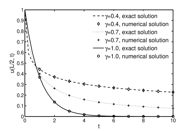
Figure 1: The diffusion curves of time-fractional diffusion model (58) at $x=L/2$, obtained by the quadratic element. Nodal spacing $h=L/100$ and space size $L=10$.

If the diffusion coefficient $k=L^{2}/\pi^{2}$, the exact solution is $u_{exact}(x,t)=sin(\pi x/L)E_{\gamma}(-t^{\gamma})$ whose value at $x=L/2$ is shown in Figure 1 for $\gamma=0.4,0.7$ and $1.0$.

To construct the spatial discretization, both linear and quadratic elements are attempted. For the linear element, the shape functions are:

$$\begin{array}[]{c}\displaystyle{N_{1}(\xi)=(1-\xi)/2,\,\,N_{2}(\xi)=(1+\xi)/2,\,\,\xi\in[-1,\,1]},\end{array}$$ (60)

and the element matrices are:

$$\textbf{C}^{e}=\frac{h}{6}\left[\begin{array}[]{cc}2&1\\ 1&2\end{array}\right],\;\textbf{K}^{e}=\frac{k}{h}\left[\begin{array}[]{cc}1&-1\\ -1&1\end{array}\right]\;$$ (65)

in which $h$ is the nodal spacing. For the quadratic element, the shape functions are:

$$\begin{array}[]{c}\displaystyle{N_{1}(\xi)=-\xi(1-\xi)/2,\,\,N_{2}(\xi)=(1-\xi^{2}),\,\,N_{3}(\xi)=\xi(1+\xi)/2},\end{array}$$ (67)

and the corresponding element matrices are:

$$\textbf{C}^{e}=\frac{h}{30}\left[\begin{array}[]{ccc}4&2&-1\\ 2&16&2\\ -1&2&4\end{array}\right],\;\textbf{K}^{e}=\frac{k}{3h}\left[\begin{array}[]{ccc}7&-8&1\\ -8&16&-8\\ 1&-8&7\end{array}\right].\;$$ (74)

Table 1 lists the normalized errors at different time instants yielded by using $10$ linear, $10$ quadratic and $100$ linear elements. The proposed method can achieve accurate results no matter linear or or quadratic elements are employed. As usual, the quadratic element delivers much more accurate results than the linear element at the same nodal spacing. Another important feature of this method is that the accuracy of numerical result at large time constants can be improved by reducing the nodal spacing $h$.

Table 1: A comparison of normalized errors (Error$=|(u_{exact}(L/2,t)-u(L/2,t))/u_{exact}(L/2,t)|$) of the linear element and the quadratic element. Space size $L=10$, time-fractional derivative order $\gamma=0.8$ and diffusion coefficient $k=L^{2}/\pi^{2}$ in (58).

Time	Linear element	Quadratic element	Linear element
	($h=L/10$)	($h=L/10$)	($h=L/100$)
t=0.0	0.00000000	0.00000000	0.00000000
t=0.1	1.3517e-003	1.0525e-006	1.3485e-005
t=0.2	2.2855e-003	0.4709e-006	2.2814e-005
t=0.3	3.0766e-003	1.7646e-006	3.0726e-005
t=0.4	3.7734e-003	2.9057e-006	3.7703e-005
t=0.5	4.3983e-003	3.9302e-006	4.3965e-005
t=0.6	4.9644e-003	4.8592e-006	4.9643e-005
t=0.7	5.4805e-003	5.7070e-006	5.4825e-005
t=0.8	5.9530e-003	6.4838e-006	5.9572e-005
t=0.9	6.3868e-003	7.1975e-006	6.3934e-005

To estimate the convergence ratio of the linear element and the quadratic element, the results in Table 2 evaluated at $t=10$ but different nodal spacings are prepared and the $L_{\infty}$-error is:

$$\begin{array}[]{c}\displaystyle{L_{\infty,h}=\max_{i}|u_{exact}(x(i),t)-u(x(i),t)|,\,\,i=1,2,...,L/h,}\end{array}$$ (76)

It can be seen that the convergence ratio of the linear element is $O(h^{2})$ and the quadratic element is $O(h^{4})$.

In Table 1, the normalized errors increase with $t$. To investigate the efficiency in tackling long-time range diffusion problems, the normalized errors of the linear and the quadratic elements at large $t$ are computed and listed in Table 3. It can be seen that the normalized errors remain fairly steady with respect to $t$.

Table 2: The $L_{\infty}$-errors and convergence ratios of the linear element and the quadratic element ($Ratio=log(L_{\infty,h_{1}}/L_{\infty,h_{2}})[log(h_{1}/h_{2})]^{-1}$) [41]. Time-fractional derivative order $\gamma=0.8$, space size $L=10$, diffusion coefficient $k=L^{2}/\pi^{2}$ and $t=10$ in (58).

Nodal spacing	$L_{\infty}$-error	Ratio	$L_{\infty}$-error	Ratio
	(Linear element)		(Quadratic element)
h=L/10	4.327591e-004		7.739342e-007
h=L/20	1.087320e-004	1.9928	4.909022e-008	3.9787
h=L/40	2.721688e-005	1.9982	3.080541e-009	3.9942
h=L/80	6.806336e-006	1.9996	1.937557e-010	3.9909
h=L/160	1.701717e-006	1.9999	1.265827e-011	3.9361

Table 3: The normalized errors (Error$=|(u_{exact}(L/2,t)-u(L/2,t))/u_{exact}(L/2,t)|$) of the quadratic element. Space size $L=10$, diffusion coefficient $k=L^{2}/\pi^{2}$, node spacing $h=L/100$ and time-fractional derivative order $\gamma=0.8$ in (58).

Methods	t=10	t=100	t=1000	t=10000
Linear element	1.0136e-004	8.4909e-005	8.2652e-005	8.2307e-005
Quadratic element	1.3185e-009	1.0614e-009	1.0242e-009	1.0186e-009

3.2 One dimensional time-fractional convection-dispersion equation

Time-fractional advection-dispersion equation (also called time-fractional Fokker-Planck equation), which exhibits heavy-tail concentration decay feature, is usually used to characterize contaminant transport in natural porous media. A simple example is:

$$\left\{\begin{array}[]{c}\displaystyle{\frac{d^{\gamma}u(x,t)}{dt^{\gamma}}=-a\frac{\partial u(x,t)}{\partial x}+k\frac{\partial^{2}u(x,t)}{\partial x^{2}},\,\,x\in(0,L),\,\,t>0,}\\ \displaystyle{u(0,t)=E_{\gamma}(-(a-k)t^{\gamma}),\,\,\,\,u(L,t)=e^{L}E_{\gamma}(-(a-k)t^{\gamma}),}\\ u(x,0)=e^{x},\,\,x\in[0,L].\end{array}\right.\;$$ (80)

Assuming $a$ and $k$ are constants, $a>k$, the exact solution of above equation can be written as:

$$\displaystyle{u_{exact}(x,t)=e^{x}E_{\gamma}(-(a-k)t^{\gamma})}$$ (81)

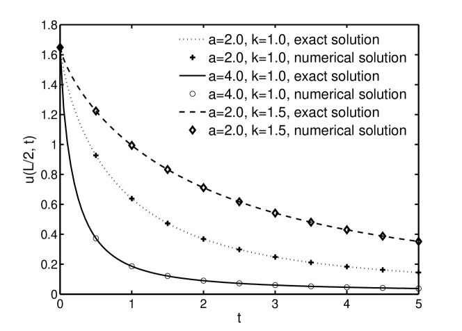
Figure 2: A comparison of exact and numerical solutions of time-fractional advection-dispersion model (80) at $x=L/2$ with $\gamma=0.8$. Nodal spacing $h=L/20$ and space size $L=1.0$ in the linear element.

which is portrayed in Figure 2 for $t<1$. For the linear element, the corresponding element matrices are:

$$\textbf{C}^{e}=\frac{h}{6}\left[\begin{array}[]{cc}2&1\\ 1&2\end{array}\right],\;\textbf{K}^{e}=\frac{a}{2}\left[\begin{array}[]{cc}-1&1\\ -1&1\end{array}\right]\;+\frac{k}{h}\left[\begin{array}[]{cc}1&-1\\ -1&1\end{array}\right].\;$$ (88)

The normalized errors obtained by using $10$, $20$ and $40$ elements at $x=L/2$ and different $t$ are shown in Table 4. With only 10 elements, the errors have been less than $0.1\%$.

3.3 Two dimensional time-fractional diffusion equation

In this example, the following two-dimensional problem is considered:

$$\left\{\begin{array}[]{c}\displaystyle{\frac{d^{\gamma}u(x,y,t)}{dt^{\gamma}}=k(\frac{\partial^{2}u(x,y,t)}{\partial x^{2}}+\frac{\partial^{2}u(x,y,t)}{\partial y^{2}}),\,\,(x,y)\in\Omega,}\\ \displaystyle{u(x,y,t)=0,\,\,(x,y)\in\partial\Omega,\,\,t>0,}\\ u(x,y,0)=sin(x\pi/L)sin(y\pi/L),\,\,(x,y)\in\Omega\cup\partial\Omega,\end{array}\right.\;$$ (92)

in which $k$ is the diffusion coefficient, $\Omega=[0,L]\times[0,L]$. If $k=1/\pi^{2}$ and $L=1.0$, the exact solution of the problem is $u_{exact}(x,y,t)=sin(x\pi)sin(y\pi)E_{\gamma}(-2t^{\gamma})$.

Table 4: The normalized errors (Error$=|(u_{exact}(L/2,t)-u(L/2,t))/u_{exact}(L/2,t)|$) of the linear element. Space size $L=1.0$, diffusion coefficient $k=1.0$,   convective coefficient $a=2.0$ and time-fractional derivative order $\gamma=0.8$ in (80).

Nodal spacing	t=2.0	t=4.0	t=6.0	t=8.0
h=L/10	0.9860e-004	0.9790e-004	0.9724e-004	0.9677e-004
h=L/20	0.2459e-004	0.2441e-004	0.2425e-004	0.2413e-004
h=L/40	0.6143e-005	0.6099e-005	0.6058e-005	0.6029e-005

The square problem domain is modeled by $4\times 4$, $8\times 8$ and $16\times 16$ four-node square elements. The element interpolation functions are:

$$\begin{array}[]{c}\displaystyle{N_{1}=(1-\xi)(1-\eta)/4,\,\,N_{2}=(1+\xi)(1-\eta)/4,}\\ \displaystyle{N_{3}=(1+\xi)(1+\eta)/4,\,\,N_{4}=(1-\xi)(1+\eta)/4,\,\,\xi,\eta\in[-1,\,1]}\end{array}$$ (95)

and

$$\textbf{C}^{e}=\frac{h^{2}}{36}\left[\begin{array}[]{cccc}4&2&1&2\\ 2&4&2&1\\ 1&2&4&2\\ 2&1&2&4\\ \end{array}\right],\;\textbf{K}^{e}=\frac{k}{6}\left[\begin{array}[]{cccc}4&-1&-2&-1\\ -1&4&-1&-2\\ -2&-1&4&-1\\ -1&-2&-1&4\\ \end{array}\right].\;$$ (104)

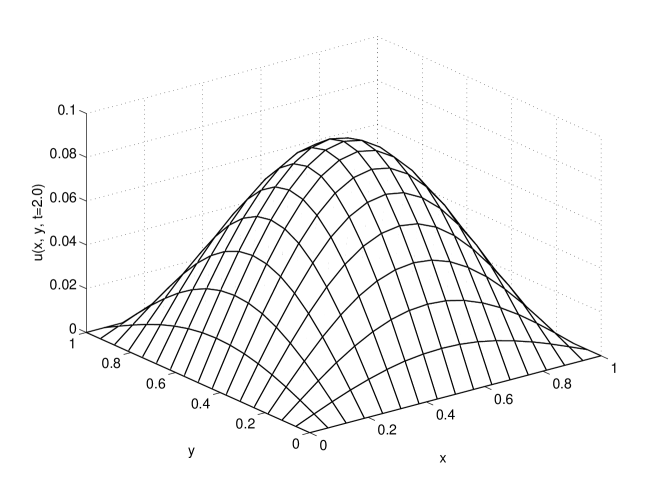
Figure 3: The numerical result of two dimensional time-fractional diffusion model (92) with $\gamma=0.8$ at $t=2.0$. Diffusion coefficient $k=1/\pi^{2}$, space sizes $L=1.0$ and nodal spacing $h=L/16$.

Following the calculation steps (47)-(53), Figure 3 plots the numerical solution for $\gamma=0.8$ at $t=2$, the normalized errors for $\gamma=0.8$ at $x=L/2$, $y=L/2$ and various values of $t$ are given in Table 5. The errors drop with the nodal spacings. Indeed, the finite element method can readily take coordinate-dependent and direction-dependent diffusion coefficients into account.

Table 5: The normalized errors (Error$=|(u_{exact}(L/2,L/2,t)-u(L/2,L/2,t))/u_{exact}(L/2,L/2,t)|$) of the four-node square element. Space size $L=1.0$, nodal spacings $h=h_{x}=h_{y}$, diffusion coefficient $k=1/\pi^{2}$ and time-fractional derivative order $\gamma=0.8$ in (92).

Space step	t=2.0	t=4.0	t=6.0	t=8.0
h=L/4	6.5673e-002	6.1143e-002	5.7924e-002	5.6111e-002
h=L/8	1.6937e-002	1.5786e-002	1.4929e-002	1.4444e-002
h=L/16	4.2664e-003	3.9778e-003	3.7602e-003	3.6368e-003

3.4 Time-fractional diffusion equation in a quarter of circular domain

An important advantage of the finite element method over the finite difference method is that the former can readily consider complex spatial domains. In this example, the following problem defined over a circular domain is considered:

$$\left\{\begin{array}[]{c}\displaystyle{\frac{d^{\gamma}u(x,y,t)}{dt^{\gamma}}=k(\frac{\partial^{2}u(x,y,t)}{\partial x^{2}}+\frac{\partial^{2}u(x,y,t)}{\partial y^{2}}),\,\,(x,y)\in\Omega,}\\ \displaystyle{\textbf{n}^{T}(\textbf{D}\nabla u)=0,\,\,x=0,\,y\neq 1,\,\,\text{and}\,\,y=0,\,0<x<1,\,\,t>0},\\ \displaystyle{u(x,y,t)=J_{0}(1)E_{\gamma}(-t^{\gamma}),\,\,(x,y)\in\{(x,y)|x^{2}+y^{2}=1\}},\\ \displaystyle{u(x,y,0)=J_{0}(\sqrt{x^{2}+y^{2}})},\,\,(x,y)\in\Omega\cup\partial\Omega\end{array}\right.\;$$ (109)

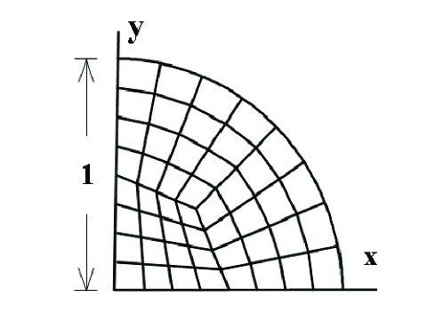
Figure 4: The quadrant of a circle domain with unit radius meshed into 48 elements.

in which $\Omega=\{(x,y)|x>0,\,\,y>0,\,\,x^{2}+y^{2}<1\}$. If $k=1$, the exact solution of (109) is $u_{exact}(x,y,t)=J_{0}(\sqrt{x^{2}+y^{2}})E_{\gamma}(-t^{\gamma})$, in which $J_{0}$ represents the zeroth order Bessel function of the first kind. For symmetry, we only need to model a quarter of the problem domain and a typical mesh is depicted in Figure 4.

For the four-node element, the $(x,y)$ coordinates are also interpolated with the functions given in (95), i.e.

$$\begin{array}[]{c}\displaystyle{x^{e}(\xi,\eta)=\sum_{i=1}^{4}N_{i}x_{i}^{e},\,\,y^{e}(\xi,\eta)=\sum_{i=1}^{4}N_{i}y_{i}^{e}}\\ \end{array}$$ (111)

in which ($x_{i}^{e},\,y_{i}^{e}$) are the coordinates of the $i$-th element nodes.

$$\left\{\begin{array}[]{c}\displaystyle{\textbf{C}^{e}=\int_{-1}^{1}\int_{-1}^{1}(\textbf{N}^{e})^{T}\textbf{N}^{e}det(\textbf{J})d\xi d\eta,}\\ \displaystyle{\textbf{K}^{e}=\int_{-1}^{1}\int_{-1}^{1}(\nabla\textbf{N}^{e})^{T}\textbf{J}^{-1}\textbf{D}\textbf{J}^{-T}(\nabla\textbf{N}^{e})det(\textbf{J})d\xi d\eta}.\end{array}\right.\;$$ (114)

In the above expression,

$$\nabla=\left\{\begin{array}[]{c}\partial/\partial\xi\\ \partial/\partial\eta\end{array}\right\}\;\text{and}\,\,\,\,\textbf{J}=\left[\begin{array}[]{cc}\partial x^{e}/\partial\xi&\partial y^{e}/\partial\xi\\ \partial x^{e}/\partial\eta&\partial y^{e}/\partial\eta\end{array}\right].\;$$ (119)

The matrices $C^{e}$ and $K^{e}$ are computed by the second order Gauss-Legendre rule. In our computations, a quarter circle is partitioned into 3, 48 and 217 elements, the corresponding numerical results at some selected spatial locations are listed in Table 6 for $\gamma=0.8$. Table 6 indicates that the proposed method is capable of delivering accurate solution to anomalous diffusion problem (109) and the accuracy can be improved by employing more elements in modeling the computational domain.

Table 6: The numerical results by different numbers of elements, In the computation, $k(x)=k(y)=1$, the exact solution of (92) is $u_{exact}(x,y,t)=J_{0}(\sqrt{x^{2}+y^{2}})E_{\gamma}(-t^{\gamma}),\,\,\gamma=0.8$.

Coordinates	3 Elements	48 Elements	217 Elements	Exact solution
(0,0)	0.37770	0.38638	0.38681	0.38695
(0.35355, 0.35355)	0.34055	0.36233	0.36292	0.36314
(0.21339, 0.21339)	—	0.37760	0.37804	0.37819
(0.42678, 0.17678)	—	0.36603	0.36644	0.36658
(0.67533, 0.27973)	—	0.33659	0.33687	0.33696
(0.53033, 0.53033)	—	0.33404	0.33432	0.33442
(0.27973, 0.67533)	—	0.33659	0.33687	0.33696
(0.17678, 0.42678)	—	0.36603	0.36644	0.36658

4 Application

To investigate the efficiency and applicability of the proposed semi-analytical method in solving real-world problems, it is employed to solve the problem of tracer solute transport in an aquifer. The experiment was conducted using a test aquifer in Nevada and the schematic diagram is shown in Figure 5 [13]. Bromide of quantity $M=20.81$ kg was used as a nonsorbing tracer solute and introduced to the injection well for a period of $T_{0}=3.54$ days at an average concentration of $3.77$ kg/m³. A reference point, the injection well and extraction well are located at $r=0$ m , 30 m ($R_{i}$) and 60 m ($R_{e}$) along the downstream direction of the underground water flow. The radius of the extraction well is $0.127$ m, the center of extraction well is at $r_{c}=60.127$ m, the pumping rate is $Q=12.4$ m³/d. The solute concentration in the extraction well had been monitored for about 321 days and the screened interval was $b=35$ m . More detailed description of the experiment can be found in [13, 42, 43, 44, 45].

Since $T_{0}$ is short compared with the total time range ($\sim$ 321 days) of measurement, the following radial initial-boundary value problem for the solute transport in the fractured granite aquifer is established in terms of the solute concentration $u$ as:

$$\left\{\begin{array}[]{c}\displaystyle{\frac{d^{\gamma}u(r,t)}{dt^{\gamma}}=-\frac{\upsilon_{0}}{r_{c}-r}\frac{\partial u(r,t)}{\partial r}+\frac{1}{r_{c}-r}\frac{\partial}{\partial r}(d_{0}\frac{\partial u(r,t)}{\partial r}),\,\,r\in(0,R_{e}),}\\ \displaystyle{u(0,t)=0,\,\,\,\,\frac{\partial u(R_{e},t)}{\partial r}=0,\,\,t>0,}\\ u(r,0)=f(r),\,\,r\in[0,R_{e}]\end{array}\right.\;$$ (123)

where $\upsilon_{0}$ is the convective coefficient, $d_{0}$ is the dispersion coefficient, $\upsilon_{0}=ad_{0}$ and $a$ is the dispersivity. Moreover $\upsilon_{0}/(r_{c}-r)$ and $d_{0}/(r_{c}-r)$ have the units of $[L/T^{\gamma}]$ and $[L^{2}/T^{\gamma}]$ which represent the nonlocal aquifer properties [3]. The initial value is normalized as $f(r)=M\delta(r-(r_{c}-R_{i}))/(2\pi(r_{c}-R_{i})b\theta T_{0})$, $\theta$ is the hydraulic parameter. The boundary conditions imply that the solute cannot reach $r=0$ by upstream dispersion and the solute moves by advection at $r=R_{e}$ which gives the wall of the extraction well [13].

In order to obtain a high accurate numerical approximation, the quadratic element is adopted, the element matrices $C^{e}$ and $K^{e}$ are computed by the second order Gauss-Legendre rule.

A comparison of the numerical predictions and the experimental data is shown in Figure 6 and the heavy-tail feature characterized by the time-fractional model (123) with different derivative orders is shown in Figure 7. It can be observed from Figure 6 that the numerical result offers a good fit to most of the experimental data. Due to the subdiffusion behavior in the aquifer matrix and immobile water, in the experimental result, the concentration of bromide exhibits a rather slow decay in the late time. Figure 7 confirms that the time-fractional radial flow model (123) captures the long-time behavior with heavy-tail. Figure 7 also illustrates that the heavy-tail feature becomes more remarkable with the decreasing of the time-fractional derivative order $\gamma$. Hence, in this model (123), the time-fractional derivative order $\gamma$ is a indicator of the non-Fickian transport caused by the complex structure of the fractured aquifer.

5 Discussions

By using the finite element to discretize the spatial domain, the fractional diffusion equations can be reduced to approximate fractional relaxation equations which possess analytical solutions. The semi-analytical method can not only compute time-fractional diffusion equations in long-time range at low computational cost but also deliver accurate numerical predictions for complex and large spatial problem domains. The accuracy in spatial domain can be improved by using more elements, high-order elements or elements based on advanced finite element formulations. Since the exact solution is used in time domain, the stability and convergence conditions of the proposed method can be easily satisfied. It can be said that the proposed method is more robust than previous ones.

The main restriction for the proposed method is that the weak forms of time diffusion equations can be transformed into the following form:

$$\begin{array}[]{c}\displaystyle{\textbf{C}\frac{d^{\gamma}}{dt^{\gamma}}\textbf{u}+\textbf{K}\textbf{u}=0}.\end{array}$$ (125)

In cases that the source term, physical parameters and/or boundary conditions are only weak function(s) of time, a multiple time step method can be used.

6 Concluding remarks

From formulations and examples presented, it is clear that a class of time-fractional diffusion equations can be easily computed and the heavy-tail feature can be accurately characterized by the new method. Our future research work will focus on advanced finite element formulations, such as hybrid element [46], to compute temporal-spatial fractional diffusion equations which characterize more complex contaminant transport problems.

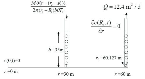
Figure 5: A schematic diagram of experiment.

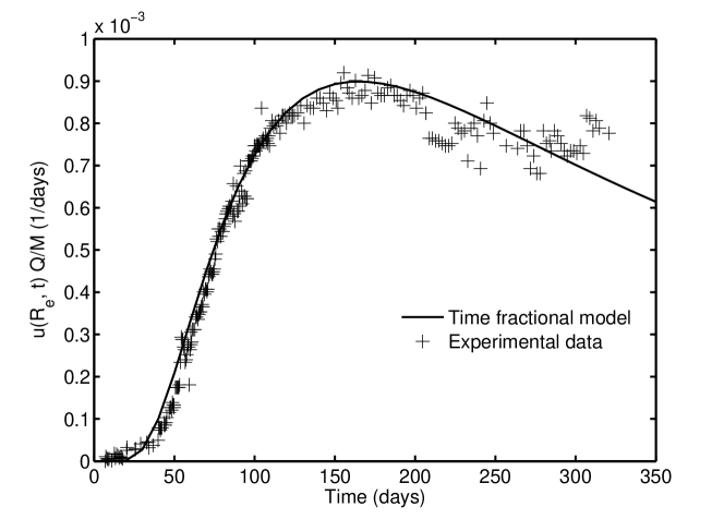
Figure 6: The numerical approximation of the time-fractional radial flow advection-dispersion equation model (109) with $\gamma=0.92$ at $r=R_{e}$. In this numerical simulation, convective coefficient $\upsilon_{0}=0.0564/\theta,\,\,\theta=0.023$, the dispersion coefficient $d_{0}=a\upsilon_{0},\,\,a=6.8$, nodal spacing $h=3$ and time step is $\Delta t=10$.

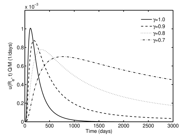
Figure 7: The numerical approximation of the time-fractional radial flow advection-dispersion equation model (109) with different time-fractional derivative values $\gamma$ at $r=R_{e}$. In this numerical simulation, convective coefficient $\upsilon_{0}=0.0564/\theta,\,\,\theta=0.023$, dispersion coefficient $d_{0}=a\upsilon_{0},\,\,a=6.8$, nodal spacing $h=3$ and time step is $\Delta t=10$. The curve with $\gamma=1.0$ corresponding to Fickian dispersion.

References

- [1] G. Dagan. Theory of solute transport by groundwater. Ann Rev Fluid Mech 1987; 19: 183-215.
- [2] E. M. LaBolle, G. E. Fogg. Role of molecular diffusion in contaminant migration and recovery in an alluvial aquifer system. Transport Porous Med 2001; 42: 155-179.
- [3] Y. Zhang, D. A. Benson, D. M. Reeves. Time and space nonlocalities underlying fractional-derivative models: Distinction and literature review of field applications. Adv Water Resour 2009; 32: 561-581.
- [4] R. Metzler, J. Klafter. The random walk’s guide to anomalous diffusion: a fractional dynamics approach. Phys Rep 2000; 339: 1-77.
- [5] Q. Z. Huang, G. H. Huang, H. B. Zhan. A finite element solution for the fractional advection-dispersion equation. Adv Water Resour 2008; 31: 1578-1589.
- [6] B. Berkowitz, A. Cortis, M. Dentz, H. Scher. Modeling non-Fickian transport in geological formations as a continuous time random walk. Rev Geophys 2006; 44(2): RG2003.
- [7] B. Berkowitz, H. Scher. On characterization of anomalous dispersion in porous media. Water Resour Res 1995; 31: 1461-1466.
- [8] X. X. Zhang, M. Lv, J. W. Crawford, I. M. Young. The impact of boundary on the fractional advection Cdispersion equation for solute transport in soil: Defining the fractional dispersive flux with the Caputo derivatives. Adv Water Resour 2007; 30: 1205-1217.
- [9] H. G. Sun, W. Chen, Y. Q. Chen. Variable-order fractional differential operator in anomalous diffusion modeling. Phys A 2009; 388: 4586-4592.
- [10] D. A. Benson, S. W. Wheatcraft, M. M. Meerschaert. Application of a fractional advection-dispersion equation. Water Resour Res 2000; 36(6): 1403-1412.
- [11] J. D. Seymour, J. P. Gage, S. L. Codd, R. Gerlach. Magnetic resonance microscopy of biofouling induced scale dependent transport in porous media. Adv Water Resour 2007; 30(6-7): 1408-1420.
- [12] M. M. Meerschaert, D. A. Benson, B. Baeumer. Operator Lvy motion and multiscaling anomalous diffusion. Phys Rev E 2001; 63: 021112.
- [13] D. A. Benson, C. Tadjeran, M. M. Meerschaert, I. Farnham, G. Pohll. Radial fractional-order dispersion through fractured rock. Water Resour Res 2004; 40: W12416.
- [14] I. M. Sokolov, J. Klafter. From diffusion to anomalous diffusion: A century after Einstein’s Brownian motion. Chaos 2005; 15: 026103.
- [15] G. M. Zaslavsky. Chaos, fractional kinetics, and anomalous transport. Phys Rep 2002; 371 (6): 461-580.
- [16] R. L. Magin, O. Abdullah, D. Baleanu, et al. Anomalous diffusion expressed through fractional order differential operators in the Bloch-Torrey equation. J Magn Reson 2008; 190 (2): 255-270.
- [17] I. Podlubny, A. Chechkin, T. Skovranek, Y. Q. Chen, B. M. Vinagre Jara. Matrix approach to discrete fractional calculus II: Partial fractional differential equations. J Comput Phys 2009; 228: 3137-3153.
- [18] J. P. Roop. Computational aspects of FEM approximation of fractional advection dispersion equations on bounded domains in . J Comput Appl Math 2006; 193: 243-268.
- [19] C. Li, A. Chen, J. J. Ye. Numerical approaches to fractional calculus and fractional ordinary differential equation. J Comput Phys 2011; 230(9): 3352-3368.
- [20] I. Podlubny. Fractional differential equation. San Diego, Academic press, 1999. 50-78.
- [21] N. J. Ford, A. C. Simpson. The numerical solution of fractional differential equations: speed versus accuracy. Numer Algorithms 2001; 26: 336-346.
- [22] F. A. Radu, N. Suciu, J. Hoffmann, A. Vogel, O. Kolditz, C. H. Park, S. Attinger. Accuracy of numerical simulations of contaminant transport in heterogeneous aquifers: A comparative study. Adv Water Resour 2011; 34: 47-61.
- [23] O. C. Zienkiewicz, R. L. Taylor. The finite element method: Volume 3 Fluid Dynamics fifth edition. Oxford, Butterworth-Heinemann, 2000.
- [24] R. W. Lewis, K. Morgan, H. R. Thomas, K. N. Seetharamu. The finite element method in heat transfer analysis. New York, John Wiley & Sons, 1996.
- [25] J. M. Bergheau, R. Fortunier. Finite element simulation of heat transfer. London, John Wiley & Sons, 2008.
- [26] I. M. Smith, D. V. Griffiths. Programming the finite element method (4th edition) . New York, John Wiley & Sons Ltd, 2004.
- [27] S. B. Yuste. Weighted average finite difference methods for fractional diffusion equations. J Comput Phys 2006; 216: 264-274.
- [28] C. M. Chen, F. Liu, I. Turner, V. Anh. A Fourier method for the fractional diffusion equation describing sub-diffusion. J Comput Phys 2007; 227: 886-897.
- [29] G. J. Fix, J. P. Roop. Least squares finite-element solution of a fractional order two-point boundary value problem. Comput & Math Appl 2004; 48 (7-8): 1017-1033.
- [30] W. H. Deng. Finte element method for the space and time fractional Fokker-Planck equation. SIAM J Numer Anal 2008; 47(1):204-226.
- [31] H. Zhang, F. Liu, V. Anh. Galerkin finite element approximation of symmetric space-fractional partial differential equations. Appl Math Comput 2010; 217(6):2534-2545.
- [32] Y. Y. Zheng, C. P. Li, Z. G. Zhao. A note on the finite element method for the space-fractional advection diffusion equation. Comput & Math Appl 2010; 59: 1718-1726.
- [33] Y. Y. Zheng, C. P. Li, Z. G. Zhao. A fully discrete discontinuous Galerkin method for nonlinear fractional Fokker-Planck equation. Math Probl Engng 2010; doi:10.1155/2010/279038.
- [34] C. P. Li, Z. G. Zhao, Y. Q. Chen. Numerical approximation of nonlinear fractional differential equuations with subdiffusion and superdiffusion. Comput & Math Appl 2011; doi:10.1016/j.camwa.2011.02.045.
- [35] S. G. Samko, A. A. Kilbas, O. I. Marichev. Fractional integrals and derivatives: theory and applications. Gordon and Breach, Taylor & Francis Ltd, 1993.
- [36] P. Kumar, O. P. Agrawal. An approximate method for numerical solution of fractional differential equations. Signal Processing 2006; 86 (10), 2602-2610.
- [37] G. L. Guymon. A finite element solution of the one-dimensional diffusion-convection equation. Water Resour Res 1970; 6(1): 204-210.
- [38] F. Mainardi. Fractional relaxation-oscillation and fractional diffusion-wave phenomena. Chaos, Solitons & Fractals 1996; 7(9): 1461-1477.
- [39] I. Podlubny. Mittag-Leffler function. http://www.mathworks.de /matlabcentral/fileexchange/8738-mittag-leffler-function 2009.
- [40] Y. Q. Chen. Generalized Mittag-Leffler function. http://www.mathworks.de/matlabcentral/fileexchange/20849-generalized-mittag-leffler-function 2008.
- [41] L. J. Su, W. Q. Wang, Z. X. Yang. Finite difference approximations for the fractional advection-diffusion equation. Phys Lett A 2009; 373: 4405-4408.
- [42] M. M. Meerschaert, C. Tadjeran. Finite difference approximations for fractional advection-dispersion flow equations. J Comput Appl Math 2004; 172: 65-77.
- [43] P. Reimus, G. Pohll, T. Mihevc, J. Chapman, M. Haga, B. Lyles, S. Kosinski, R. Niswonger, P. Sanders. Testing and parameterizing a conceptual model for solute transport in a fractured granite using multiple tracers in a forced-gradient test. Water Resour Res 2003; 39: 1356-1370.
- [44] G. Pohll, A. E. Hassan, J. B. Chapman, C. Papelis, R. Andricevic. Modeling ground water flow and radioactive transport in a fractured aquifer. Ground Water 1999; 37(5): 770-784.
- [45] P. W. Reimus, M. J. Haga, A. I. Adams, T. J. Callahan, H. J. Turin, D. A. Coun. Testing and parameterizing a conceptual solute transport model in saturated fractured tuff using sorbing and nonsorbing tracers in cross-hole tracer tests. J Contam Hydrol 2003; 62-63: 613-636.
- [46] K. Y. Sze, Y. K. Cheung. A hybrid-Trefftz finite element model for Helmholtz problem. Commun Numer Meth Engng 2008; 24: 2047-2060.