A Mean-Reverting SDE on Correlation Matrices

Abstract

We introduce a mean-reverting SDE whose solution is naturally defined on the space of correlation matrices. This SDE can be seen as an extension of the well-known Wright-Fisher diffusion. We provide conditions that ensure weak and strong uniqueness of the SDE, and describe its ergodic limit. We also shed light on a useful connection with Wishart processes that makes understand how we get the full SDE. Then, we focus on the simulation of this diffusion and present discretization schemes that achieve a second-order weak convergence. Last, we explain how these correlation processes could be used to model the dependence between financial assets.

Key words: Correlation, Wright-Fisher diffusions, Multi-allele Wright-Fisher model, Jacobi processes, Wishart processes, Discretization schemes, Multi-asset model.

AMS Class 2010: 65C30, 60H35, 91B70.

Acknowledgements: We would like to acknowledge the support of the Credinext project from Finance Innovation, the “Chaire Risques Financiers” of Fondation du Risque and the French National Research Agency (ANR) program BigMC.

Introduction

The scope of this paper is to introduce an SDE that is well defined on the set of correlation matrices. Our main motivation comes from an application to finance, where the correlation is commonly used to describe the dependence between assets. More precisely, a diffusion on correlation matrices can be used to model the instantaneous correlation between the log-prices of different stocks. Thus, it is also very important for practical purpose to be able to sample paths of this SDE in order to compute expectations (for prices or greeks). This is why an entire part of this paper is devoted to get an efficient simulation scheme. More generally, processes on correlation matrices can naturally be used to model the dynamics of the dependence between some quantities and can be applied to a much wider range of applications. In this paper, we mainly focus on the definition, the mathematical properties and the sampling of this SDE. However, we discuss in Section 4 a possible implementation of these processes in finance to model a basket of risky assets.

There are works on particular Stochastic Differential Equations that are defined on positive semidefinite matrices such as Wishart processes (Bru [5]) or their Affine extensions (Cuchiero et al. [8]). On the contrary, there is to the best of our knowledge very few literature dedicated to some stochastic differential equations that are valued on correlation matrices. Of course, general results are known for stochastic differential equations on manifolds. However, no particular SDE defined on correlation matrices has been studied in detail. In dimension $d=2$, correlation matrices are naturally described by a single real $\rho\in[-1,1]$. The probably most famous SDE on $[-1,1]$ is the following Wright-Fisher diffusion:

$$dX_{t}=\kappa(\bar{\rho}-X_{t})dt+\sigma\sqrt{1-X_{t}^{2}}dB_{t},$$ (1)

where $\kappa\geq 0,\ \bar{\rho}\in[-1,1],\ \sigma\geq 0$, and $(B_{t})_{t\geq 0}$ is a real Brownian motion. Here, we make a slight abuse of language. Strictly speaking, Wright-Fisher diffusions are defined on $[0,1]$ and this is in fact the process $(\frac{1+X_{t}}{2},t\geq 0)$ that is a Wright-Fisher one. They have originally been used to model gene frequencies (see Karlin and Taylor [20]). The marginal law of $X_{t}$ is known explicitly with its moments, and its density can be written as an expansion with respect to the Jacobi orthogonal polynomial basis (see Mazet [23]). This is why the process $(X_{t},t\geq 0)$ is sometimes also called Jacobi process in the literature. In higher dimension ($d\geq 3$), no similar SDE has been yet considered. To get processes on correlation matrices, it is instead used parametrization of subsets of correlation matrices. For example, one can consider $X_{t}$ defined by $(X_{t})_{i,j}=\rho_{t}$ for $1\leq i\not=j\leq d$, where $\rho_{t}$ is a Wright-Fisher diffusion on $[-1/(d-1),1]$. More sophisticated examples can be found in [21]. The main purpose of this paper is to propose a natural extension of the Wright-Fisher process (1) that is defined on the whole set of correlation matrices.

Let us now introduce the process. We first advise the reader to have a look at our notations for matrices located at the end if this introduction, even though they are rather standard. We consider $(W_{t},t\geq 0)$, a $d$-by-$d$ square matrix process whose elements are independent real standard Brownian motions, and focus on the following SDE on the correlation matrices ${\mathfrak{C}_{d}(\mathbb{R})}$:

$$X_{t}=x+\int_{0}^{t}\left(\kappa(c-X_{s})+(c-X_{s})\kappa\right)ds+\sum_{n=1}^{d}a_{n}\int_{0}^{t}\left(\sqrt{X_{s}-X_{s}e_{d}^{n}X_{s}}dW_{s}e_{d}^{n}+e_{d}^{n}dW_{s}^{T}\sqrt{X_{s}-X_{s}e_{d}^{n}X_{s}}\right),$$ (2)

where $x,c\in{\mathfrak{C}_{d}(\mathbb{R})}$ and $\kappa=diag(\kappa_{1},\dots,\kappa_{d})$ and $a=diag(a_{1},\dots,a_{d})$ are nonnegative diagonal matrices such that

$$\kappa c+c\kappa-(d-2)a^{2}\in{\mathcal{S}_{d}^{+}(\mathbb{R})}\text{ or }d=2.$$ (3)

Under these assumptions, we will show in Section 2 that this SDE has a unique weak solution which is well-defined on correlation matrices, i.e. $\forall t\geq 0,X_{t}\in{\mathfrak{C}_{d}(\mathbb{R})}$. We will also show that strong uniqueness holds if we assume moreover that $x\in{\mathfrak{C}_{d}^{*}(\mathbb{R})}$ and

$$\kappa c+c\kappa-da^{2}\in{\mathcal{S}_{d}^{+}(\mathbb{R})}.$$ (4)

Looking at the diagonal coefficients, conditions (3) and (4) imply respectively $\kappa_{i}\geq(d-2)a_{i}^{2}/2$ and $\kappa_{i}\geq da_{i}^{2}/2$. This heuristically means that the speed of the mean-reversion has to be high enough with respect to the noise in order to stay in ${\mathfrak{C}_{d}(\mathbb{R})}$. Throughout the paper, we will denote $MRC_{d}(x,\kappa,c,a)$ the law of the process $(X_{t})_{t\geq 0}$ and ${MRC}_{d}(x,\kappa,c,a;t)$ the law of $X_{t}$. Here, $MRC$ stands for Mean-Reverting Correlation process. When using these notations, we implicitly assume that (3) holds.

In dimension $d=2$, the only non trivial component is $(X_{t})_{1,2}$. We can show easily that there is a real Brownian motion $(B_{t},t\geq 0)$ such that

$$d(X_{t})_{1,2}=(\kappa_{1}+\kappa_{2})(c_{1,2}-(X_{t})_{1,2})dt+\sqrt{a_{1}^{2}+a_{2}^{2}}\sqrt{1-(X_{t})_{1,2}^{2}}dB_{t}.$$

Thus, the process (2) is simply a Wright-Fisher diffusion. Our parametrization is however redundant in dimension $2$, and we can assume without loss of generality that $\kappa_{1}=\kappa_{2}$ and $a_{1}=a_{2}$. Then, the condition $\kappa c+c\kappa\in{\mathcal{S}_{d}^{+}(\mathbb{R})}$ is always satisfied, while assumption (4) is the condition that ensures $\forall t\geq 0,(X_{t})_{1,2}\in(-1,1)$. In larger dimensions $d\geq 3$, we can also show that each non-diagonal element of (2) follows a Wright-Fisher diffusion (1).

The paper is structured as follows. In the first section, we present first properties of Mean-Reverting Correlation processes. We calculate the infinitesimal generator and give explicitly their moments. In particular, this enables us to describe the ergodic limit. We also present a connection with Wishart processes that clarifies how we get the SDE (2). It is also useful later in the paper to construct discretization schemes. Last, we show a link between some MRC processes and the multi-allele Wright-Fisher model. Then, Section 2 is devoted to the study of the weak existence and strong uniqueness of the SDE (2). We discuss the extension of these results to time and space dependent coefficients $\kappa,\ c,\ a$. Also, we exhibit a change of probability that preserves the family of MRC processes. The third section is devoted to obtain discretization schemes for (2). This is a crucial issue if one wants to use MRC processes effectively. To do so, we use a remarkable splitting of the infinitesimal generator as well as standard composition technique. Thus, we construct discretization schemes with a weak error of order $2$. This can be done either by reusing the second order schemes for Wishart processes obtained in [2] or by an ad-hoc splitting (see Appendix D). All these schemes are tested numerically and compared with a (corrected) Euler-Maruyama scheme. In the last section, we explain how Mean-Reverting Correlation processes and possible extensions could be used for the modeling of $d$ risky assets. First, we recall the main advantages of modeling the instantaneous correlation instead of the instantaneous covariance of the assets. Then, we discuss our model and its relevance on index option market data.

Notations for real matrices :

• For $d\in\mathbb{N}^{*}$, $\mathcal{M}_{d}(\mathbb{R})$ denotes the real $d$ square matrices; $\mathcal{S}_{d}(\mathbb{R})$, $\mathcal{S}_{d}^{+}(\mathbb{R}),\mathcal{S}_{d}^{+,*}(\mathbb{R})$, and $\mathcal{G}_{d}(\mathbb{R})$ denote respectively the set of symmetric, symmetric positive semidefinite, symmetric positive definite and non singular matrices.

• The set of correlation matrices is denoted by ${\mathfrak{C}_{d}(\mathbb{R})}$:

  $${\mathfrak{C}_{d}(\mathbb{R})}=\left\{x\in{\mathcal{S}_{d}^{+}(\mathbb{R})},\forall 1\leq i\leq d,\,\,x_{i,i}=1\right\}$$

  We also define ${\mathfrak{C}_{d}^{*}(\mathbb{R})}={\mathfrak{C}_{d}(\mathbb{R})}\cap\mathcal{G}_{d}(\mathbb{R})$, the set of the invertible correlation matrices.

• For $x\in\mathcal{M}_{d}(\mathbb{R})$, $x^{T}$, $\textup{adj}(x)$, $\det(x)$, $\textup{Tr}(x)$ and $\textup{Rk}(x)$ are respectively the transpose, the adjugate, the determinant, the trace and the rank of $x$.

• For $x\in\mathcal{S}_{d}^{+}(\mathbb{R})$, $\sqrt{x}$ denotes the unique symmetric positive semidefinite matrix such that $(\sqrt{x})^{2}=x$

• The identity matrix is denoted by $I_{d}$. We set for $1\leq i,j\leq d$, $e^{i,j}_{d}=(\mathbbm{1}_{k=i,l=j})_{1\leq k,l\leq d}$ and $e^{i}_{d}=e^{i,i}_{d}$. Last, we define $e^{\{i,j\}}_{d}=e^{i,j}_{d}+\mathbbm{1}_{i\not=j}e^{j,i}_{d}$.

• For $x\in{\mathcal{S}_{d}(\mathbb{R})}$, we denote by $x_{\{i,j\}}$ the value of $x_{i,j}$, so that $x=\sum_{1\leq i\leq j\leq d}x_{\{i,j\}}e^{\{i,j\}}_{d}$. We use both notations in the paper: notation $(x_{i,j})_{1\leq i,j\leq d}$ is of course more convenient for matrix calculations while $(x_{\{i,j\}})_{1\leq i\leq j\leq d}$ is preferred to emphasize that we work on symmetric matrices and that we have $x_{i,j}=x_{j,i}$.

• For $\lambda_{1},\dots,\lambda_{d}\in\mathbb{R}$, $diag(\lambda_{1},\dots,\lambda_{d})\in{\mathcal{S}_{d}(\mathbb{R})}$ denotes the diagonal matrix such that $diag(\lambda_{1},\dots,\lambda_{d})_{i,i}=\lambda_{i}$.

• For $x\in{\mathcal{S}_{d}^{+}(\mathbb{R})}$ such that $x_{i,i}>0$ for all $1\leq i\leq d$, we define ${\bf p}(x)\in{\mathfrak{C}_{d}(\mathbb{R})}$ by

  $$({\bf p}(x))_{i,j}=\frac{x_{i,j}}{\sqrt{x_{i,i}x_{j,j}}},\ 1\leq i,j\leq d.$$ (5)

• For $x\in{\mathcal{S}_{d}(\mathbb{R})}$ and $1\leq i\leq d$, we denote by ${x}^{[i]}\in\mathcal{S}_{d-1}(\mathbb{R})$ the matrix defined by ${x}^{[i]}_{k,l}=x_{k+\mathbbm{1}_{k\geq i},l+\mathbbm{1}_{l\geq i}}$ and $x^{i}\in\mathbb{R}^{d-1}$ the vector defined by $x^{i}_{k}=x_{i,k}$ for $1\leq k<i$ and $x^{i}_{k}=x_{i,k+1}$ for $i\leq k\leq d-1$. For $x\in{\mathfrak{C}_{d}(\mathbb{R})}$, we have ${(x-xe^{i}_{d}x)}^{[i]}={x}^{[i]}-x^{i}(x^{i})^{T}$.

1 Some properties of MRC processes

1.1 The infinitesimal generator

We first calculate the quadratic covariation of $MRC_{d}(x,\kappa,c,a)$. By Lemma 27, we get:

$$\langle d(X_{t})_{i,j},d(X_{t})_{k,l}\rangle = \Big{[}a_{i}^{2}(\mathbbm{1}_{i=k}(X_{t}-X_{t}e_{d}^{i}X_{t})_{j,l}+\mathbbm{1}_{i=l}(X_{t}-X_{t}e_{d}^{i}X_{t})_{j,k})$$

$$+a_{j}^{2}(\mathbbm{1}_{j=k}(X_{t}-X_{t}e_{d}^{j}X_{t})_{i,l}+\mathbbm{1}_{j=l}(X_{t}-X_{t}e_{d}^{j}X_{t})_{i,k})\Big{]}dt$$

$$= \Big{[}a_{i}^{2}(\mathbbm{1}_{i=k}((X_{t})_{j,l}-(X_{t})_{i,j}(X_{t})_{i,l})+\mathbbm{1}_{i=l}((X_{t})_{j,k}-(X_{t})_{i,j}(X_{t})_{i,k}))$$

$$+a_{j}^{2}(\mathbbm{1}_{j=k}((X_{t})_{i,l}-(X_{t})_{j,i}(X_{t})_{j,l})+\mathbbm{1}_{j=l}((X_{t})_{i,k}-(X_{t})_{j,i}(X_{t})_{j,k}))\Big{]}dt.$$

We remark in particular that $d\langle(X_{t})_{i,j},d(X_{t})_{k,l}\rangle=0$ when $i,j,k,l$ are distinct.

We are now in position to calculate the infinitesimal generator of $MRC_{d}(x,\kappa,c,a)$. The infinitesimal generator on ${\mathcal{M}_{d}(\mathbb{R})}$ is defined by:

$$x\in{\mathfrak{C}_{d}(\mathbb{R})},\ L^{\mathcal{M}}f(x)=\lim_{t\rightarrow 0^{+}}\frac{\mathbb{E}[f(X^{x}_{t})]-f(x)}{t}\text{ for }f\in\mathcal{C}^{2}({\mathcal{M}_{d}(\mathbb{R})},\mathbb{R})\text{ with bounded derivatives}.$$

By straightforward calculations, we get from (1.1) that:

$$L^{\mathcal{M}}=\sum_{\begin{subarray}{c}1\leq i,j\leq d\\ j\not=i\end{subarray}}(\kappa_{i}+\kappa_{j})(c_{i,j}-x_{i,j})\partial_{i,j}+\frac{1}{2}\sum_{\begin{subarray}{c}1\leq i,j,k\leq d\\ j\not=i,k\not=i\end{subarray}}a_{i}^{2}(x_{j,k}-x_{i,j}x_{i,k})[\partial_{i,j}\partial_{i,k}+\partial_{i,j}\partial_{k,i}+\partial_{j,i}\partial_{i,k}+\partial_{j,i}\partial_{k,i}].$$

Here, $\partial_{i,j}$ denotes the derivative with respect to the element at the $i^{th}$ line and $j^{th}$ column. We know however that the process that we consider is valued in ${\mathfrak{C}_{d}(\mathbb{R})}\subset{\mathcal{S}_{d}(\mathbb{R})}$. Though it is equivalent, it is often more convenient to work with the infinitesimal generator on ${\mathcal{S}_{d}(\mathbb{R})}$, which is defined by:

$$x\in{\mathfrak{C}_{d}(\mathbb{R})},\ Lf(x)=\lim_{t\rightarrow 0^{+}}\frac{\mathbb{E}[f(X^{x}_{t})]-f(x)}{t}\text{ for }f\in\mathcal{C}^{2}({\mathcal{S}_{d}(\mathbb{R})},\mathbb{R})\text{ with bounded derivatives},$$

since it eliminates redundant coordinates. For $x\in{\mathcal{S}_{d}(\mathbb{R})}$, we denote by $x_{\{i,j\}}=x_{i,j}=x_{j,i}$ the value of the coordinates $(i,j)$ and $(j,i)$, so that $x=\sum_{1\leq i\leq j\leq d}x_{\{i,j\}}(e^{i,j}_{d}+\mathbbm{1}_{i\not=j}e^{j,i}_{d})$. For $f\in\mathcal{C}^{2}({\mathcal{S}_{d}(\mathbb{R})},\mathbb{R})$, $\partial_{\{i,j\}}f$ denotes its derivative with respect to $x_{\{i,j\}}$. For $x\in{\mathcal{M}_{d}(\mathbb{R})}$, we set $\pi(x)=(x+x^{T})/2$. It is such that $\pi(x)=x$ for $x\in{\mathcal{S}_{d}(\mathbb{R})}$, and we have $Lf(x)=L^{\mathcal{M}}f\circ\pi(x).$ By the chain rule, we have for $x\in{\mathcal{S}_{d}(\mathbb{R})}$, $\partial_{i,j}f\circ\pi(x)=(\mathbbm{1}_{i=j}+\frac{1}{2}\mathbbm{1}_{i\neq j})\partial_{\{i,j\}}f(x)$ and we get:

$$L=\sum_{i=1}^{d}\left(\sum_{\begin{subarray}{c}1\leq j\leq d\\ j\not=i\end{subarray}}\kappa_{i}(c_{\{i,j\}}-x_{\{i,j\}})\partial_{\{i,j\}}+\frac{1}{2}\sum_{\begin{subarray}{c}1\leq j,k\leq d\\ j\not=i,k\not=i\end{subarray}}a_{i}^{2}(x_{\{j,k\}}-x_{\{i,j\}}x_{\{i,k\}})\partial_{\{i,j\}}\partial_{\{i,k\}}\right).$$ (7)

Then, we will say that a process $(X_{t},t\geq 0)$ valued in ${\mathfrak{C}_{d}(\mathbb{R})}$ solves the martingale problem of $MRC_{d}(x,\kappa,c,a)$ if for any $n\in\mathbb{N}^{*}$, $0\leq t_{1}\leq\dots\leq t_{n}\leq s\leq t$, $g_{1},\dots,g_{n}\in\mathcal{C}({\mathcal{S}_{d}(\mathbb{R})},\mathbb{R})$, $f\in\mathcal{C}^{2}({\mathcal{S}_{d}(\mathbb{R})},\mathbb{R})$ we have:

$$\mathbb{E}\left[\prod_{i=1}^{n}g_{i}(X_{t_{i}})\left(f(X_{t})-f(X_{s})-\int_{s}^{t}Lf(X_{u})du\right)\right]=0,\text{ and }X_{0}=x$$ (8)

Now, we state simple but interesting properties of mean-reverting correlation processes. Each non-diagonal coefficient follows a Wright-Fisher type diffusion and any principal submatrix is also a mean-reverting correlation process. This result is a direct consequence of the calculus above and the weak uniqueness of the SDE (2) obtained in Corollary 3.

Proposition 1

— Let $(X_{t})_{t\geq 0}\sim MRC_{d}(x,\kappa,c,a)$. For $1\leq i\not=j\leq d$, there is Brownian motion $(\beta^{i,j}_{t},t\geq 0)$ such that

$$d(X_{t})_{i,j}=(\kappa_{i}+\kappa_{j})(c_{i,j}-(X_{t})_{i,j})dt+\sqrt{a_{i}^{2}+a_{j}^{2}}\sqrt{1-(X_{t})_{i,j}^{2}}d\beta^{i,j}_{t}.$$ (9)

Let $I=\{k_{1}<\dots<k_{d^{\prime}}\}\subset\{1,\dots,d\}$ such that $1<d^{\prime}<d$. For $x\in{\mathcal{M}_{d}(\mathbb{R})}$, we define $x^{I}\in\mathcal{M}_{d^{\prime}}(\mathbb{R})$ by $(x^{I})_{i,j}=x_{k_{i},k_{j}}$ for $1\leq i,j\leq d^{\prime}$. We have:

$$(X^{I}_{t})_{t\geq 0}\overset{law}{=}MRC_{d^{\prime}}(x^{I},\kappa^{I},c^{I},a^{I}).$$

1.2 Calculation of moments and the ergodic law

We first introduce some notations that are useful to characterise the general form for moments. For every $x\in{\mathcal{S}_{d}(\mathbb{R})},m\in\mathcal{S}_{d}(\mathbb{N}),$ we set:

$$x^{m}=\prod_{1\leq i\leq j\leq d}x_{\{i,j\}}^{m_{\{i,j\}}}\text{ and }|m|=\sum_{1\leq i\leq j\leq d}m_{\{i,j\}}.$$

A function $f:{\mathcal{S}_{d}(\mathbb{R})}\rightarrow\mathbb{R}$ is a polynomial function of degree smaller than $n\in\mathbb{N}$ if there are real numbers $a_{m}$ such that $f(x)=\sum_{|m|\leq n}a_{m}x^{m}$, and we define the norm of $f$ by $\|f\|_{\mathbb{P}}=\sum_{|m|\leq n}|a_{m}|$.

We want to calculate the moments $\mathbb{E}[X_{t}^{m}]$ of $(X_{t},t\geq 0)\sim MRC_{d}(x,\kappa,c,a)$. Since the diagonal elements are equal to $1$, we will take $m_{\{i,i\}}=0$. Let us also remark that for $i\not=j$ such that $\kappa_{i}=\kappa_{j}=0$, we have from (3) that $a_{i}=a_{j}=0$. Therefore we get $(X_{t})_{i,j}=x_{i,j}$ by (9).

Proposition 2

— Let $m\in\mathcal{S}_{d}(\mathbb{N})$ such that $m_{i,i}=0$ for $1\leq i\leq d$. Let $(X_{t})_{t\geq 0}\sim MRC_{d}(x,\kappa,c,a)$. For $m\in\mathcal{S}_{d}(\mathbb{N})$, $Lx^{m}=-K_{m}x^{m}+f_{m}(x)$, with

$$K_{m}=\sum_{i=1}^{d}\sum_{j=1}^{d}\kappa_{i}m_{\{i,j\}}+\frac{1}{2}\sum_{i=1}^{d}a_{i}^{2}\sum_{j,k=1}^{d}m_{\{i,j\}}m_{\{i,k\}}$$

and

$$f_{m}(x)=\sum_{i=1}^{d}\sum_{j=1}^{d}\kappa_{i}c_{\{i,j\}}m_{\{i,j\}}x^{m-e^{\{i,j\}}_{d}}+\frac{1}{2}\sum_{i=1}^{d}a_{i}^{2}\sum_{j,k=1}^{d}m_{\{i,j\}}m_{\{i,k\}}x^{m-e^{\{i,j\}}_{d}-e^{\{i,k\}}_{d}+e^{\{j,k\}}_{d}}$$

is a polynomial function of degree smaller than $|m|-1$. We have

$$\mathbb{E}\left[X_{t}^{m}\right]=x^{m}\exp(-tK_{m})+\exp(-tK_{m})\int_{0}^{t}\exp(sK_{m})\mathbb{E}[f_{m}(X_{s})]ds.$$ (10)

Proof.

The calculation of $Lx^{m}$ is straightforward from (7). By using Itô’s formula, we get easily that $\frac{d\mathbb{E}[X_{t}^{m}]}{dt}=-K_{m}E[X_{t}^{m}]+\mathbb{E}[f_{m}(X_{t})]$, which gives (10). ∎

Equation (10) allows us to calculate explicitly any moment by induction on $|m|$. Here are the formula for moments of order $1$ and $2$:

$$\forall 1\leq i\neq j\leq d,\,\,\mathbb{E}\left[(X_{t})_{i,j}\right] = x_{i,j}e^{-t\left(\kappa_{i}+\kappa_{j}\right)}+c_{i,j}(1-e^{-t(\kappa_{i}+\kappa_{j})}),$$

and for given $1\leq i\neq j\leq d$ and $1\leq k\neq l\leq d$ such that $\kappa_{i}+\kappa_{j}>0$ and $\kappa_{k}+\kappa_{l}>0$,

$$\mathbb{E}\left[(X_{t})_{i,j}(X_{t})_{k,l}\right] = x_{i,j}x_{k,l}e^{-t{K}_{i,j,k,l}}+(\kappa_{i}+\kappa_{j})c_{i,j}\gamma_{k,l}(t)+(\kappa_{k}+\kappa_{l})c_{k,l}\gamma_{i,j}(t)$$

$$+a_{i}^{2}\left(\mathbbm{1}_{i=k}\gamma_{j,l}(t)+\mathbbm{1}_{i=l}\gamma_{j,k}(t)\right)+a_{j}^{2}\left(\mathbbm{1}_{j=k}\gamma_{i,l}(t)+\mathbbm{1}_{j=l}\gamma_{i,k}(t)\right),$$

where $K_{i,j,k,l}=\kappa_{i}+\kappa_{j}+\kappa_{k}+\kappa_{l}+a_{i}^{2}\left(\mathbbm{1}_{i=k}+\mathbbm{1}_{i=l}\right)+a_{j}^{2}\left(\mathbbm{1}_{j=k}+\mathbbm{1}_{j=l}\right)$ and

$$\forall m,n\in\left\{i,j,k,l\right\},\,\gamma_{m,n}(t)=c_{m,n}\frac{1-e^{-t{K}_{i,j,k,l}}}{{K}_{i,j,k,l}}+(x_{m,n}-c_{m,n})\frac{e^{-t(\kappa_{m}+\kappa_{n})}-e^{t{K}_{i,j,k,l}}}{{K}_{i,j,k,l}-\kappa_{m}-\kappa_{n}}.$$

Let $f$ be a polynomial function of degree smaller than $n\in\mathbb{N}$. From Proposition 2, $L$ is a linear mapping on the polynomial functions of degree smaller than $n$, and there is a constant $C_{n}>0$ such that $\|Lf\|_{\mathbb{P}}\leq C_{n}\|f\|_{\mathbb{P}}$. On the other hand, we have by Itô’s formula $\mathbb{E}[f(X_{t})]=f(x)+\int_{0}^{t}\mathbb{E}[Lf(X_{s})]ds$, and by iterating $\mathbb{E}[f(X_{t})]=\sum_{i=0}^{k}\frac{t^{i}}{i!}L^{i}f(x)+\int_{0}^{t}\frac{(t-s)^{k}}{k!}\mathbb{E}[L^{k+1}f(X_{s})]ds$. Since $\|L^{i}f\|_{\mathbb{P}}\leq C_{n}^{i}\|f\|_{\mathbb{P}}$, the series converges and we have

$$\mathbb{E}[f(X_{t})]=\sum_{i=0}^{\infty}\frac{t^{i}}{i!}L^{i}f(x)$$ (11)

for any polynomial function $f$. We also remark that the same iterated Itô’s formula gives

$$\forall f\in\mathcal{C}^{\infty}({\mathcal{S}_{d}(\mathbb{R})},\mathbb{R}),\forall k\in\mathbb{N}^{*},\exists C>0,\forall x\in{\mathfrak{C}_{d}(\mathbb{R})},\ |\mathbb{E}[f(X_{t})]-\sum_{i=0}^{k}\frac{t^{i}}{i!}L^{i}f(x)|\leq Ct^{k+1},$$ (12)

since $L^{k+1}f$ is a bounded function on ${\mathfrak{C}_{d}(\mathbb{R})}$.

Let us discuss some interesting consequences of Proposition 2. Obviously, we can calculate explicitly in the same manner $\mathbb{E}[X_{t_{1}}^{m_{1}}\dots X_{t_{n}}^{m_{n}}]$ for $0\leq t_{1}\leq\dots\leq t_{n}$ and $m_{1},\dots,m_{n}\in\mathcal{S}_{d}(\mathbb{N})$. Therefore, the law of $(X_{t_{1}},\dots,X_{t_{n}})$ is entirely determined and we get the weak uniqueness for the SDE (2).

Corollary 3

— Every solution $(X_{t},t\geq 0)$ to the martingale problem (8) have the same law.

Proposition 2 allows us to compute the limit $\lim_{t\rightarrow+\infty}\mathbb{E}[X_{t}^{m}]$ that we note $\mathbb{E}[X_{\infty}^{m}]$ by a slight abuse of notation. Let us observe that $K_{m}>0$ if and only if there is $i,j$ such that $\kappa_{i}+\kappa_{j}>0$ and $m_{i,j}>0$. We have

$$\mathbb{E}[X_{\infty}^{m}] = x^{m}\text{ if }m\in\mathcal{S}_{d}(\mathbb{N})\text{ is such that }m_{\{i,j\}}>0\iff\kappa_{i}=\kappa_{j}=0,$$ (13)

$$\mathbb{E}[X_{\infty}^{m}] = \mathbb{E}[f_{m}(X_{\infty})]/K_{m}\text{ otherwise}.$$

Thus, $X_{t}$ converges in law when $t\rightarrow+\infty$, and the moments $\mathbb{E}[X_{\infty}^{m}]$ are uniquely determined by (13) with an induction on $|m|$. In addition, if $\kappa_{i}+\kappa_{j}>0$ for any $1\leq i,j\leq d$ (which means that at most only one coefficient of $\kappa$ is equal to $0$), the law of $X_{\infty}$ does not depend on the initial condition and is the unique invariant law. In this case the ergodic moments of order $1$ and $2$ are given by:

$$\mathbb{E}\left[(X_{\infty})_{i,j}\right] = c_{i,j},$$

$$\mathbb{E}\left[(X_{\infty})_{i,j}(X_{\infty})_{k,l}\right] = \frac{(\kappa_{i}+\kappa_{j}+\kappa_{k}+\kappa_{l})c_{i,j}c_{k,l}+a_{i}^{2}(\mathbbm{1}_{i=k}c_{j,l}+\mathbbm{1}_{i=l}c_{j,k})+a_{j}^{2}(\mathbbm{1}_{j=k}c_{i,l}+\mathbbm{1}_{j=l}c_{i,k})}{K_{i,j,k,l}}.$$

1.3 The connection with Wishart processes

Wishart processes are affine processes on positive semidefinite matrices. They have been introduced by Bru [5] and solves the following SDE:

$$Y_{t}^{y}=y+\int_{0}^{t}\left((\alpha+1)a^{T}a+bY_{s}^{y}+Y_{s}^{y}b^{T}\right)ds+\int_{0}^{t}\left(\sqrt{Y_{s}^{y}}dW_{s}a+a^{T}dW_{s}^{T}\sqrt{Y_{s}^{y}}\right),$$ (14)

where $a,b\in{\mathcal{M}_{d}(\mathbb{R})}$ and $y\in{\mathcal{S}_{d}^{+}(\mathbb{R})}$. Strong uniqueness holds when $\alpha\geq d$ and $y\in{\mathcal{S}_{d}^{+,*}(\mathbb{R})}$. Weak existence and uniqueness holds when $\alpha\geq d-2$. This is in fact very similar to the results that we obtain for mean-reverting correlation processes. The parameter $\alpha+1$ is called the number of degrees of freedom, and we denote by $WIS_{d}(y,\alpha+1,b,a)$ the law of $(Y^{y}_{t},t\geq 0)$.

Once we have a positive semidefinite matrix $y\in{\mathcal{S}_{d}^{+}(\mathbb{R})}$ such that $y_{i,i}>0$ for $1\leq i\leq d$, a trivial way to construct a correlation matrix is to consider ${\bf p}(y)$, where ${\bf p}$ is defined by (5). Thus, it is somehow natural then to look at the dynamics of ${\bf p}(Y_{t}^{y})$, provided that the diagonal elements of the Wishart process do not vanish. In general, this does not lead to an autonomous SDE. However, the particular case where the Wishart parameters are $a=e^{1}_{d}$ and $b=0$ is interesting since it leads to the SDE satisfied by the mean-reverting correlation processes, up to a change of time. Obviously, we have a similar property for $a=e^{i}_{d}$ and $b=0$ by a permutation of the $i$th and the first coordinates.

Proposition 4

— Let $\alpha\geq\max(1,d-2)$ and $y\in{\mathcal{S}_{d}^{+}(\mathbb{R})}$ such that $y_{i,i}>0$ for $1\leq i\leq d$. Let $(Y^{y}_{t})_{t\geq 0}\sim WIS_{d}(y,\alpha+1,0,e^{1}_{d})$. Then, $(Y^{y}_{t})_{i,i}=y_{i,i}$ for $2\leq i\leq d$ and $(Y^{y}_{t})_{1,1}$ follows a squared Bessel process of dimension $\alpha+1$ and a.s. never vanishes. We set

$$X_{t}={\bf p}(Y^{y}_{t}),\ \phi(t)=\int_{0}^{t}\frac{1}{(Y^{y}_{s})_{1,1}}ds.$$

The function $\phi$ is a.s. one-to-one on $\mathbb{R}_{+}$ and defines a time-change such that:

$$(X_{\phi^{-1}(t)},t\geq 0)\overset{law}{=}{{MRC}_{d}({\bf p}(y),\frac{\alpha}{2}e^{1}_{d},I_{d},e^{1}_{d})}.$$

In particular, there is a weak solution to ${{MRC}_{d}({\bf p}(y),\frac{\alpha}{2}e^{1}_{d},I_{d},e^{1}_{d})}$. Besides, the processes $(X_{\phi^{-1}(t)},t\geq 0)$ and $((Y^{y}_{t})_{1,1},t\geq 0)$ are independent.

Proof.

From (14), $a=e^{1}_{d}$ and $b=0$, we get $d(Y_{t}^{y})_{i,j}=0$ for $2\leq i,j\leq d$ and

$$d(Y_{t}^{y})_{1,1}=(\alpha+1)dt+2\sum_{k=1}^{d}(\sqrt{Y_{t}^{y}})_{1,k}(dW_{t})_{k,1},\ d(Y_{t}^{y})_{1,i}=\sum_{k=1}^{d}(\sqrt{Y_{t}^{y}})_{i,k}(dW_{t})_{k,1}.$$ (15)

In particular, $d\langle(Y_{t}^{y})_{1,1}\rangle=4(Y_{t}^{y})_{1,1}dt$ and $(Y_{t}^{y})_{1,1}$ is a squared Bessel process of dimension $\alpha+1$. Since $\alpha+1\geq 2$ it almost surely never vanishes. Thus, $(X_{t},t\geq 0)$ is well defined, and we get:

$$d(X_{t})_{1,i} = -\frac{\alpha}{2}(X_{t})_{1,i}\frac{dt}{(Y_{t}^{y})_{1,1}}+\sum_{k=1}^{d}\left(\frac{(\sqrt{Y_{t}^{y}})_{i,k}}{\sqrt{(Y_{t}^{y})_{1,1}y_{i,i}}}-(X_{t})_{1,i}\frac{(\sqrt{Y_{t}^{y}})_{1,k}}{(Y_{t}^{y})_{1,1}}\right)(dW_{t})_{k,1}$$ (16)

By Lemma 30, $\phi(t)$ is a.s. one-to-one on $\mathbb{R}_{+}$, and we consider the Brownian motion $(\tilde{W}_{t},t\geq 0)$ defined by $(\tilde{W}_{\phi(t)})_{i,j}=\int_{0}^{t}\frac{(dW_{s})_{i,j}}{\sqrt{(Y_{s}^{y})_{1,1}}}ds$. We have by straightforward calculus

$$d(X_{\phi^{-1}(t)})_{1,i}=-\frac{\alpha}{2}(X_{\phi^{-1}(t)})_{1,i}dt+\sum_{k=1}^{d}\left(\frac{(\sqrt{Y_{\phi^{-1}(t)}^{y}})_{i,k}}{\sqrt{y_{i,i}}}-(X_{\phi^{-1}(t)})_{1,i}\frac{(\sqrt{Y_{\phi^{-1}(t)}^{y}})_{1,k}}{\sqrt{(Y_{\phi^{-1}(t)}^{y})_{1,1}}}\right)(d\tilde{W}_{t})_{k,1}$$ (17)

$$d\langle(X_{\phi^{-1}(t)})_{1,i},(X_{\phi^{-1}(t)})_{1,j}\rangle=[{(X_{\phi^{-1}(t)})_{i,j}-(X_{\phi^{-1}(t)})_{1,i}(X_{\phi^{-1}(t)})_{1,j}}]dt,$$

which shows by uniqueness of the solution of the martingale problem (Corollary 3) that $(X_{\phi^{-1}(t)},t\geq 0)\overset{law}{=}{{MRC}_{d}({\bf p}(y),\frac{\alpha}{2}e^{1}_{d},I_{d},e^{1}_{d})}$.

Let us now show the independence. We can check easily that

$$d\langle(X_{t})_{1,i},(X_{t})_{1,j}\rangle=\frac{1}{(Y_{t}^{y})_{1,1}}[(X_{t})_{i,j}-(X_{t})_{1,i}(X_{t})_{1,j}]\text{ and }d\langle(X_{t})_{1,i},(Y^{y}_{t})_{1,1}\rangle=0.$$ (18)

We define $\Psi(y)\in{\mathcal{S}_{d}(\mathbb{R})}$ for $y\in{\mathcal{S}_{d}^{+}(\mathbb{R})}$ such that $y_{i,i}>0$ by $\Psi(y)_{1,i}=\Psi(y)_{i,1}=y_{1,i}/\sqrt{y_{1,1}y_{i,i}}$ and $\Psi(y)_{i,j}=y_{i,j}$ otherwise. By (15) and (16), $(\Psi({Y}_{t}),t\geq 0)$ solves an SDE on ${\mathcal{S}_{d}(\mathbb{R})}$. This SDE has a unique weak solution. Indeed, we can check that for any solution $(\tilde{Y}_{t},t\geq 0)$ starting from $\Psi(y)$, $(\Psi^{-1}(\tilde{Y}_{t}),t\geq 0)\sim WIS_{d}(y,\alpha+1,0,e^{1}_{d})$, which gives our claim since $\Psi$ is one-to-one and weak uniqueness holds for $WIS_{d}(y,\alpha+1,0,e^{1}_{d})$ (see [5]). Let $(B_{t},t\geq 0)$ denote a real Brownian motion independent of $(W_{t},t\geq 0)$. We consider a weak solution to the SDE

$$d(\bar{Y}_{t})_{1,1} = (\alpha+1)dt+2\sqrt{(\bar{Y}_{t})_{1,1}}dB_{t},\ d(\bar{Y}_{t})_{i,j}=0\text{ for }2\leq i,j\leq d,$$

$$d(\bar{Y}_{t})_{1,i} = -\frac{\alpha}{2}(\bar{Y}_{t})_{1,i}\frac{dt}{(\bar{Y}_{t})_{1,1}}+\sum_{k=1}^{d}\left(\frac{(\sqrt{\bar{Y}_{t}})_{i,k}}{\sqrt{(\bar{Y}_{t})_{1,1}y_{i,i}}}-(\bar{Y}_{t})_{1,i}\frac{(\sqrt{\bar{Y}_{t}})_{1,k}}{(\bar{Y}_{t})_{1,1}}\right)(dW_{t})_{k,1},\ i=2,\dots,d$$

that starts from $\bar{Y}_{0}=\Psi(y)$. It solves the same martingale problem as $\Psi(Y_{t})$, and therefore $(\Psi(Y_{t}),t\geq 0)\overset{law}{=}(\bar{Y}_{t},t\geq 0)$. We set $\bar{\phi}(t)=\int_{0}^{t}\frac{1}{(\bar{Y}_{s})_{1,1}}ds$. As above, $((\bar{Y}_{\bar{\phi}^{-1}(t)})_{1,i},i=2\dots,d)$ solves an SDE driven by $(W_{t},t\geq 0)$ and is therefore independent of $((\bar{Y}_{t})_{1,1},t\geq 0)$, which gives the desired independence. ∎

Remark 5

— There is a connection between squared-Bessel processes and one-dimensional Wright-Fisher diffusions that is similar to Proposition 4. Let us consider $Z^{i}_{t}=z_{i}+\beta_{i}t+\int_{0}^{t}\sigma\sqrt{Z^{i}_{s}}dB^{i}_{s},i=1,2$ two squared Bessel processes driven by independent Brownian motions. We assume that $\beta_{1},\beta_{2},\sigma\geq 0$ and $\sigma^{2}\leq 2(\beta_{1}+\beta_{2})$ so that $Y_{t}=Z^{1}_{t}+Z^{2}_{t}$ is a squared Bessel processes that never reaches $0$. By using Itô calculus, there is a real Brownian $(B_{t},t\geq 0)$ motion such that $X_{t}=Z^{1}_{t}/Y_{t}$ satisfies

$$dX_{t}=(\beta_{1}+\beta_{2})(\frac{\beta_{1}}{\beta_{1}+\beta_{2}}-X_{t})\frac{dt}{Y_{t}}+\sigma\sqrt{X_{t}(1-X_{t})}\frac{dB_{t}}{\sqrt{Y_{t}}},$$

and we have $\langle dX_{t},dY_{t}\rangle=0$. Thus, we can use the same argument as in the proof above: we set $\phi(t)=\int_{0}^{t}1/(Y_{s})ds$ and get that $(X_{\phi^{-1}(t)},t\geq 0)$ is a one-dimensional Wright-Fisher diffusion that is independent of $(Y_{t},t\geq 0)$. This property obviously extends the well known identity between Gamma and Beta laws. This kind of change of time have also been considered in the literature by [12] or [15] for similar but different multi-dimensional settings.

1.4 A remarkable splitting of the infinitesimal generator

In this section, we present a remarkable splitting for the mean-reverting correlation matrices. This result will play a key role in the simulation part. In fact, we have already obtained in [2] very similar properties for Wishart processes. Of course, these properties are related through Proposition 4, which is illustrated in the proof below.

Theorem 6

— Let $\alpha\geq d-2$. Let $L$ be the generator associated to the ${{MRC}_{d}(x,\frac{\alpha}{2}a^{2},I_{d},a)}$ on ${\mathfrak{C}_{d}(\mathbb{R})}$ and $L_{i}$ be the generator associated to ${{MRC}_{d}(x,\frac{\alpha}{2}e^{i}_{d},I_{d},e^{i}_{d})}$, for $i\in\{1,\ldots,d\}$. Then, we have

$$L=\sum_{i=1}^{d}a_{i}^{2}L_{i}\text{ and }\,\,\,\,\forall i,j\in\{1,\ldots,d\},\,L_{i}L_{j}=L_{j}L_{i}.$$ (19)

Proof.

The formula $L=\sum_{i=1}^{d}a_{i}^{2}L_{i}$ is obvious from (7). The commutativity property can be obtained directly by a tedious but simple calculus, which is made in Appendix C. Here, we give another proof that uses the link between Wishart and Mean-Reverting Correlation processes given by Proposition 4.

Let $L^{W}_{i}$ denotes the generator of $WIS_{d}(x,\alpha+1,0,e^{i}_{d})$. From [2], we have $L^{W}_{i}L^{W}_{j}=L^{W}_{j}L^{W}_{i}$ for $1\leq i,j\leq d$. Let us consider $\alpha\geq\max(5,d-2)$ and $x\in{\mathfrak{C}_{d}(\mathbb{R})}$. We set for $i=1,2$ $(Y^{i,x}_{t},t\geq 0)\sim WIS_{d}(x,\alpha+1,0,e^{i}_{d})$, and we assume that the Brownian motions of their associated SDEs are independent. Since $L^{W}_{1}L^{W}_{2}=L^{W}_{2}L^{W}_{1}$, we know from [2] that $Y^{1,Y^{2,x}_{t}}_{t}\overset{law}{=}Y^{2,Y^{1,x}_{t}}_{t}$ and thus

$$\mathbb{E}[f({\bf p}(Y^{1,Y^{2,x}_{t}}_{t}))]=\mathbb{E}[f({\bf p}(Y^{2,Y^{1,x}_{t}}_{t}))],$$

for any polynomial function $f$. By Proposition 4, ${\bf p}(Y^{1,Y^{2,x}_{t}}_{t})\overset{law}{=}X^{1,{\bf p}(Y^{2,x}_{t})}_{(\phi^{1})^{-1}(\phi^{1}(t))}$, where $(X^{1,{\bf p}(Y^{2,x}_{t})}_{(\phi^{1})^{-1}(u)},u\geq 0)$ is a mean-reverting correlation process independent of $\phi^{1}(t)=\int_{0}^{t}\frac{1}{(Y^{1,Y^{2,x}_{t}}_{s})_{1,1}}ds$. Since $(Y^{2,x}_{t})_{1,1}=1$, $(Y^{1,Y^{2,x}_{t}}_{s})_{1,1}$ follows a squared Bessel of dimension $\alpha+1$ starting from $1$. Using the independence, we get by (12)

$$\mathbb{E}[f({\bf p}(Y^{1,Y^{2,x}_{t}}_{t}))|Y^{2,x}_{t},\phi^{1}(t)]=f({\bf p}(Y^{2,x}_{t}))+\phi^{1}(t)L_{1}f({\bf p}(Y^{2,x}_{t}))+\frac{\phi^{1}(t)^{2}}{2}L_{1}^{2}f({\bf p}(Y^{2,x}_{t}))+O(\phi^{1}(t)^{3}).$$

By Lemma 31, we have $\mathbb{E}[\phi^{1}(t)]=t+\frac{3-\alpha}{2}t^{2}+O(t^{3})$, $\mathbb{E}[\phi^{1}(t)^{2}]=t+O(t^{3})$, $\mathbb{E}[\phi^{1}(t)^{3}]=O(t^{3})$. Thus, we get:

$$\mathbb{E}[f({\bf p}(Y^{2,Y^{1,x}_{t}}_{t}))|Y^{2,x}_{t}]=f({\bf p}(Y^{2,x}_{t}))+tL_{1}f({\bf p}(Y^{2,x}_{t}))+\frac{t^{2}}{2}[L_{1}^{2}f({\bf p}(Y^{2,x}_{t}))+(3-\alpha)L_{1}f({\bf p}(Y^{2,x}_{t}))]+O(t^{3}).$$

Once again, we use Proposition 4 and (12) to get similarly that $E[f({\bf p}(Y^{2,x}_{t}))]=f(x)+tL_{2}f(x)+\frac{t^{2}}{2}[L_{2}^{2}f(x)+(3-\alpha)L_{2}f(x)]+O(t^{3})$ for any polynomial function $f$. We finally get:

$$\mathbb{E}[f({\bf p}(Y^{1,Y^{2,x}_{t}}_{t}))]=f(x)+t(L_{1}+L_{2})f(x)+\frac{t^{2}}{2}[L_{1}^{2}f(x)+2L_{2}L_{1}f(x)+L_{2}^{2}f(x)+(3-\alpha)(L_{1}+L_{2})f(x)]+O(t^{3}).$$

Similarly, we also have

$$\mathbb{E}[f({\bf p}(Y^{2,Y^{1,x}_{t}}_{t}))]=f(x)+t(L_{1}+L_{2})f(x)+\frac{t^{2}}{2}[L_{1}^{2}f(x)+2L_{1}L_{2}f(x)+L_{2}^{2}f(x)+(3-\alpha)(L_{1}+L_{2})f(x)]t^{2}+O(t^{3}),$$ (20)

and since both expectations are equal, we get $L_{1}L_{2}f(x)=L_{2}L_{1}f(x)$ for any $\alpha\geq\max(5,d-2)$. However, we can write $L_{i}=\frac{1}{2}(\alpha L_{i}^{D}+L_{i}^{M})$, with

$$L^{D}_{i}=\sum_{\begin{subarray}{c}1\leq j\leq d\\ j\not=i\end{subarray}}x_{\{i,j\}}\partial_{\{i,j\}}\text{ and }L_{i}^{M}=\sum_{\begin{subarray}{c}1\leq j,k\leq d\\ j\not=i,k\not=i\end{subarray}}(x_{\{j,k\}}-x_{\{i,j\}}x_{\{i,k\}})\partial_{\{i,j\}}\partial_{\{i,k\}}.$$

Thus, we have $\alpha^{2}L_{1}^{D}L_{2}^{D}+\alpha(L_{1}^{D}L_{2}^{M}+L_{1}^{M}L_{2}^{D})+L_{1}^{M}L_{2}^{M}=\alpha^{2}L_{2}^{D}L_{1}^{D}+\alpha(L_{2}^{D}L_{1}^{M}+L_{2}^{M}L_{1}^{D})+L_{2}^{M}L_{1}^{M}$ for any $\alpha\geq\max(5,d-2)$. This gives $L_{1}^{D}L_{2}^{D}=L_{2}^{D}L_{1}^{D}$, $L_{1}^{D}L_{2}^{M}+L_{1}^{M}L_{2}^{D}=L_{2}^{D}L_{1}^{M}+L_{2}^{M}L_{1}^{D}$, $L_{1}^{M}L_{2}^{M}=L_{2}^{M}L_{1}^{M}$, and therefore $L_{1}L_{2}=L_{2}L_{1}$ holds without restriction on $\alpha$. ∎

Remark 7

— Let $x\in{\mathfrak{C}_{d}(\mathbb{R})}$, $(Y^{1,x}_{t},t\geq 0)\sim WIS_{d}(x,\alpha+1,0,e^{1}_{d})$ and $L^{W}_{1}$ its infinitesimal generator. Equation (20) and the formula $E[f({\bf p}(Y^{1,x}_{t}))]=f(x)+tL_{1}f(x)+\frac{t^{2}}{2}[L_{1}^{2}f(x)+(3-\alpha)L_{1}f(x)]+O(t^{3})$ used in the proof above lead formally to the following identities for $x\in{\mathfrak{C}_{d}(\mathbb{R})}$ and $f\in\mathcal{C}^{\infty}({\mathcal{S}_{d}(\mathbb{R})},\mathbb{R})$,

$$L_{1}^{W}(f\circ{\bf p})(x)=L_{1}f(x),\ (L_{1}^{W})^{2}(f\circ{\bf p})(x)=L_{1}^{2}f(x)+(3-\alpha)L_{1}f(x),\ L_{1}^{W}L_{2}^{W}(f\circ{\bf p})(x)=L_{1}L_{2}f(x),$$

that can be checked by basic calculations.

The property given by Theorem 6 will help us to prove the weak existence of mean-reverting correlation processes. It plays also a key role to construct discretization scheme for these diffusions. In fact, it gives a simple way to sample the law ${MRC}_{d}(x,\frac{\alpha}{2}a^{2},I_{d},a;t)$. Let $x\in{\mathfrak{C}_{d}(\mathbb{R})}$. We construct iteratively:

• $X^{1,x}_{t}\sim{MRC}_{d}(x,\frac{\alpha}{2}a_{1}^{2}e^{1}_{d},I_{d},a_{1}e^{1}_{d};t)$,

• For $2\leq i\leq d$, conditionally to $X^{i-1,\dots^{X^{1,x}_{t}}}_{t}$, $X^{i,\dots^{X^{1,x}_{t}}}_{t}\sim{MRC}_{d}(X^{i-1,\dots^{X^{1,x}_{t}}}_{t},\frac{\alpha}{2}a_{i}^{2}e^{i}_{d},I_{d},a_{i}e^{i}_{d};t)$ is sampled independently according to the distribution of a mean-reverting correlation process at time $t$ with parameters $(\frac{\alpha}{2}a_{i}^{2}e^{i}_{d},I_{d},a_{i}e^{i}_{d})$ starting from $X^{i-1,\dots^{X^{1,x}_{t}}}_{t}$.

Proposition 8

— Let $X^{d,\dots^{X^{1,x}_{t}}}_{t}$ be defined as above. Then, $X^{d,\dots^{X^{1,x}_{t}}}_{t}\sim{MRC}_{d}(x,\frac{\alpha}{2}a^{2},I_{d},a;t)$.

Let us notice that ${MRC}_{d}(x,\frac{\alpha}{2}a_{i}^{2}e^{i}_{d},I_{d},a_{i}e^{i}_{d};t)\overset{law}{=}{MRC}_{d}(x,\frac{\alpha}{2}e^{i}_{d},I_{d},e^{i}_{d};a_{i}^{2}t)$ and that ${MRC}_{d}(x,\frac{\alpha}{2}e^{i}_{d},I_{d},e^{i}_{d};t)$ and ${MRC}_{d}(x,\frac{\alpha}{2}e^{1}_{d},I_{d},e^{1}_{d};t)$ are the same law up to the permutation of the first and the $i$-th coordinate. Thus, it is sufficient to be able to sample this latter law in order to sample ${MRC}_{d}(x,\frac{\alpha}{2}a^{2},I_{d},a;t)$ by Proposition 8.

Proof.

Let $f$ be a polynomial function and $X^{x}_{t}\sim{MRC}_{d}(x,\frac{\alpha}{2}a^{2},I_{d},a;t)$. By (11), $\mathbb{E}[f(X^{x}_{t})]=\sum_{j=0}^{\infty}\frac{t^{j}}{j!}L^{j}f(x)$. Using once again (11), $\mathbb{E}[f(X^{d,\dots^{X^{1,x}_{t}}}_{t})]=\mathbb{E}[\mathbb{E}[f(X^{d,\dots^{X^{1,x}_{t}}}_{t})|X^{d-1,\dots^{X^{1,x}_{t}}}_{t}]]$
$=\sum_{j=0}^{\infty}\frac{t^{j}}{j!}\mathbb{E}[L_{d}^{j}f(X^{d-1,\dots^{X^{1,x}_{t}}}_{t})]$, and we finally obtain by iterating

$$\mathbb{E}[f(X^{d,\dots^{X^{1,x}_{t}}}_{t})]=\sum_{j_{1},\dots,j_{d}=0}^{\infty}\frac{t^{j_{1}+\dots+j_{d}}}{j_{1}!\dots j_{d}!}L_{1}^{j_{1}}\dots L_{d}^{j_{d}}f(x)=\sum_{j=0}^{d}\frac{t^{j}}{j!}(L_{1}+\dots+L_{d})^{j}f(x)=\mathbb{E}[f(X^{x}_{t})],$$

since the operators commute. ∎

We can also extend Proposition 8 to the limit laws. More precisely, let us denote by ${MRC}_{d}(x,\kappa,c,a;\infty)$ the law characterized by (13). We define similarly for $x\in{\mathfrak{C}_{d}(\mathbb{R})}$, $X^{1,x}_{\infty}\sim{MRC}_{d}(x,\frac{\alpha}{2}a_{1}^{2}e^{1}_{d},I_{d},a_{1}e^{1}_{d};\infty)$ and, conditionally to $X^{i-1,\dots^{X^{1,x}_{\infty}}}_{\infty}$, $X^{i,\dots^{X^{1,x}_{\infty}}}_{\infty}\sim{MRC}_{d}(X^{i-1,\dots^{X^{1,x}_{\infty}}}_{\infty},\frac{\alpha}{2}a_{i}^{2}e^{i}_{d},I_{d},a_{i}e^{i}_{d};\infty)$ for $2\leq i\leq d$. We have:

$$X^{d,\dots^{X^{1,x}_{\infty}}}_{\infty}\sim{MRC}_{d}(x,\frac{\alpha}{2}a^{2},I_{d},a;\infty).$$ (21)

To check this we consider $(X_{t},t\geq 0)\sim{{MRC}_{d}(x,\frac{\alpha}{2}a^{2},I_{d},a)}$ and $m\in\mathcal{S}_{d}(\mathbb{N})$ such that $m_{i,i}=0$. By Proposition 2, $\mathbb{E}[X^{m}_{t}]$ is a polynomial function of $x$ that we write $\mathbb{E}[X^{m}_{t}]=\sum_{m^{\prime}\in\mathcal{S}_{d}(\mathbb{N}),|m^{\prime}|\leq|m|}\gamma_{m,m^{\prime}}(t)x^{m^{\prime}}$. From the convergence in law (13), we get that the coefficients $\gamma_{m,m^{\prime}}(t)$ go to a limit $\gamma_{m,m^{\prime}}(\infty)$ when $t\rightarrow+\infty$, and $\mathbb{E}[X^{m}_{\infty}]=\sum_{|m^{\prime}|\leq|m|}\gamma_{m,m^{\prime}}(\infty)x^{m^{\prime}}$. Similarly, the moment $m$ of ${MRC}_{d}(x,\frac{\alpha}{2}a_{i}^{2}e^{i}_{d},I_{d},a_{i}e^{i}_{d};t)$ can be written as $\sum_{|m^{\prime}|\leq|m|}\gamma^{i}_{m,m^{\prime}}(t)x^{m^{\prime}}$. We get from Proposition 8:

$$\mathbb{E}[X^{m}_{t}]=\sum_{|m_{1}|\leq\dots\leq|m_{d}|\leq|m|}\gamma^{d}_{m,m_{d}}(t)\gamma^{d-1}_{m_{d},m_{d-1}}(t)\dots\gamma^{1}_{m_{2},m_{1}}(t)x^{m_{1}},$$

which gives (21) by letting $t\rightarrow+\infty$.

1.5 A link with the multi-allele Wright-Fisher model

Theorem 6 and Proposition 8 have shown that any law ${MRC}_{d}(x,\frac{\alpha}{2}a^{2},I_{d},a;t)$ can be obtained by composition with the elementary law ${MRC}_{d}(x,\frac{\alpha}{2},I_{d},e^{1}_{d};t)$. By the next proposition, we can go further and focus on the case where $(x_{i,j})_{2\leq i,j\leq d}=I_{d-1}$.

Proposition 9

— Let $x\in{\mathfrak{C}_{d}(\mathbb{R})}$. Let $u\in\mathcal{M}_{d-1}(\mathbb{R})$ and $\check{x}\in{\mathfrak{C}_{d}(\mathbb{R})}$ such that $x=\left(\begin{array}[]{cc}1&0\\ 0&u\end{array}\right)\check{x}\left(\begin{array}[]{cc}1&0\\ 0&u^{T}\end{array}\right)$ and $(\check{x})_{2\leq i,j\leq d}=I_{d-1}$ (Lemma 26 gives a construction of such matrices). Then, for $\alpha\geq 2$,

$${{MRC}_{d}(x,\frac{\alpha}{2}e^{1}_{d},I_{d},e^{1}_{d})}\overset{law}{=}\left(\begin{array}[]{cc}1&0\\ 0&u\end{array}\right){{MRC}_{d}(\check{x},\frac{\alpha}{2}e^{1}_{d},I_{d},e^{1}_{d})}\left(\begin{array}[]{cc}1&0\\ 0&u^{T}\end{array}\right).$$

Proof.

Let $(\check{X}_{t},t\geq 0)\sim{{MRC}_{d}(\check{x},\frac{\alpha}{2}e^{1}_{d},I_{d},e^{1}_{d})}$. We set $X_{t}=\left(\begin{array}[]{cc}1&0\\ 0&u\end{array}\right)\check{X}_{t}\left(\begin{array}[]{cc}1&0\\ 0&u^{T}\end{array}\right).$ Clearly, $((\check{X}_{t})_{i,j})_{2\leq i,j\leq d}=I_{d-1}$ and the matrix $((X_{t})_{i,j})_{2\leq i,j\leq d}$ is constant and equal to $uu^{T}=(x_{i,j})_{2\leq i,j\leq d}$. We have for $2\leq i\leq d$, $(X_{t})_{1,i}=\sum_{k=2}^{d}u_{i-1,k-1}(\check{X}_{t})_{1,k}$. By (1.1), we get $\langle d(\check{X}_{t})_{1,k},d(\check{X}_{t})_{1,l}\rangle=[\mathbbm{1}_{k=l}-(\check{X}_{t})_{1,k}(\check{X}_{t})_{1,l}]dt$. Therefore, the quadratic variations

$$\langle d(X_{t})_{1,i},d(X_{t})_{1,j}\rangle = \left(\sum_{k=2}^{d}u_{i-1,k-1}u_{j-1,k-1}-\sum_{k,l=2}^{d}u_{i-1,k-1}(\check{X}_{t})_{1,k}u_{i-1,l-1}(\check{X}_{t})_{1,l}\right)dt$$

$$= \left((X_{t})_{i,j}-(X_{t})_{1,i}(X_{t})_{1,j}\right)dt,$$

are by (1.1) the one of ${{MRC}_{d}(x,\frac{\alpha}{2}e^{1}_{d},I_{d},e^{1}_{d})}$. This gives the claim by using the weak uniqueness (Corollary 3). ∎

For $x\in{\mathcal{S}_{d}(\mathbb{R})}$ such that $(x_{i,j})_{2\leq i,j\leq d}=I_{d-1}$ and $x_{1,1}=1$, we have $\det(x)=1-\sum_{i=2}^{d}x_{1,i}^{2}$ and therefore

$$x\in{\mathfrak{C}_{d}(\mathbb{R})}\iff\sum_{i=2}^{d}x_{1,i}^{2}\leq 1.$$ (22)

The process $(X_{t})_{t\geq 0}\sim{MRC}_{d}(x,\frac{\alpha}{2},I_{d},e^{1}_{d};t)$ is such that $((X_{t})_{i,j})_{2\leq i,j\leq d}=I_{d-1}$. In this case, the only non constant elements are on the first row (or column). More precisely, $((X_{t})_{1,i})_{i=2,\dots,d}$ is a vector process on the unit ball in dimension $d-1$ such that

$$d\langle(X_{t})_{1,i},(X_{t})_{1,j}\rangle=(\mathbbm{1}_{i=j}-(X_{t})_{1,i}(X_{t})_{1,j})dt.$$

For $i=1,\dots,d-1$, we set $\zeta^{i}_{t}=(X_{t})_{1,i+1}^{2}$. We have $\langle d\zeta^{i}_{t},d\zeta^{j}_{t}\rangle=4\zeta^{i}_{t}(\mathbbm{1}_{i=j}-\zeta^{j}_{t})dt$ and the drift of $\zeta^{i}_{t}$ is $(1-(1+2\alpha)\zeta^{i}_{t})dt$ . Thus, $(\zeta^{i}_{t})_{1\leq i\leq d-1}$ satisfies $\sum_{i=1}^{d-1}\zeta^{i}_{t}\leq 1$ and has the following infinitesimal generator

$$\sum_{i=1}^{d-1}[1-(1+2\alpha)z_{i}]\partial_{z_{i}}+2\sum_{1\leq i,j\leq d-1}z_{i}(\mathbbm{1}_{i=j}-z_{j})\partial_{z_{i}}\partial_{z_{j}}$$

This is a particular case of the multi-allele Wright-Fisher diffusion (see for example Etheridge [11]), where $(\zeta^{1}_{t},\dots,\zeta^{d-1}_{t},1-\sum_{i=1}^{d-1}\zeta^{i}_{t})$ describes population ratios along the time. Similar diffusions have also been considered by Gourieroux and Jasiak [14] in a different context. Roughly speaking, $((X_{t})_{1,i})_{2\leq i\leq d}$ can be seen as a square-root of a multi-allele Wright-Fisher diffusion that is such that its drift coefficient remains linear.

Also, the identity in law given by Proposition 9 allows us to compute more explicitly the ergodic limit law. Let $x\in{\mathfrak{C}_{d}(\mathbb{R})}$ such that $(x_{i,j})_{2\leq i,j\leq d}=I_{d-1}$, $(X^{x}_{t})_{t\geq 0}\sim{{MRC}_{d}(x,\frac{\alpha}{2}e^{1}_{d},I_{d},e^{1}_{d})}$ and $(Y^{x}_{t})_{t\geq 0}\sim WIS_{d}(x,\alpha+1,0,e^{1}_{d})$. We know by [2] that $((Y^{x}_{t})_{i,j})_{1\leq i,j\leq d}=I_{d-1}$ and

$$((Y^{x}_{t})_{1,i})_{1\leq i\leq d}\overset{law}{=}(Z^{x_{1,1}}_{t}+\sum_{i=2}^{d}(x_{1,i}+\sqrt{t}N_{i})^{2},x_{1,2}+\sqrt{t}N_{2},\dots,x_{1,d}+\sqrt{t}N_{d}),$$

where $N_{i}\sim\mathcal{N}(0,1)$ are independent standard Gaussian variables and $Z^{x_{1,1}}_{t}=x_{1,1}+(\alpha+2-d)t+2\int_{0}^{t}\sqrt{Z^{x_{1,1}}_{u}}d\beta_{u}$ is a Bessel process independent of the Gaussian variables starting from $x_{1,1}$. By a time scaling, we have $Z^{x_{1,1}}_{t}\overset{law}{=}tZ^{x_{1,1}/t}_{1}$, and thus:

$$({\bf p}(Y^{x}_{t})_{1,i})_{2\leq i\leq d}\overset{law}{=}\frac{\left(\frac{x_{1,2}}{\sqrt{t}}+N_{2},\dots,\frac{x_{1,d}}{\sqrt{t}}+N_{d}\right)}{\sqrt{Z^{x_{1,1}/t}_{1}+\sum_{i=2}^{d}(\frac{x_{1,i}}{\sqrt{t}}+N_{i}})^{2}}\underset{t\rightarrow+\infty}{\rightarrow}\frac{\left(N_{2},\dots,N_{d}\right)}{\sqrt{Z^{0}_{1}+\sum_{i=2}^{d}N_{i}^{2}}}.$$

On the other hand, we know that $X^{x}_{t}$ converges in law when $t\rightarrow+\infty$, and Proposition 4 immediately gives, with the help of Lemma 30 that $((X^{x}_{\infty})_{1,i})_{2\leq i\leq d}\overset{law}{=}\frac{\left(N_{2},\dots,N_{d}\right)}{\sqrt{Z^{0}_{1}+\sum_{i=2}^{d}N_{i}^{2}}}$. By simple calculations, we get that $((X^{x}_{\infty})_{1,i})_{2\leq i\leq d}$ has the following density:

$$\mathbbm{1}_{\sum_{i=2}^{d}z_{i}^{2}\leq 1}\frac{\Gamma\left(\frac{\alpha+1}{2}\right)}{(\sqrt{\pi})^{d-1}\Gamma\left(\frac{\alpha+2-d}{2}\right)}\left(1-\sum_{i=2}^{d}z_{i}^{2}\right).$$ (23)

In particular, we can check that $((X^{x}_{\infty})^{2}_{1,i})_{2\leq i\leq d}$ follows a Dirichlet law, which is known as the ergodic limit of multi-allele Wright-Fisher models. Last, let us mention that we can get an explicit but cumbersome expression of the density of the law ${MRC}_{d}(x,\frac{\alpha}{2}a^{2},I_{d},a;\infty)$ by combining (21), Proposition 9 and (23).

2 Existence and uniqueness results for MRC processes

In this section we show weak and strong existence results for the SDE (2), respectively under assumptions (3) and (4). These assumptions are of the same nature as the one known for Wishart processes. To prove the strong existence and uniqueness, we make assumptions on the coefficients that ensures that $X_{t}$ remains in the set of the invertible correlation matrices where the coefficients are locally Lipschitz. This is similar to the proof given by Bru [5] for Wishart processes. Then, we prove the weak existence by introducing a sequence of processes defined on ${\mathfrak{C}_{d}(\mathbb{R})}$, which is tight such that any subsequence limit solves the martingale problem (8). Next, we extend our existence results when the parameters are no longer constant. Last, we exhibit some change of probability that preserves the global dynamics of our Mean-Reverting Correlation processes.

2.1 Strong existence and uniqueness

Theorem 10

— Let $x\in{\mathfrak{C}_{d}^{*}(\mathbb{R})}$. We assume that (4) holds. Then, there is a unique strong solution of the SDE (2) that is such that $\forall t\geq 0,X_{t}\in{\mathfrak{C}_{d}^{*}(\mathbb{R})}$.

Proof.

By Lemma 23, we have ${(\sqrt{x-xe^{n}_{d}x})}^{[n]}=\sqrt{{x}^{[n]}-x^{n}(x^{n})^{T}}$ and ${x}^{[n]}-x^{n}(x^{n})^{T}\in\mathcal{S}_{d-1}^{+,*}(\mathbb{R})$ when $x\in{\mathfrak{C}_{d}^{*}(\mathbb{R})}$. For $x\in{\mathcal{S}_{d}^{+,*}(\mathbb{R})}$ such that ${x}^{[n]}-x^{n}(x^{n})^{T}\in\mathcal{S}_{d-1}^{+,*}(\mathbb{R})$, we define $f^{n}(x)\in{\mathcal{S}_{d}^{+}(\mathbb{R})}$ by $(f^{n}(x))_{n,j}=0$ for $1\leq j\leq d$ and ${(f^{n}(x))}^{[n]}=\sqrt{{x}^{[n]}-x^{n}(x^{n})^{T}}$. The function $f^{n}$ is well defined on an open set of ${\mathcal{S}_{d}(\mathbb{R})}$ that includes ${\mathfrak{C}_{d}^{*}(\mathbb{R})}$, and is such that $f^{n}(x)=\sqrt{x-xe^{n}_{d}x}$ for $x\in{\mathfrak{C}_{d}^{*}(\mathbb{R})}$. Since the square-root of a positive semi-definite matrix is locally Lipschitz on the positive definite matrix set, we get that the SDE

$$X_{t}=x+\int_{0}^{t}\left(\kappa(c-X_{s})+(c-X_{s})\kappa\right)ds+\sum_{n=1}^{d}a_{n}\int_{0}^{t}\left(f^{n}(X_{s})dW_{s}e_{d}^{n}+e_{d}^{n}dW_{s}^{T}f^{n}(X_{s})\right),$$

has a unique strong solution for $0\leq t<\tau$, where

$$\tau=\inf\{t\geq 0,X_{t}\not\in{\mathcal{S}_{d}^{+,*}(\mathbb{R})}\text{ or }\exists i\in\{1,\dots,d\},{X_{t}}^{[i]}-X_{t}^{i}(X_{t}^{i})^{T}\not\in\mathcal{S}_{d-1}^{+,*}(\mathbb{R})\},\ \inf\emptyset=+\infty.$$

For $1\leq i\leq d$, we have $(f^{n}(X_{s})dW_{s}e_{d}^{n})_{i,i}=\mathbbm{1}_{i=n}\sum_{j=1}^{d}f^{n}(X_{s})_{n,j}(dW_{s})_{j,n}=0$ and then:

$$d(X_{t})_{i,i}=2\kappa_{i,i}(1-(X_{t})_{i,i})dt,$$

which immediately gives $(X_{t})_{i,i}=1$ for $0\leq t<\tau$. Thus, $X_{t}\in{\mathfrak{C}_{d}^{*}(\mathbb{R})}$ for $0\leq t<\tau$ and $\tau=\inf\{t\geq 0,X_{t}\not\in{\mathfrak{C}_{d}^{*}(\mathbb{R})}\}$ by Lemma 23, and the process $X_{t}$ is solution of (2) up to time $\tau$. We set $Y_{t}=\log(\det(X_{t}))+\textup{Tr}(2\kappa-a^{2})t$. By Lemma 28, we have

$$Y_{t} = Y_{0}+\int_{0}^{t}\textup{Tr}[X_{s}^{-1}(\kappa c+c\kappa-da^{2})]ds+2\int_{0}^{t}\sqrt{\textup{Tr}[a^{2}(X_{t}^{-1}-I_{d})]}d\beta_{s}$$

$$\geq Y_{0}+2\int_{0}^{t}\sqrt{\textup{Tr}[a^{2}(X_{t}^{-1}-I_{d})]}d\beta_{s},$$

since $\kappa c+c\kappa-da^{2}\in{\mathcal{S}_{d}^{+}(\mathbb{R})}$ by Assumption (4). Now, we use the McKean argument exactly like Bru [5] did for Wishart processes: on $\{\tau<\infty\}$, $Y_{t}\underset{t\rightarrow\tau}{\rightarrow}-\infty$, and the local martingale $\int_{0}^{t}\sqrt{\textup{Tr}[a^{2}(X_{t}^{-1}-I_{d})]}d\beta_{s}\underset{t\rightarrow\tau}{\rightarrow}-\infty$, which is almost surely not possible. We deduce that $\tau=+\infty,$ a.s. ∎

2.2 Weak existence and uniqueness

The weak uniqueness has already been obtained in Proposition 2, and we provide in this section a constructive proof of a weak solution to the SDE (2). In the case $d=2$, this result is already well-known. In fact, by Proposition 1, the associated martingale problem is the one of a one-dimensional Wright-Fisher process. For this SDE, strong (and therefore weak) existence and uniqueness holds since the diffusion coefficient is $1/2$-Hölderian.

Thus, we can assume without loss of generality that $d\geq 3$. The first step is to focus on the existence when $a=diag(a_{1},\dots,a_{d})\in{\mathcal{S}_{d}^{+}(\mathbb{R})}$, $\alpha\geq d-2$, $\kappa=\frac{\alpha}{2}a^{2}$ and $c=I_{d}$. By Proposition 4, we know that weak existence holds for ${{MRC}_{d}(x,\frac{\alpha}{2}e^{1}_{d},I_{d},e^{1}_{d})}$, and thus for ${{MRC}_{d}(x,\frac{\alpha}{2}a_{i}^{2}e^{i}_{d},I_{d},a_{i}e^{i}_{d})}$ for $i=1,\dots,d$ and $a_{i}\geq 0$, by using a permutation of the coordinates and a linear time-scaling. Therefore, by using Proposition 8, the distribution ${MRC}_{d}(x,\frac{\alpha}{2}a^{2},I_{d},a;t)$ is also well-defined on ${\mathfrak{C}_{d}(\mathbb{R})}$ for any $t\geq 0$. Let $T>0$ be a time-horizon, $N\in\mathbb{N}^{*}$, and $t_{i}^{N}=iT/N$. We define $(\hat{X}^{N}_{t},t\in[0,T])$ as follows.

• We set $\hat{X}^{N}_{0}=x$.

• For $i=0,\dots,N-1$, $\hat{X}^{N}_{t^{N}_{i+1}}$ is sampled according to the law ${MRC}_{d}(\hat{X}^{N}_{t^{N}_{i}},\frac{\alpha}{2}a^{2},I_{d},a;T/N)$, conditionally to $\hat{X}^{N}_{t^{N}_{i}}$.

• For $t\in[t^{N}_{i},t^{N}_{i+1}]$, $\hat{X}^{N}_{t}=\frac{t-t^{N}_{i}}{T/N}\hat{X}^{N}_{t^{N}_{i}}+\frac{t^{N}_{i+1}-t}{T/N}\hat{X}^{N}_{t^{N}_{i+1}}=\hat{X}^{N}_{t^{N}_{i}}+\frac{t-t^{N}_{i}}{T/N}(\hat{X}^{N}_{t^{N}_{i+1}}-\hat{X}^{N}_{t^{N}_{i}})$.

The process $(\hat{X}^{N}_{t},t\in[0,T])$ is continuous and such that almost surely, $\forall t\in[0,T],\hat{X}^{N}_{t}\in{\mathfrak{C}_{d}(\mathbb{R})}$. We endow the set of matrices with the norm $\|x\|=\left(\sum_{i,j=1}^{d}x_{i,j}^{4}\right)^{1/4}$. The sequence of processes $(\hat{X}^{N}_{t},t\in[0,T])_{N\geq 1}$ satisfies the following Kolmogorov tightness criterion.

Lemma 11

— Under the assumptions above, there is a constant $K>0$ such that:

$$\forall 0\leq s\leq t\leq T,\ \mathbb{E}[\|\hat{X}^{N}_{t}-\hat{X}^{N}_{s}\|^{4}]\leq K(t-s)^{2}.$$ (24)

Proof.

We first consider the case $s=t^{N}_{k}$ and $t=t^{N}_{l}$ for some $0\leq k\leq l\leq N$. Then, by Proposition 8, we know that conditionally on $\hat{X}^{N}_{t^{N}_{k}}$, $\hat{X}^{N}_{t^{N}_{l}}$ follows the law of ${{MRC}_{d}(\hat{X}^{N}_{t^{N}_{k}},\frac{\alpha}{2}a^{2},I_{d},a)}$. In particular, each element $(\hat{X}^{N}_{t^{N}_{l}})_{i,j}$ follows the marginal law of a one-dimensional Wright-Fisher process with parameters given by equation (9). Thus, by Proposition 29 there is a constant still denoted by $K>0$ such that for any $1\leq i,j\leq d$, $\mathbb{E}[((\hat{X}^{N}_{t^{N}_{l}})_{i,j}-(\hat{X}^{N}_{t^{N}_{k}})_{i,j})^{4}]\leq K(t^{N}_{l}-t^{N}_{k})^{2}$, and therefore

$$\mathbb{E}[\|\hat{X}^{N}_{t^{N}_{l}}-\hat{X}^{N}_{t^{N}_{k}}\|^{4}]\leq Kd^{2}(t^{N}_{l}-t^{N}_{k})^{2}.$$

Let us consider now $0\leq s\leq t\leq T$. If there exists $0\leq k\leq N-1$, such that $s,t\in[t^{N}_{k},t^{N}_{k+1}]$, then $\mathbb{E}[\|\hat{X}^{N}_{t}-\hat{X}^{N}_{s}\|^{4}]=\left(\frac{s-t}{T/N}\right)^{4}\mathbb{E}[\|\hat{X}^{N}_{t^{N}_{k+1}}-\hat{X}^{N}_{t^{N}_{k}}\|^{4}]\leq Kd^{2}(s-t)^{2}$. Otherwise, there are $k\leq l$ such that $t^{N}_{k}-T/N<s\leq t^{N}_{k}\leq t^{N}_{l}\leq t<t^{N}_{l}+T/N$, and $\mathbb{E}[\|\hat{X}^{N}_{t}-\hat{X}^{N}_{s}\|^{4}]\leq Kd^{2}[(t^{N}_{k}-s)^{2}+(t-t^{N}_{l})^{2}+(t^{N}_{l}-t^{N}_{k})^{2}]\leq K^{\prime}(t-s)^{2}$ for some constant $K^{\prime}>0$. ∎

The sequence $(\hat{X}^{N}_{t},t\in[0,T])_{N\geq 1}$ is tight, and we will show that any limit of subsequence solves the martingale problem (8). More precisely, we will show that for any $n\in\mathbb{N}^{*}$, $0\leq t_{1}\leq\dots\leq t_{n}\leq s\leq t\leq T$, $g_{1},\dots,g_{n}\in\mathcal{C}({\mathcal{S}_{d}(\mathbb{R})},\mathbb{R})$, $f\in\mathcal{C}^{\infty}({\mathcal{S}_{d}(\mathbb{R})},\mathbb{R})$ we have:

$$\lim_{N\rightarrow+\infty}\mathbb{E}\left[\prod_{i=1}^{n}g_{i}(\hat{X}^{N}_{t_{i}})\left(f(\hat{X}^{N}_{t})-f(\hat{X}^{N}_{s})-\int_{s}^{t}Lf(\hat{X}^{N}_{u})du\right)\right]=0.$$ (25)

We set $k^{N}(s)$ and $l^{N}(t)$ the indices such that $t^{N}_{k^{N}(s)}-T/N<s\leq t^{N}_{k^{N}(s)}$ and $t^{N}_{l^{N}(t)}\leq t<t^{N}_{l^{N}(t)}+T/N$. Clearly, $f$ is Lipschitz and $Lf$ is bounded on ${\mathfrak{C}_{d}(\mathbb{R})}$. It is therefore sufficient to show that

$$\lim_{N\rightarrow+\infty}\mathbb{E}\left[\prod_{i=1}^{n}g_{i}(\hat{X}^{N}_{t_{i}})\left(f(\hat{X}^{N}_{t^{N}_{l^{N}(t)}})-f(\hat{X}^{N}_{t^{N}_{k^{N}(s)}})-\int_{t^{N}_{k^{N}(s)}}^{t^{N}_{l^{N}(t)}}Lf(\hat{X}^{N}_{u})du\right)\right]=0.$$ (26)

We decompose the expectation as the sum of

$$\mathbb{E}\left[\prod_{i=1}^{n}g_{i}(\hat{X}^{N}_{t_{i}})\int_{t^{N}_{k^{N}(s)}}^{t^{N}_{l^{N}(t)}}(Lf(\hat{X}^{N}_{t^{N}_{l^{N}(u)}})-Lf(\hat{X}^{N}_{u}))du\right]+\mathbb{E}\left[\prod_{i=1}^{n}g_{i}(\hat{X}^{N}_{t_{i}})\left(\sum_{j=k^{N}(s)}^{l^{N}(t)-1}f(\hat{X}^{N}_{t^{N}_{j+1}})-f(\hat{X}^{N}_{t^{N}_{j}})-\frac{T}{N}Lf(\hat{X}^{N}_{t^{N}_{j}})\right)\right]$$ (27)

To get that the first expectation goes to $0$, we claim that:

$$\mathbb{E}\left[\int_{t^{N}_{k^{N}(s)}}^{t^{N}_{l^{N}(t)}}|\beta(u,\hat{X}^{N}_{u})-\beta(t^{N}_{l^{N}(u)},\hat{X}^{N}_{t^{N}_{l^{N}(u)}})|du\right]\rightarrow 0$$ (28)

when $\beta:(t,x)\in[0,T]\times{\mathfrak{C}_{d}(\mathbb{R})}\rightarrow\mathbb{R}$ is continuous. This formulation will be reused later on. By Lemma 11, (28) holds when $\beta$ is Lipschitz with respect to $(t,x)$. If $\beta$ is not Lipschitz, we can still approximate it uniformly on the compact set $[0,T]\times{\mathfrak{C}_{d}(\mathbb{R})}$ by using for example the Stone-Weierstrass theorem, which gives (28).

On the other hand, we know by (12) that the second expectation goes to $0$. To be precise, (12) has been obtained by using Itô’s formula while we do not know yet at this stage that the process ${{MRC}_{d}(x,\frac{\alpha}{2}a^{2},I_{d},a)}$ exists. It is nevertheless true: (12) holds for ${{MRC}_{d}(x,\frac{\alpha}{2}a_{i}^{2}e^{i}_{d},I_{d},e^{i}_{d})}$ since this process is already known to be well defined, and we get by using Proposition 8 and Proposition 18 that $\exists K>0,|f(\hat{X}^{N}_{t^{N}_{j+1}})-f(\hat{X}^{N}_{t^{N}_{j}})-(T/N)Lf(\hat{X}^{N}_{t^{N}_{j}})|\leq K/N^{2}$. Thus, $(\hat{X}^{N}_{t},t\in[0,T])_{N\geq 1}$ converges in law to a solution of the martingale problem (8). This concludes the existence of ${{MRC}_{d}(x,\frac{\alpha}{2}a^{2},I_{d},a)}$.

Now, we are in position to show the existence of ${{MRC}_{d}(x,\kappa,c,a)}$ under Assumption (3). We denote by $\xi(t,x)$ the solution to the linear ODE:

$$\xi^{\prime}(t,x)=\kappa(c-x)+(c-x)\kappa-\frac{d-2}{2}[a^{2}(I_{d}-x)+(I_{d}-x)a^{2}],\ \xi(0,x)=x\in{\mathfrak{C}_{d}(\mathbb{R})}.$$ (29)

By Lemma 22, we know that $\forall t\geq 0,\xi^{\prime}(t,x)\in{\mathfrak{C}_{d}(\mathbb{R})}$. It is also easy to check that:

$$\exists K>0,\forall x\in{\mathfrak{C}_{d}(\mathbb{R})},\ \|\xi(t,x)-x\|\leq Kt.$$

Now, we define $(\hat{X}^{N}_{t},t\in[0,T])$ as follows.

• We set $\hat{X}^{N}_{0}=x\in{\mathfrak{C}_{d}(\mathbb{R})}$.

• For $i=0,\dots,N-1$, $\hat{X}^{N}_{t^{N}_{i+1}}$ is sampled according to ${MRC}_{d}(\xi(T/N,\hat{X}^{N}_{t^{N}_{i}}),\frac{d-2}{2}a^{2},I_{d},a;T/N)$, conditionally to $\hat{X}^{N}_{t^{N}_{i}}$. More precisely, we denote by $(\bar{X}^{N}_{t},t\in[t^{N}_{i},t^{N}_{i+1}])$ a solution to

  $$\bar{X}^{N}_{t} = \xi(T/N,\hat{X}^{N}_{t^{N}_{i}})+\frac{d-2}{2}\int_{t^{N}_{i}}^{t}\left[a^{2}(I_{d}-\bar{X}^{N}_{u})+(I_{d}-\bar{X}^{N}_{u})a^{2}\right]du$$

  $$+\sum_{n=1}^{d}a_{n}\int_{t^{N}_{i}}^{t}\left(\sqrt{\bar{X}^{N}_{u}-\bar{X}^{N}_{u}e_{d}^{n}\bar{X}^{N}_{u}}dW_{u}e_{d}^{n}+e_{d}^{n}dW_{u}^{T}\sqrt{\bar{X}^{N}_{u}-\bar{X}^{N}_{u}e_{d}^{n}\bar{X}^{N}_{u}}\right),$$

  and we set $\hat{X}^{N}_{t^{N}_{i+1}}=\bar{X}^{N}_{t^{N}_{i+1}}$.

• For $t\in[t^{N}_{i},t^{N}_{i+1}]$, $\hat{X}^{N}_{t}=\hat{X}^{N}_{t^{N}_{i}}+\frac{t-t^{N}_{i}}{T/N}(\hat{X}^{N}_{t^{N}_{i+1}}-\hat{X}^{N}_{t^{N}_{i}})$.

We proceed similarly and show that the Kolmogorov criterion (24) holds for $(\hat{X}^{N}_{t},t\in[0,T])_{N\geq 1}$. As already shown in Lemma 11, it is sufficient to check that this criterion holds for $s=t^{N}_{k}\leq t=t^{N}_{l}$. We have

$$\|\hat{X}^{N}_{t^{N}_{l}}-\hat{X}^{N}_{t^{N}_{k}}\|^{4} = \|\sum_{j=k}^{l-1}\hat{X}^{N}_{t^{N}_{j+1}}-\xi(T/N,\hat{X}^{N}_{t^{N}_{j}})+\xi(T/N,\hat{X}^{N}_{t^{N}_{j}})-\hat{X}^{N}_{t^{N}_{j}}\|^{4}$$

$$\leq 2^{3}\left(\|\sum_{j=k}^{l-1}\bar{X}^{N}_{t^{N}_{j+1}}-\bar{X}^{N}_{t^{N}_{j}}\|^{4}+(l-k)^{4}\left(\frac{KT}{N}\right)^{4}\right).$$

Since $(\bar{X}^{N}_{t},t\in[0,T])$ is valued in the compact set ${\mathfrak{C}_{d}(\mathbb{R})}$, we get easily by using Burkholder-Davis-Gundy inequality that $\mathbb{E}[\|\sum_{j=k}^{l-1}\bar{X}^{N}_{t^{N}_{j+1}}-\bar{X}^{N}_{t^{N}_{j}}\|^{4}]\leq K(t_{l}-t_{k})^{2}$ and then $\mathbb{E}[\|\hat{X}^{N}_{t^{N}_{l}}-\hat{X}^{N}_{t^{N}_{k}}\|^{4}]\leq K(t_{l}-t_{k})^{2}$ for some constant $K>0$ that does not depend on $N$.

Thus, $(\hat{X}^{N}_{t},t\in[0,T])_{N\geq 1}$ satisfies the Kolmogorov criterion and is tight. It remains to show that any subsequence converges in law to the solution of the martingale problem (8). We proceed as before and reuse the same notations. From (27), it is sufficient to show that

$$\exists K>0,|f(\hat{X}^{N}_{t^{N}_{j+1}})-f(\hat{X}^{N}_{t^{N}_{j}})-(T/N)Lf(\hat{X}^{N}_{t^{N}_{j}})|\leq K/N^{2}.$$

Once again, we cannot directly use (12) since we do not know at this stage that ${{MRC}_{d}(x,\kappa,c,a)}$ exists. We have $L=L^{\xi}+\tilde{L}$, where $L^{\xi}$ is the operator associated to $\xi(t,x)$ and $\tilde{L}$ is the infinitesimal generator of ${{MRC}_{d}(x,\frac{d-2}{2}a^{2},I_{d},a)}$. We have: $\exists K>0,\forall x\in{\mathfrak{C}_{d}(\mathbb{R})},|f(\xi(t,x))-f(x)-tL^{\xi}f(x)|\leq Kt^{2}$, and (12) holds for $\tilde{L}$. By Proposition 18, we get: $\exists K>0,\forall x\in{\mathfrak{C}_{d}(\mathbb{R})},|f(\xi(t,x))-f(x)-tf(x)|\leq Kt^{2}$, which gives (25) and concludes the proof of the weak existence.

Theorem 12

— Under assumption (3), there is a unique weak solution $(X_{t},t\geq 0)$ to SDE (2) such that $\mathbb{P}(\forall t\geq 0,X_{t}\in{\mathfrak{C}_{d}(\mathbb{R})})=1$.

Remark 13

— Assumption (3) has only be used in the proof of Theorem 12 to ensure that $\xi$ defined by (29) satisfies

$$\forall t\geq 0,x\in{\mathfrak{C}_{d}(\mathbb{R})},\ \xi(t,x)\in{\mathfrak{C}_{d}(\mathbb{R})}.$$ (30)

As pointed by Remark 21, this is a sufficient but not necessary condition. In fact, a weak solution of (2) exists under (30), which is more general but less tractable condition than (3).

2.3 Extension to non-constant coefficients

In this paragraph, we consider the SDE (2) with time and space dependent coefficients:

$$X_{t} = x+\int_{0}^{t}\left[\kappa(s,X_{s})(c(s,X_{s})-X_{s})+(c(s,X_{s})-X_{s})\kappa(s,X_{s})\right]ds$$

$$+\sum_{n=1}^{d}a_{n}(s,X_{s})\int_{0}^{t}\left(\sqrt{X_{s}-X_{s}e_{d}^{n}X_{s}}dW_{s}e_{d}^{n}+e_{d}^{n}dW_{s}^{T}\sqrt{X_{s}-X_{s}e_{d}^{n}X_{s}}\right),$$

where $\kappa(t,x)$, $c(t,x)$ and $a(t,x)$ are measurable functions such that for any $t\geq 0$ and $x\in{\mathfrak{C}_{d}(\mathbb{R})}$, $\kappa(t,x)$ and $a(t,x)$ are nonnegative diagonal matrices and $c(t,x)\in{\mathfrak{C}_{d}(\mathbb{R})}$. Then, under the following assumption

$$\forall T>0,\sup_{t\in[0,T]}|\kappa(t,I_{d})|<\infty,\ \forall t\in[0,T],\exists K>0,\|f(t,x)-f(t,y)\|\leq K\|x-y\|\text{ for }f\in\{\kappa,c,a\},$$

$$\forall t\geq 0,x\in{\mathfrak{C}_{d}(\mathbb{R})},\ \kappa(t,x)c(t,x)+c(t,x)\kappa(t,x)-da^{2}(t,x)\in{\mathcal{S}_{d}^{+}(\mathbb{R})}\text{ and }X_{0}\in{\mathfrak{C}_{d}^{*}(\mathbb{R})},$$ (32)

strong existence and uniqueness holds for (2.3). To get this result, we observe that ${\bf p}(x)$ is Lipschitz on $\{x\in{\mathcal{S}_{d}^{+}(\mathbb{R})}\ s.t.\ \forall 1\leq i\leq d,1/2\leq x_{i,i}\leq 2\}$. Therefore, the SDE $X_{t}=x+\int_{0}^{t}\big{(}\kappa(s,{\bf p}(X_{s}))[c(s,{\bf p}(X_{s}))-X_{s}]$ $+[c(s,{\bf p}(X_{s}))-X_{s}]\kappa(s,{\bf p}(X_{s}))\big{)}ds+\sum_{n=1}^{d}\int_{0}^{t}a_{n}(s,{\bf p}(X_{s}))\left(f^{n}(X_{s})dW_{s}e_{d}^{n}+e_{d}^{n}dW_{s}^{T}f^{n}(X_{s})\right)$ has a unique solution up to time $\tau=\inf\{t\geq 0,X_{t}\not\in{\mathcal{S}_{d}^{+,*}(\mathbb{R})}\text{ or }\exists i\in\{1,\dots,d\},{X_{t}}^{[i]}-X_{t}^{i}(X_{t}^{i})^{T}\not\in\mathcal{S}_{d-1}^{+,*}(\mathbb{R})\text{ or }(X_{t})_{i,i}\not\in[1/2,2]\},$ and we proceed then exactly as for the proof of Theorem 10.

Also, weak existence holds for (2.3) if we assume that:

$$\kappa(t,x),c(t,x),a(t,x)\text{ are continuous on }\mathbb{R}_{+}\times{\mathfrak{C}_{d}(\mathbb{R})}$$

$$\forall t\geq 0,x\in{\mathfrak{C}_{d}(\mathbb{R})},\ \kappa(t,x)c(t,x)+c(t,x)\kappa(t,x)-(d-2)a^{2}(t,x)\in{\mathcal{S}_{d}^{+}(\mathbb{R})}.$$ (33)

To get this result, we proceed as in Section 2.2 and define $(\hat{X}^{N}_{t},t\in[0,T])$ as follows.

• We set $\hat{X}^{N}_{0}=x$.

• For $i=0,\dots,N-1$, we denote by $(\bar{X}^{N}_{t},t\in[t^{N}_{i},t^{N}_{i+1}])$ a solution to

  $$\bar{X}^{N}_{t} = \hat{X}^{N}_{t^{N}_{i}}+\int_{t^{N}_{i}}^{t}\left[\kappa(t^{N}_{i},\hat{X}^{N}_{t^{N}_{i}})(c(t^{N}_{i},\hat{X}^{N}_{t^{N}_{i}})-\bar{X}^{N}_{u})+(c(t^{N}_{i},\hat{X}^{N}_{t^{N}_{i}})-\bar{X}^{N}_{u})\kappa(t^{N}_{i},\hat{X}^{N}_{t^{N}_{i}})\right]du$$

  $$+\sum_{n=1}^{d}a_{n}(t^{N}_{i},\hat{X}^{N}_{t^{N}_{i}})\int_{t^{N}_{i}}^{t}\left(\sqrt{\bar{X}^{N}_{u}-\bar{X}^{N}_{u}e_{d}^{n}\bar{X}^{N}_{u}}dW_{u}e_{d}^{n}+e_{d}^{n}dW_{u}^{T}\sqrt{\bar{X}^{N}_{u}-\bar{X}^{N}_{u}e_{d}^{n}\bar{X}^{N}_{u}}\right),$$

  and we set $\hat{X}^{N}_{t^{N}_{i+1}}=\bar{X}^{N}_{t^{N}_{i+1}}$.

• For $t\in[t^{N}_{i},t^{N}_{i+1}]$, $\hat{X}^{N}_{t}=\hat{X}^{N}_{t^{N}_{i}}+\frac{t-t^{N}_{i}}{T/N}(\hat{X}^{N}_{t^{N}_{i+1}}-\hat{X}^{N}_{t^{N}_{i}})$.

We can check that $(\hat{X}^{N}_{t},t\in[0,T])$ satisfies the Kolmogorov criterion and is tight. To obtain (25), we proceed as in Section 2.2. More precisely, let us denote for $u\in[0,T]$ $L_{u}$ the infinitesimal generator of (2.3), and $\hat{L}_{u}$ the infinitesimal generator with frozen coefficient at $(t_{i},\hat{X}^{N}_{t^{N}_{i}})$ when $u\in[t^{N}_{i},t^{N}_{i+1})$. In (27), the first term $\mathbb{E}\left[\prod_{i=1}^{n}g_{i}(\hat{X}^{N}_{t_{i}})\int_{t^{N}_{k^{N}(s)}}^{t^{N}_{l^{N}(t)}}(\hat{L}_{u}f(\hat{X}^{N}_{t^{N}_{l^{N}(u)}})-L_{u}f(\hat{X}^{N}_{u}))du\right]\rightarrow 0$ thanks to (28), and the second term goes to $0$ as before.

To sum up, it is rather easy to extend our results of strong existence and uniqueness, and weak existence when the coefficients are not constant. However, we can no longer get explicit formulas for the moments in this case. Thus, if the coefficients satisfy (2.3) but not (2.3), the weak uniqueness remains an open question, which is beyond the scope of this paper.

2.4 A Girsanov Theorem

In this section, we will use an alternative writing of the SDE (2). In fact, by Lemma (27), the SDE

$$X_{t}=x+\int_{0}^{t}\left(\kappa(c-X_{s})+(c-X_{s})\kappa\right)ds+\sum_{n=1}^{d}a_{n}\int_{0}^{t}\left(h_{n}(X_{s})dW_{s}e_{d}^{n}+e_{d}^{n}dW_{s}^{T}h_{n}(X_{s})^{T}\right),$$ (34)

is associated to the same martingale problem as $MRC_{d}(x,\kappa,c,a)$ for any functions $h_{n}:{\mathcal{S}_{d}(\mathbb{R})}\rightarrow{\mathcal{M}_{d}(\mathbb{R})}$ such that $h_{n}(x)h_{n}(x)^{T}=x-xe^{n}_{d}x$ for $x\in{\mathfrak{C}_{d}(\mathbb{R})}$. In this paper, we have arbitrarily decided to take the symmetric version $h_{n}(x)=\sqrt{x-xe^{n}_{d}x}$. Obviously, other choices are possible. An interesting choice is the following one:

$$x\in{\mathcal{S}_{d}^{+}(\mathbb{R})},h_{n}(x)=\sqrt{x}\sqrt{I_{d}-\sqrt{x}e^{n}_{d}\sqrt{x}}=\sqrt{x}(I_{d}-\sqrt{x}e^{n}_{d}\sqrt{x}),$$ (35)

where the second equality comes from Lemma 24. Obviously, our weak existence and uniqueness results (Theorem 12) applies to (34) since (2) and (34) solve the same martingale problem. However, we have to show again that strong uniqueness holds for (34) under Assumption (4) and $x\in{\mathfrak{C}_{d}^{*}(\mathbb{R})}$. The proof is in fact very similar to Theorem 10. We know that there is one strong solution to $X_{t}=x+\int_{0}^{t}\left(\kappa(c-X_{s})+(c-X_{s})\kappa\right)ds$ $+\sum_{n=1}^{d}a_{n}\int_{0}^{t}\left(\sqrt{X_{s}}(I_{d}-\sqrt{X_{s}}e^{n}_{d}\sqrt{X_{s}})dW_{s}e_{d}^{n}+e_{d}^{n}(I_{d}-\sqrt{X_{s}}e^{n}_{d}\sqrt{X_{s}})\sqrt{X_{s}}dW_{s}^{T}\right)$ up to time $\tau=\inf\{t\geq 0,X_{t}\not\in{\mathcal{S}_{d}^{+}(\mathbb{R})}\}$. On $t\in[0,\tau)$, there are real Brownian motions $\beta^{i}_{t}$ such that

$$d(X_{t})_{i,i}=2\kappa_{i}(1-(X_{t})_{i,i})dt+2a_{i}(1-(X_{t})_{i,i})\sqrt{(X_{t})_{i,i}}d\beta^{i}_{t},$$

which gives $(X_{t})_{i,i}=1$ by strong uniqueness of this SDE. We then conclude as in the proof of Theorem 10 and get in particular that $X_{t}\in{\mathfrak{C}_{d}^{*}(\mathbb{R})}$ for $t\geq 0$.

We consider now a solution to (34), and a progressively measurable process $(H_{s})_{s\geq 0},$ valued in ${\mathcal{M}_{d}(\mathbb{R})},$ such that

$$\mathcal{E}_{t}^{H}=\exp\left(\int_{0}^{t}\textup{Tr}(H_{s}^{T}dW_{s})-\frac{1}{2}\int_{0}^{t}\textup{Tr}(H_{s}^{T}H_{s})ds\right)$$ (36)

is a martingale. For a given time horizon $T>0$, we denote by $\mathbb{Q}$ the probability measure, if it exists, defined as

$$\frac{d\mathbb{Q}}{d\mathbb{P}}\Big{|}_{\mathcal{F}_{T}}=\mathcal{E}_{T}^{H},$$ (37)

where $(\mathcal{F}_{t})_{t\geq 0}$ is the natural filtration of the process $(X_{t})_{t\geq 0}.$ Then, $W^{\mathbb{Q}}_{t}=W_{t}-\int_{0}^{t}H_{s}ds$ is a $d\times d$ Brownian matrix under $\mathbb{Q}$, and the process $(X_{t})_{t\geq 0}$ satisfies

$$X_{t} = x+\int_{0}^{t}\left(\kappa(c-X_{s})+(c-X_{s})\kappa\right)ds$$

$$+\int_{0}^{t}\left(\sum_{i=1}^{d}a_{i}\left\{\sqrt{X_{s}}\left[{I_{d}-\sqrt{X_{s}}e_{d}^{i}\sqrt{X_{s}}}\right]H_{s}e_{d}^{i}+e_{d}^{i}H_{s}^{T}\left[{I_{d}-\sqrt{X_{s}}e_{d}^{i}\sqrt{X_{s}}}\right]\sqrt{X_{s}}\right\}\right)ds$$

$$+\sum_{i=1}^{d}a_{i}\int_{0}^{t}\left(\sqrt{X_{s}}\left[{I_{d}-\sqrt{X_{s}}e_{d}^{i}\sqrt{X_{s}}}\right]dW^{\mathbb{Q}}_{s}e_{d}^{i}+e_{d}^{i}d(W^{\mathbb{Q}}_{s})^{T}\left[{I_{d}-\sqrt{X_{s}}e_{d}^{i}\sqrt{X_{s}}}\right]\sqrt{X_{s}}\right).$$

We present now changes of probability such that $(X_{t},t\geq 0)$ is also a mean-reverting correlation process under $\mathbb{Q}$.

Proposition 14

— We assume (3). We consider $(X_{t},t\geq 0)\sim MRC_{d}(x,\kappa,c,a)$ and take $H_{t}=\sqrt{X_{t}}\lambda$, with $\lambda=diag(\lambda_{1},\dots,\lambda_{d})\in{\mathcal{S}_{d}(\mathbb{R})}$. Then, (36) is a martingale and $(X_{t},t\geq 0)\sim MRC_{d}(x,\kappa,c,a)$ under $\mathbb{Q}$.

Proof.

Since the process $(X_{t},t\geq 0)$ is bounded, (36) is clearly a martingale. For $y\in{\mathfrak{C}_{d}(\mathbb{R})}$, $e^{i}_{d}ye^{i}_{d}=e^{i}_{d}$ and we have $\left(\sqrt{y}{(I_{d}-\sqrt{y}e_{d}^{i}\sqrt{y})}\right)\sqrt{y}\lambda e_{d}^{i}=\lambda_{i}{(y-ye_{d}^{i}y)}e_{d}^{i}=0$, which gives the result by (2.4). ∎

Proposition 15

— Let $x\in{\mathfrak{C}_{d}^{*}(\mathbb{R})}$. We consider $(X_{t},t\geq 0)\sim{{MRC}_{d}(x,\kappa^{1},c^{1},a)}$ and assume that $\kappa^{1},c^{1},a$ satisfy (4). Let $c^{2}\in{\mathfrak{C}_{d}(\mathbb{R})}$ and $\kappa^{2}$ be a real diagonal matrix such that $a_{i}=0\implies\kappa^{2}_{i}=0$ and $\kappa^{1}c^{1}+c^{1}\kappa^{1}+\kappa^{2}c^{2}+c^{2}\kappa^{2}-da^{2}\in{\mathcal{S}_{d}^{+}(\mathbb{R})}$. We set:

$$\lambda=diag(\lambda_{1},\dots,\lambda_{d})\text{ with }\lambda_{i}=\begin{cases}\kappa^{2}_{i}/a_{i}\text{ if }a_{i}>0\\ 0\text{ otherwise }\end{cases}\text{ and }H_{t}=(\sqrt{X_{t}})^{-1}c^{2}\lambda$$

This defines with (36) and (37) a change of probability such that

$$(X_{t},t\geq 0)\sim MRC_{d}(x,\kappa,c,a)\text{ under }\mathbb{Q},$$

where $\kappa=diag(\kappa_{1},\dots,\kappa_{d})\in{\mathcal{S}_{d}^{+}(\mathbb{R})}$ and $c\in{\mathfrak{C}_{d}(\mathbb{R})}$ are defined as in Lemma 22.

Proof.

We have $a^{1}_{i}\sqrt{y}(I_{d}-\sqrt{y}e^{i}_{d}\sqrt{y})\sqrt{y}^{-1}c^{2}\lambda e^{i}_{d}=\kappa^{2}_{i}(c^{2}e^{i}_{d}-ye^{i}_{d}c^{2}e^{i}_{d})=\kappa^{2}_{i}(c^{2}-y)e^{i}_{d}$, which gives the claim by (2.4), provided that $\mathbb{E}[\mathcal{E}^{H}_{T}]=1$ for any $T>0$. We prove now this martingale property with an argument already used in Rydberg [26] and Cheridito, Filipovic, and Yor ([29], Theorem 2.4).

Let $(X_{t},t\geq 0)$ (resp. $(\bar{X}_{t},t\geq 0)$) be a strong solution to (34) with parameters $\kappa^{1},\ c^{1},\ a$ (resp. $\kappa,\ c,\ a$) and Brownian motion $(W_{t},t\geq 0)$. For $\varepsilon>0$, we define:

$$\tau^{\varepsilon}=\inf\{t\geq 0,\det(X_{t})\leq\varepsilon\},\ H_{t}^{\varepsilon}=\mathbbm{1}_{\tau^{\varepsilon}\geq t}(\sqrt{X_{t}})^{-1}c^{2}\lambda.$$

We have $\lim_{\varepsilon\rightarrow 0^{+}}\tau^{\varepsilon}=+\infty,$ a.s. and therefore

$$\mathbb{E}[\mathcal{E}_{T}^{H}]=\lim_{\varepsilon\rightarrow 0}\mathbb{E}[\mathcal{E}_{T}^{H}\mathbbm{1}_{\tau^{\varepsilon}\geq T}].$$

On the other hand, we have $\mathbb{E}[\mathcal{E}_{T}^{H}\mathbbm{1}_{\tau^{\varepsilon}\geq T}]=\mathbb{E}[\mathcal{E}_{T}^{H^{\varepsilon}}\mathbbm{1}_{\tau^{\varepsilon}\geq T}]$. We clearly have $\mathbb{E}[\mathcal{E}_{T}^{H^{\varepsilon}}]=1$ and $W^{\varepsilon}_{t}=W_{t}-\int_{0}^{t}H^{\varepsilon}_{s}ds$ is a Brownian motion under $\frac{d\mathbb{Q}^{\varepsilon}}{d\mathbb{P}}=\mathcal{E}_{T}^{H^{\varepsilon}}$. Let $(\bar{X}^{\varepsilon}_{t},t\in[0,T])$ be the strong solution to (34) with the Brownian motion $W^{\varepsilon}_{t}$ and parameters $\kappa,\ c,\ a$. By construction, $\bar{X}^{\varepsilon}_{t}=X_{t}$ for $0\leq t\leq T\wedge\tau^{\varepsilon}$ and thus $\mathbbm{1}_{\tau^{\varepsilon}\geq T}=\mathbbm{1}_{\bar{\tau}^{\varepsilon}\geq T}$, where $\bar{\tau}^{\varepsilon}=\inf\{t\geq 0,\det(\bar{X}^{\varepsilon}_{t})\leq\varepsilon\}$. We deduce that $\mathbb{E}[\mathcal{E}_{T}^{H^{\varepsilon}}\mathbbm{1}_{\tau^{\varepsilon}\geq T}]=\mathbb{Q}^{\varepsilon}(\bar{\tau}^{\varepsilon}\geq T)=\mathbb{P}(\inf\{t\geq 0,\det(\bar{X}_{t})\leq\varepsilon\}\geq T)\underset{\varepsilon\rightarrow 0^{+}}{\rightarrow}1$, since $\kappa c+c\kappa-da^{2}=\kappa^{1}c^{1}+c^{1}\kappa^{1}+\kappa^{2}c^{2}+c^{2}\kappa^{2}-da^{2}\in{\mathcal{S}_{d}^{+}(\mathbb{R})}$. ∎

Let us assume now that $a_{i}>0$ for any $1\leq i\leq d$. A consequence of Proposition 15 is that the probability measures induced by ${{MRC}_{d}(x,\kappa,c,a)}$ and ${{MRC}_{d}(x,\kappa^{\prime},c^{\prime},a)}$ are equivalent as soon as (4) holds for $\kappa,c,a$ and $\kappa^{\prime},c^{\prime},a$. By transitivity, it is in fact sufficient to check this for $\kappa^{\prime}=\frac{d}{2}a^{2}$ and $c^{\prime}=I_{d}$. By Lemma 22, there is a diagonal nonnegative matrix $\tilde{\kappa}$ and $\tilde{c}\in{\mathfrak{C}_{d}(\mathbb{R})}$ such that $\tilde{\kappa}\tilde{c}+\tilde{c}\tilde{\kappa}=\kappa c+c\kappa-da^{2}$. We get then the probability equivalence by using twice Proposition 15 with $\kappa^{1}=\frac{d}{2}a^{2}$, $c^{1}=I_{d}$, $\kappa^{2}=\tilde{\kappa}$, $c^{2}=\tilde{c}$ and $\kappa^{1}=\kappa$, $c^{1}=c$, $\kappa^{2}=-\tilde{\kappa}$, $c^{2}=\tilde{c}$.

3 Second order discretization schemes for MRC processes

In the previous sections, we focused on the existence of Mean-Reverting Correlation processes (2) and some of their mathematical properties. From a practical perspective, it is also very important to be able to sample such processes. By sampling, we mean here that we have an algorithm to generate the process on a given time-grid. Through this section, we will consider for sake of simplicity a regular time grid $t^{N}_{i}=iT/N,\ i=0,\dots,N$ for a given time horizon $T>0$. Despite our investigations, the sampling of the exact distribution does not seem trivial, and we will focus on discretization schemes. Anyway, discretization schemes are in practice equally or more efficient than exact sampling, at least in the case of square-root diffusions such as Cox-Ingersoll-Ross process and Wishart process (see respectively [4] and [2]). First, let us say that usual schemes such as Euler-Maruyama fail to be defined for (2) as well as for other square-root diffusions. Indeed, this scheme is given by

$$\hat{X}^{N}_{t^{N}_{i+1}} = \hat{X}^{N}_{t^{N}_{i}}+\left(\kappa(c-\hat{X}^{N}_{t^{N}_{i}})+(c-\hat{X}^{N}_{t^{N}_{i}})\kappa\right)\frac{T}{N}$$

$$+\sum_{n=1}^{d}a_{n}\left(\sqrt{\hat{X}^{N}_{t^{N}_{i}}-\hat{X}^{N}_{t^{N}_{i}}e_{d}^{n}\hat{X}^{N}_{t^{N}_{i}}}(W_{t^{N}_{i+1}}-W_{t^{N}_{i}})e_{d}^{n}+e_{d}^{n}(W_{t^{N}_{i+1}}-W_{t^{N}_{i}})^{T}\sqrt{\hat{X}^{N}_{t^{N}_{i}}-\hat{X}^{N}_{t^{N}_{i}}e_{d}^{n}\hat{X}^{N}_{t^{N}_{i}}}\right).$$

Thus, even if $\hat{X}^{N}_{t^{N}_{i}}\in{\mathfrak{C}_{d}(\mathbb{R})}$, $\hat{X}^{N}_{t^{N}_{i+1}}$ can no longer be in ${\mathfrak{C}_{d}(\mathbb{R})}$ and the matrix square-root can no longer be defined at the next time-step. A possible correction is to consider the following modification of the Euler scheme:

$$\hat{X}^{N}_{t^{N}_{i+1}}={\bf p}((\tilde{X}_{t^{N}_{i+1}})^{+}),$$ (40)

where $\tilde{X}^{N}_{t^{N}_{i+1}}$ denotes the right hand side of (3). Here, $x^{+}\in{\mathcal{S}_{d}^{+}(\mathbb{R})}$ is defined for $x\in{\mathcal{S}_{d}(\mathbb{R})}$ as the unique symmetric semidefinite matrix that shares the same eigenvectors as $x$, but the eigenvalues are the positive part of the one of $x$. Namely, $x^{+}=odiag(\lambda_{1}^{+},\dots,\lambda_{d}^{+})o$ for $x\in{\mathcal{S}_{d}(\mathbb{R})}$ such that $x=odiag(\lambda_{1},\dots,\lambda_{d})o$ where $o$ is an orthogonal matrix. Let us check that this scheme is well defined if we start from $\hat{X}^{N}_{t^{N}_{0}}\in{\mathfrak{C}_{d}(\mathbb{R})}$. By Lemma 23, the square-roots are well defined, we have $(\tilde{X}_{t^{N}_{1}})_{i,i}=1$ and thus $(\tilde{X}_{t^{N}_{1}})^{+}_{i,i}\geq 1$ and ${\bf p}((\tilde{X}_{t^{N}_{1}})^{+})$ is well defined. By induction, this modified Euler scheme is always defined and takes values in the set of correlation matrices. However, as we will see in the numerical experiments, it is time-consuming and converges rather slowly.

In this section, we present discretization schemes that are obtained by composition, thanks to a splitting of the infinitesimal generator. This technique has already been used for square-root type diffusions such as the Cox-Ingersoll-Ross model [4] and Wishart processes [2], leading to accurate schemes. The strength of this approach is that we can, by an ad-hoc splitting of the operator, decompose the sampling of the whole diffusion into pieces that are more tractable and that we can simulate by preserving the domain (here, the set of correlation matrices). Besides, it is really easy to analyze the weak error of these schemes.

3.1 Some results on the weak error of discretization schemes

We present now the main results on the splitting technique that can be found in [4] and [2] for the framework of Affine diffusions. Here, we have in addition further simplifications that comes from the fact that the domain that we consider $\mathbb{D}\subset\mathbb{R}^{\zeta}$ is compact (typically ${\mathfrak{C}_{d}(\mathbb{R})}$ or $\mathbb{D}=\{x\in\mathbb{R}^{d-1},\sum_{i=1}^{d-1}x_{i}^{2}\}$ in Appendix D). For $\gamma\in\mathbb{N}^{\zeta}$, we set $\partial_{\gamma}f=\partial^{1}_{\gamma_{1}}\dots\partial^{\zeta}_{\gamma_{\zeta}}$ and $|\gamma|=\sum_{i=1}^{\zeta}\gamma_{i}$. We denote by $\mathcal{C}^{\infty}(\mathbb{D})$ the set of infinitely differentiable functions on $\mathbb{D}$ and say that that $(C_{\gamma})_{\gamma\in\mathbb{N}^{\zeta}}$ is a good sequence for $f\in\mathcal{C}^{\infty}(\mathbb{D})$ if we have $\max_{x\in\mathbb{D}}|\partial_{\gamma}f(x)|\leq C_{\gamma}$. A differential operator $Lf(x)=\sum_{0<|\gamma|\leq 2}a_{\gamma}(x)\partial_{\gamma}f(x)$ satisfies the required assumption if we have $a_{\gamma}\in\mathcal{C}^{\infty}(\mathbb{D})$ for any $\gamma$. This property if of course satisfied by the infinitesimal generator (7) of $MRC_{d}(x,\kappa,c,a)$ since the functions $a_{\gamma}$ are either affine or polynomial functions of second degree. Since we are considering Markovian processes on $\mathbb{D}$, we will by a slight abuse of notation represent a discretization scheme by a probability measure $\hat{p}_{x}(t)(dz)$ on $\mathbb{D}$ that describes the law of the scheme starting from $x\in\mathbb{D}$ with a time step $t>0$. Also, we denote by $\hat{X}^{x}_{t}$ a random variable that follows this law. Then, the discretization scheme on the full time grid $(t^{N}_{i},i=0,\dots,N)$ will be obtained by:

• $\hat{X}^{N}_{t^{N}_{0}}=x\in\mathbb{D}$,

• conditionally to $\hat{X}^{N}_{t^{N}_{i}}$, $\hat{X}^{N}_{t^{N}_{i+1}}$ is sampled according to the probability law $\hat{p}_{\hat{X}^{N}_{t^{N}_{i}}}(T/N)(dz)$, and we write with a slight abuse of notation $\hat{X}^{N}_{t^{N}_{i+1}}=\hat{X}^{\hat{X}^{N}_{t^{N}_{i}}}_{T/N}$.

A discretization scheme $\hat{X}^{x}_{t}$ is said to be a potential $\nu$-th order scheme for the operator $L$ if for a sequence $(C_{\gamma})_{\gamma\in\mathbb{N}^{\zeta}}\in(\mathbb{R}_{+})^{\mathbb{N}^{\zeta}}$, there are constants $C,\eta>0$ such that for any function $f\in\mathcal{C}^{\infty}(\mathbb{D})$ that admits $(C_{\gamma})_{\gamma\in\mathbb{N}^{\zeta}}$ as a good sequence, we have:

$$\forall t\in(0,\eta),x\in\mathbb{D}\ \left|\mathbb{E}[f(\hat{X}^{x}_{t})]-\left[f(x)+\sum_{k=1}^{\nu}\frac{1}{k!}t^{k}L^{k}f(x)\right]\right|\leq Ct^{\nu+1}.$$ (41)

This is the main assumption that a discretization scheme should satisfy to get a weak error of order $\nu$. This is precised by the following theorem given in [4] that relies on the idea developed by Talay and Tubaro [28] for the Euler-Maruyama scheme.

Theorem 16

— Let $L$ be an operator satisfying the required assumptions on a compact domain $\mathbb{D}$. We assume that:

1. $\hat{X}^{x}_{t}$ is a potential weak $\nu$th-order scheme for $L$,

2. $f:\mathbb{D}\rightarrow\mathbb{R}$ is a function such that $u(t,x)=\mathbb{E}[f(X^{x}_{T-t})]$ is defined and $\mathcal{C}^{\infty}$ on $[0,T]\times\mathbb{D}$, and solves $\forall t\in[0,T],\forall x\in\mathbb{D},\partial_{t}u(t,x)=-Lu(t,x)$.

Then, there is $K>0$, $N_{0}\in\mathbb{N}$, such that $|\mathbb{E}[f(\hat{X}^{N}_{t^{N}_{N}})]-\mathbb{E}[f(X^{x}_{T})]|\leq K/N^{\nu}$ for $N\geq N_{0}$.

The mathematical analysis of the Cauchy problem for Mean-Reverting Correlation processes is beyond the scope of this paper. This issue has recently been addressed for the case of one-dimensional Wright-Fisher processes by Epstein and Mazzeo [10], and Chen and Stroock [7] for the absorbing boundary case. In this setting, Epstein and Mazzeo have shown that $u(t,x)$ is smooth for $f\in\mathcal{C}^{\infty}([0,1])$. However, since we have an explicit formula for the moments (10), we obtain easily that for any polynomial function $f$, the second point of Theorem 16 is satisfied. By the Stone-Weierstrass theorem, we can approximate for the supremum norm any continuous function by a polynomial function and get the following interesting corollary.

Corollary 17

—Let $\hat{X}^{x}_{t}$ be potential weak $\nu$th-order scheme for $MRC_{d}(x,\kappa,c,a)$. Let $f$ be a continuous function on ${\mathfrak{C}_{d}(\mathbb{R})}$. Then,

$$\forall\varepsilon>0,\exists K>0,\ |\mathbb{E}[f(\hat{X}^{N}_{t^{N}_{N}})]-\mathbb{E}[f(X^{x}_{T})]|\leq\varepsilon+K/N^{\nu}.$$

Let us now focus on the first assumption of Theorem 16. The property of being a potential weak order scheme is easy to handle by using scheme composition. This technique is well known in the literature and dates back to Strang [27] the field of ODEs. In our framework, we recall results that are stated in [4].

Proposition 18

— Let $L_{1},L_{2}$ be the generators of SDEs defined on $\mathbb{D}$ that satisfies the required assumption on $\mathbb{D}$. Let $\hat{X}^{1,x}_{t}$ and $\hat{X}^{2,x}_{t}$ denote respectively two potential weak $\nu$th-order schemes on $\mathbb{D}$ for $L_{1}$ and $L_{2}$.

1. The scheme $\hat{X}^{2,\hat{X}^{1,x}_{t}}_{t}$ is a potential weak first order discretization scheme for $L_{1}+L_{2}$. Besides, if $L_{1}L_{2}=L_{2}L_{1}$, this is a potential weak $\nu$th-order scheme for $L_{1}+L_{2}$.

2. Let $B$ be an independent Bernoulli variable of parameter $1/2$. If $\nu\geq 2$,

   $$(a)\ B\hat{X}^{2,\hat{X}^{1,x}_{t}}_{t}+(1-B)\hat{X}^{1,\hat{X}^{2,x}_{t}}_{t}\ \ \text{ and }\ \ \ \ (b)\ \hat{X}^{2,\hat{X}^{1,\hat{X}^{2,x}_{t/2}}_{t}}_{t/2}$$

   are potential weak second order schemes for $L_{1}+L_{2}$.

Here, the composition $\hat{X}^{2,\hat{X}^{1,x}_{t_{1}}}_{t_{2}}$ means that we first use the scheme 1 with time step $t_{1}$ and then, conditionally to $\hat{X}^{1,x}_{t_{1}}$, we sample the scheme 2 with initial value $\hat{X}^{1,x}_{t_{1}}$ and time step $t_{2}$.

3.2 A second-order scheme for MRC processes

First, we split the infinitesimal generator of $MRC_{d}(x,\kappa,c,a)$ as the sum

$$L=L^{\xi}+\tilde{L},$$

where $\tilde{L}$ is the infinitesimal generator of ${{MRC}_{d}(x,\frac{d-2}{2}a^{2},I_{d},a)}$ and $L^{\xi}$ is the operator associated to $\xi(t,x)$ given by (29). Obviously, the ODE (29) can be solved explicitly and we have to focus on the sampling of ${{MRC}_{d}(x,\frac{d-2}{2}a^{2},I_{d},a)}$. We use now Theorem 6 and consider the splitting

$$\tilde{L}=\sum_{i=1}^{d}a_{i}^{2}\tilde{L}_{i},$$

where $\tilde{L}_{i}$ is the infinitesimal generator of ${{MRC}_{d}(x,\frac{d-2}{2}e^{i}_{d},I_{d},e^{i}_{d})}$. We claim now that it is sufficient to have a potential second order scheme for ${{MRC}_{d}(x,\frac{d-2}{2}e^{1}_{d},I_{d},e^{1}_{d})}$ in order to get a potential second order scheme for $MRC_{d}(x,\kappa,c,a)$. Indeed, if we have such a scheme, we also get by a permutation of the coordinates a potential second order scheme $\hat{X}^{i,x}_{t}$ for ${{MRC}_{d}(x,\frac{d-2}{2}e^{i}_{d},I_{d},e^{i}_{d})}$. Then, by time-scaling, $\hat{X}^{i,x}_{a_{i}^{2}t}$ is a potential second order scheme for ${{MRC}_{d}(x,\frac{d-2}{2}a_{i}^{2}e^{i}_{d},I_{d},a_{i}e^{i}_{d})}$. Thanks to the commutativity, we get by Proposition 18 that $\hat{X}^{d,\dots^{\hat{X}^{1,x}_{a_{1}^{2}t}}}_{a_{d}^{2}t}$ is a potential second order scheme for $\tilde{L}$. Last, still by using Proposition 18 we obtain that

$$\xi(t/2,\hat{X}^{d,\dots^{\hat{X}^{1,\xi(t/2,x)}_{a_{1}^{2}t}}}_{a_{d}^{2}t})\text{ is a potential second order scheme for }MRC_{d}(x,\kappa,c,a).$$ (42)

Now, we focus on getting a second order scheme for ${{MRC}_{d}(x,\frac{d-2}{2}e^{1}_{d},I_{d},e^{1}_{d})}$. It is possible to construct such a scheme by using an ad-hoc splitting of the infinitesimal generator. This is made in Appendix D. Here, we achieve this task by using the connection between Wishart and MRC process and the existing scheme for Wishart processes. In Ahdida and Alfonsi [2], we have obtained a potential second order scheme $\hat{Y}^{1,x}_{t}$ for $WIS_{d}(x,d-1,0,e^{1}_{d})$. Besides, this scheme is constructed with discrete random variables, and we can check that there is a constant $K>0$ such that for any $1\leq i\leq d$, $|(\hat{Y}^{1,x}_{t})_{i,i}-1|\leq K\sqrt{t}$ holds almost surely (we even have $(\hat{Y}^{1,x}_{t})_{i,i}=1$ for $2\leq i\leq d$). Therefore, we have $1/2\leq(\hat{Y}^{1,x}_{t})_{i,i}\leq 3/2$ for $t\leq 1/(4K^{2})$. Let $f\in\mathcal{C}^{\infty}({\mathfrak{C}_{d}(\mathbb{R})})$. Then $f({\bf p}(y))$ is $\mathcal{C}^{\infty}$ with bounded derivatives on $\{y\in{\mathcal{S}_{d}^{+}(\mathbb{R})},1/2\leq y_{i,i}\leq 3/2\}$. Since $\hat{Y}^{1,x}_{t}$ is a potential second order scheme, it comes that there are constants $C,\eta>0$ that only depend on a good sequence of $f$ such that

$$\forall t\in(0,\eta),\left|\mathbb{E}[f({\bf p}(\hat{Y}^{1,x}_{t}))]-f(x)-t\tilde{L}_{1}^{W}(f\circ{\bf p})(x)-\frac{t^{2}}{2}(\tilde{L}_{1}^{W})^{2}(f\circ{\bf p})(x)\right|\leq Ct^{3},$$ (43)

where $\tilde{L}_{1}^{W}$ is the generator of $WIS_{d}(x,d-1,0,e^{1}_{d})$. Thanks to Remark 7, we get that there are constants $C,\eta$ depending only on a good sequence of $f$ such that

$$\forall t\in(0,\eta),\left|\mathbb{E}[f({\bf p}(\hat{Y}^{1,x}_{t}))]-f(x)-\left(t+(5-d)\frac{t^{2}}{2}\right)\tilde{L}_{1}f(x)-\frac{t^{2}}{2}(\tilde{L}_{1})^{2}f(x)\right|\leq Ct^{3}.$$ (44)

In particular, ${\bf p}(\hat{Y}^{1,x}_{t})$ is a potential first order scheme for $L_{1}$ and even a second order scheme when $d=5$. We can improve this by taking a simple time-change. We set:

$$\phi(t)=\begin{cases}t-(5-d)\frac{t^{2}}{2}\text{ if }d\geq 5\\ \frac{-1+\sqrt{1+2(5-d)t}}{5-d}\text{ otherwise,}\end{cases}$$

so that in both cases, $\phi(t)=t-(5-d)\frac{t^{2}}{2}+O(t^{3})$. Then, we have that there are constants $C,\eta$ still depending only on a good sequence of $f$ such that $\forall t\in(0,\eta),\left|\mathbb{E}[f({\bf p}(\hat{Y}^{1,x}_{\phi(t)}))]-f(x)-t\tilde{L}_{1}f(x)-\frac{t^{2}}{2}(\tilde{L}_{1})^{2}f(x)\right|\leq Ct^{3}$, and therefore

$${\bf p}(\hat{Y}^{1,x}_{\phi(t)})\text{ is a potential second order scheme for }{{MRC}_{d}(x,\frac{d-2}{2}e^{1}_{d},I_{d},e^{1}_{d})}.$$ (45)

3.3 A faster second-order scheme for MRC processes under Assumption (46)

We would like to discuss on the time complexity of the scheme given by (42) and (45) with respect to the dimension $d$. The second order scheme given in Ahdida and Alfonsi [2] for $WIS_{d}(x,d-1,0,e^{1}_{d})$ requires $O(d^{3})$ operations. Since it is used $d$ times in (42) to generate a sample, the overall complexity is in $O(d^{4})$. In the same manner, the second order given in Appendix D requires $O(d^{4})$ operations. However, it is possible to get a faster second order scheme with complexity $O(d^{3})$ if we make the following assumption:

$$a_{1}=\dots=a_{d}\ (i.e.\ a=a_{1}I_{d})\text{ and }\kappa c+c\kappa-(d-1)a^{2}\in{\mathcal{S}_{d}^{+}(\mathbb{R})}.$$ (46)

This latter assumption is stronger than (3) but weaker than (4), which respectively ensures weak and strong solutions to the SDE. Under (46), we can check by Lemma 22 that

$$\zeta^{\prime}(t,x)=\kappa(c-x)+(c-x)\kappa-\frac{d-1}{2}[a^{2}(I_{d}-x)+(I_{d}-x)a^{2}],\ \zeta(0,x)=x\in{\mathfrak{C}_{d}(\mathbb{R})}$$ (47)

takes values in ${\mathfrak{C}_{d}(\mathbb{R})}$. Then, we split the infinitesimal generator of $MRC_{d}(x,\kappa,c,a)$ as the sum

$$L=L^{\zeta}+a_{1}^{2}\bar{L},$$

where $L^{\zeta}$ is the operator associated to the ODE $\zeta$, and $\bar{L}$ is the infinitesimal generator of ${{MRC}_{d}(x,\frac{d-1}{2}I_{d},I_{d},I_{d})}$. In [2], it is given a second order scheme $\hat{Y}^{x}_{t}$ for $WIS_{d}(x,d,0,I_{d})$ that has a time-complexity in $O(d^{3})$. We then consider $f\in\mathcal{C}^{\infty}({\mathfrak{C}_{d}(\mathbb{R})})$ and get by using the same arguments as before that there are constants $C,\eta>0$ depending only on a good sequence of $f$ such that

$$\forall t\in(0,\eta),\left|\mathbb{E}[f({\bf p}(\hat{Y}^{x}_{t}))]-f(x)-t\bar{L}^{W}(f\circ{\bf p})(x)-\frac{t^{2}}{2}(\bar{L}^{W})^{2}(f\circ{\bf p})(x)\right|\leq Ct^{3},$$

where $\bar{L}^{W}$ is the infinitesimal generator of $WIS_{d}(x,d,0,I_{d})$. Thanks to Remark 7, we get that

$$\forall t\in(0,\eta),\left|\mathbb{E}[f({\bf p}(\hat{Y}^{x}_{t}))]-f(x)-\left(t+(4-d)\frac{t^{2}}{2}\right)\bar{L}f(x)-\frac{t^{2}}{2}\bar{L}^{2}f(x)\right|\leq Ct^{3}.$$

In particular, ${\bf p}(\hat{Y}^{x}_{t})$ is a first order scheme for ${{MRC}_{d}(x,\frac{d-1}{2}I_{d},I_{d},I_{d})}$ and by Proposition 18,

$$\zeta(t,{\bf p}(\hat{Y}^{x}_{a_{1}^{2}t}))\text{ is a potential first order scheme for }MRC_{d}(x,\kappa,c,a).$$ (48)

As before, we can improve this by using the following time-change: $\psi(t)=t-(4-d)\frac{t^{2}}{2}$ if $d\geq 4$ and $\psi(t)=\frac{-1+\sqrt{1+2(4-d)t}}{4-d}$ otherwise, so that $\psi(t)=t-(4-d)\frac{t^{2}}{2}+O(t^{3})$ in both cases. We get that ${\bf p}(\hat{Y}^{x}_{\psi(t)})$ is a potential second order scheme for ${{MRC}_{d}(x,\frac{d-1}{2}I_{d},I_{d},I_{d})}$. Then, we obtain that

$$\zeta(t/2,{\bf p}(\hat{Y}^{\zeta(x,t/2)}_{a_{1}^{2}\psi(t)}))\text{ is a potential second order scheme for }MRC_{d}(x,\kappa,c,a)$$ (49)

by using Proposition 18. Its time complexity is in $O(d^{3})$.

3.4 Numerical experiments on the discretization schemes

In this part, we discuss briefly the time needed by the different schemes presented in the paper. We also illustrate the weak convergence of the schemes to check that it is in accordance with Corollary 17. In Table 1, we have indicated the time required to sample $10^{6}$ scenarios for different time-grids in dimension $d=3$ and $d=10$. These times have been obtained with a 2.50 GHz CPU computer. As expected, the modified Euler scheme given by (40) is the most time consuming. This is mainly due to the computation of the matrix square-roots that require several diagonalizations. Between the second order schemes that are defined for any parameters satisfying (3), the second order scheme given by (42) and (45) is rather faster than the “direct” one presented in Appendix D. However, it has a larger bias on our example in Figure (1), and their overall efficiency is similar. Nonetheless, both are as expected overtaken by the fast second order scheme (49). Let us recall that it is only defined under Assumption (46) which is satisfied by our set of parameters. Also, the fast first order scheme given by (48) requires roughly the same computation time.

	$d=3$	$d=10$
$2^{nd}$ order “fast”	19	224
$2^{nd}$ order	65	1677
$2^{nd}$ order “direct”	90	3105
$1^{st}$ order “fast”	19	224
Corrected Euler	400	14322

Table 1: Computation time in seconds to generate $10^{6}$ paths up to $T=1$ with $N=10$ time-steps of the following $MRC$ process: $\kappa=1.25I_{d}$, $c=I_{d}$, $a=I_{d},$ and $x_{i,j}=0.7$ for $i\not=j$.

Let us switch now to Figure 1 that illustrates the weak convergence of the different schemes. To be more precise, we have plotted the following combinations the moments of order $3$ and $1$ (i.e. respectively

$$\mathbb{E}\left[\sum_{\begin{subarray}{c}1\leq i\neq j\leq 3\\ 1\leq k\neq l\leq 3\end{subarray}}\left[(\hat{X}^{N}_{T})_{i,j}(\hat{X}^{N}_{T})_{k,l}^{2}\right]+(\hat{X}_{T}^{N})_{1,2}(\hat{X}_{T}^{N})_{2,3}(\hat{X}_{T}^{N})_{1,3}\right],$$ (50)

and $\mathbb{E}\left[\sum_{1\leq i\neq j\leq d}(\hat{X}^{N}_{T})_{i,j}\right]$) in function of the time-step $T/N$. These expectations can be calculated exactly for the MRC process thanks to Proposition 2, and the exact value is reported in both graphics. As expected, we observe a quadratic convergence for the second order schemes, and a linear convergence for the first order scheme. In particular, this demonstrates numerically the gain that we get by considering the simple change of time $\psi$ between the schemes (48) and (49). Last, the modified Euler scheme shows a roughly linear convergence. It has however a much larger bias and is clearly not competitive.

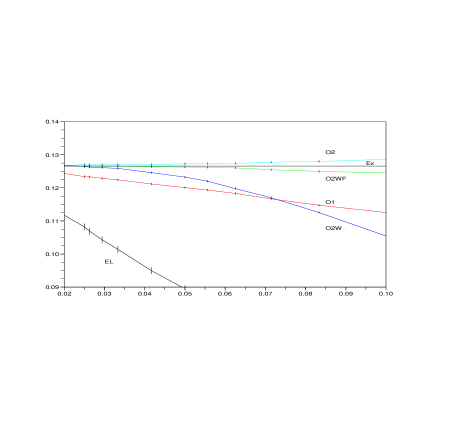
Figure 1: $d=3$, same parameters as for Table 1. In the left (resp. right) side is plotted (50) (resp. $\mathbb{E}\left[\sum_{1\leq i\neq j\leq d}(\hat{X}^{N}_{T})_{i,j}\right]$) in function of the time step $1/N$. The width of each point represents the $95\%$ confidence interval ($10^{7}$ scenarios for the modified Euler scheme and $10^{8}$ for the others).

4 Financial application of correlation processes

In this section, we focus on the modeling of the dependence between $d$ risky assets. We will denote by $S^{1}_{t},\dots,S^{d}_{t}$ their value at time $t$, and we set $\log(S_{t})=(\log(S^{1}_{t}),\dots,\log(S^{d}_{t}))^{T}$. Basically if we exclude jumps, we can assume that the assets follow under a risk neutral probability space $(\Omega,\mathcal{F},\mathbb{P})$ the following dynamics:

$$d\log(S^{i}_{t})=\left(r-\frac{1}{2}(\Sigma_{t})_{i,i}\right)dt+(\sqrt{\Sigma_{t}}dB_{t})_{i},\ 1\leq i\leq d$$ (51)

where $r$ is the interest rate, $(B_{t},t\geq 0)$ is a $d$-dimensional standard Brownian motion and $(\Sigma_{t},t\geq 0)$ is an adapted ${\mathcal{S}_{d}^{+}(\mathbb{R})}$-valued process. This process describes the instantaneous covariance of the stocks

$$\langle d\log(S^{i}_{t}),d\log(S^{j}_{t})\rangle=(\Sigma_{t})_{i,j}dt,$$ (52)

and $\sqrt{(\Sigma_{t})_{i,i}}$ is usually called the volatility of the asset $S^{i}_{t}$.

Modelling directly the whole covariance process $(\Sigma_{t},t\geq 0)$ is not an easy task. This path has recently been explored by Gourieroux and Sufana [15]. Their model has been enhanced by Da Fonseca et al. [9]. They assume that $(\Sigma_{t},t\geq 0)$ is a Wishart process and consider a dynamics that is a natural extension of the famous Heston model [16] to $d$ stocks. Since Wishart processes are closely connected to MRC processes, we will discuss in detail their model in Section 4.1. In particular, we explain why, in our opinion, it can be hardly used in practice when the number of assets is large (say $d\geq 5$).

Instead, the common practice of the market is to start with modeling the volatility $\sigma^{i}_{t}$ of each stock $S^{i}_{t}$. Then, the dependence is modeled by a correlation process $(C_{t},t\geq 0)$, so that the covariance process is defined by

$$\Sigma_{t}=diag(\sigma^{1}_{t},\dots,\sigma^{d}_{t})C_{t}diag(\sigma^{1}_{t},\dots,\sigma^{d}_{t}).$$

Thus, if we consider the following dynamics for the assets

$$d\log(S^{i}_{t})=\left(r-\frac{1}{2}(\sigma^{i}_{t})^{2}\right)dt+\sigma^{i}_{t}(\sqrt{C_{t}}dB_{t})_{i},\ 1\leq i\leq d,$$ (53)

we get back the same instantaneous covariance given as (52). This bottom-up approach has many advantages. Indeed, the modelling of individual stocks is well documented and handled every day by the financial desks. Besides, the choice of the volatility model is free and can be chosen at one’s convenience. For example, we can take a local volatility model ($\sigma^{i}_{t}=\sigma(t,S^{i}_{t})$) or a stochastic volatility model such as Heston model, or a local stochastic volatility model [3]. The calibration of the single stocks can be thus performed separately, before the calibration of the correlation process. There is still few literature that brings on fitting the correlation to market data. Today, the only liquid and quoted derivatives that bring on the dependence between assets are index options. Recently, Langnau [22] and Reghai [25] focused on the calibration of some particular local correlation models (i.e. $C_{t}=C(t,S^{1}_{t},\dots,S^{d}_{t})$) to index option prices. Under a slightly different setting, Jourdain and Sbai [18] have also considered this issue. However, there is still up to our knowledge very few studies on stochastic correlation modelling. We will discuss in Section 4.2 how MRC processes and possible extensions could be used for that purpose.

4.1 The Wishart stochastic covariance model

Da Fonseca et al. [9] assume that $(\Sigma_{t},t\geq 0)$ follows a Wishart process

$$d\Sigma_{t}=\left({\alpha}aa^{T}+b\Sigma_{t}+\Sigma_{t}b^{T}\right)dt+\sqrt{\Sigma_{t}}dW_{t}a+a^{T}dW_{t}^{T}\sqrt{\Sigma_{t}}$$ (54)

with $\alpha\geq d-1$, $a,b\in{\mathcal{M}_{d}(\mathbb{R})}$. The vector Brownian motion $B$ and the matrix Brownian motion $W$ may be correlated as follows:

$$dB_{t}=dW_{t}\rho+\sqrt{1-\|\rho\|_{2}^{2}}d\tilde{B}_{t},\rho\in\mathbb{R}^{d}\ s.t.\ \|\rho\|_{2}\leq 1,$$

where $(\tilde{B}_{t},t\geq 0)$ is a $d$-dimensional Brownian motion independent from $W$. With this choice, the couple $(\log(S_{t}),\Sigma_{t})$ is an affine process, and its characteristic function can be obtained by solving Riccati equations (see Da Fonseca et al. [9]).

From (54), we get that there are Brownian motions $\beta^{i}_{t}$, $i=1,\dots,d$ such that the volatility square of $S^{i}_{t}$ follows:

$$d(\Sigma_{t})_{i,i}=(\alpha(aa^{T})_{i,i}+2\sum_{j=1}^{d}b_{i,j}(\Sigma_{t})_{i,j}dt+2\sqrt{(aa^{T})_{i,i}}\sqrt{(\Sigma_{t})_{i,i}}d\beta^{i}_{t}.$$

The non diagonal elements $(\Sigma_{t})_{i,j}$ for $i\not=j$ can be seen as factors that drive the volatility of each stock. In its full form, the dynamics of one stock and its volatility is not autonomous. This means in practice that it is not possible to calibrate this model separately to single stock market (mainly, European options on single stocks). This calibration has to be done at the same time for all the stocks, which is a priori a very challenging task: many parameters and a lot of data are involved when the number of assets $d$ gets large.

Then, one may want to recover autonomous dynamics for each stock in order to calibrate them separately. Within this model, the only possible choice is to assume that $b$ is a diagonal matrix. In this case, $(\Sigma_{t})_{i,i}$ follows a CIR diffusion and the couple $((\Sigma_{t})_{i,i},S^{i}_{t})$ follows an Heston model [16]: there are independent Brownian motions $\beta^{i},\ \gamma^{i}$ such that

$$d\log(S_{t}^{i}) = (r-\frac{(\Sigma_{t})_{i,i}}{2})dt+\sqrt{(\Sigma_{t})_{i,i}}\left(\tilde{\rho}^{i}d\beta^{i}_{t}+\sqrt{1-(\tilde{\rho}^{i})^{2}}d\gamma^{i}_{t}\right)$$

$$d(\Sigma_{t})_{i,i} = \left(\alpha(a^{T}a)_{i,i}+2b_{i,i}(\Sigma_{t})_{i,i}\right)dt+2\sqrt{(a^{T}a)_{i,i}}\sqrt{(\Sigma_{t})_{i,i}}d\beta_{t}^{i},$$

$$\tilde{\rho}^{i} = \frac{(a^{T}\rho)^{i}}{\sqrt{(a^{T}a)_{i,i}}}=\frac{\sum_{k=1}^{d}a_{k,i}\rho^{i}}{\sqrt{\sum_{k=1}^{d}a_{k,i}^{2}}}.$$

In practice, each individual stock could be then calibrated like in the Heston model. Unfortunately, there are further restrictions implied by this model and especially that $\alpha\geq d-1$, which is the condition that ensures the existence of the Wishart process. This is unlikely because when calibrating Heston to market data, it is typical to get values of $\alpha$ around or below $1$. When modelling many stocks together (say $d\geq 5$), it is then not possible to fit conveniently market data because of this restriction on $\alpha$.

Last, one of the main feature of the model (54) is the Affine property. It allows to obtain the characteristic function of the stocks by solving Riccati differential equations. Then, the pricing of European style options can be made by using Fourier inversion. This approach is known to be very efficient in a one-dimensional framework (see Carr and Madan [6]) and has been used successfully by Da Fonseca et al.[9] to price Best-of options with $d=2$ assets. However, when the number of assets $d$ is much larger, the Fourier inversion requires an integration in dimension $d$ and can no longer be computed quickly. Unless the payoff has a very particular structure to reduce the dimension, the pricing by Fourier inversion is no longer competitive with respect to Monte-Carlo methods and the Affine property does not really give a crucial advantage in terms of computational methods.

For all these reasons, we believe that this model can be used successfully in practice for a small number of stocks ($d=2,3$) but is instead inadequate to model a large basket.

4.2 Towards a stochastic correlation model

Now, we would like to discuss the application of the MRC processes under the framework (53). The first natural idea would be simply to take $(C_{t})_{t\geq 0}\sim MRC_{d}(C_{0},\kappa,c,a)$. With this choice, we would get analytical formulas for correlation swaps. Indeed, a correlation swap between assets $S^{i}_{t}$ and $S^{j}_{t}$ ($i\not=j$) with maturity $T$ has, up to a discount factor, the following price:

$$\mathbb{E}\left[\frac{1}{T}\int_{0}^{T}(C_{t})_{i,j}dt\right]=\frac{1}{(\kappa_{i}+\kappa_{j})T}\left[(C_{0})_{i,j}(1-e^{-(\kappa_{i}+\kappa_{j})T})-c_{i,j}(1-e^{-(\kappa_{i}+\kappa_{j})T}-(\kappa_{i}+\kappa_{j})T)\right].$$ (55)

To be precise, the payoff of a correlation swap is defined as the average over the period $[0,T]$ of the daily correlation of log-returns $\frac{\log\left(\frac{S^{i}_{t+\Delta}}{S^{i}_{t}}\right)\log\left(\frac{S^{j}_{t+\Delta}}{S^{j}_{t}}\right)}{{\sqrt{\log\left(\frac{S^{i}_{t+\Delta}}{S^{i}_{t}}\right)^{2}}\sqrt{\log\left(\frac{S^{j}_{t+\Delta}}{S^{j}_{t}}\right)^{2}}}}$ and is here approximated by $\frac{1}{T}\int_{0}^{T}(C_{t})_{i,j}dt$. Unfortunately, up to now, correlation swaps are not quoted on the markets and are only dealt over the counter. It is then not possible to get data on their prices in order to calibrate $\kappa$, $c$ and $C_{0}$, which would have been very tractable thanks to formula (55).

The only quoted options that bring on the dependence between assets are index options. We have been kindly given by Julien Guyon at Société Générale market data on the DAX index at the 4th October 2010. He provides us with data on European index option prices as well as parametrized local volatility functions $\sigma^{i}(t,x)$ that are already calibrated to options price on each asset. We thus assume in the sequel the dynamics (53) for the stocks with $\sigma^{i}_{t}=\sigma^{i}(t,S^{i}_{t})$. We will also denote

$$I_{t}=\sum_{i=1}^{d}\alpha_{i}S^{i}_{t}$$

the index value and will assume constant weights $\alpha_{i}$ such that $\sum_{i=1}^{d}\alpha_{i}=1$. These weights are given in Table 2 for the DAX.

SIEMENS	BASF	BAYER	E-ON	DAIMLER	ALLIANZ	SAP	D. TELEKOM	D. BANK	RWE
9.91	8.03	7.97	7.67	7.35	6.97	6.01	5.6	5.06	3.86
M-RUECK	LINDE	BMW	VW	D. POST	ADIDAS	D. BOERSE	FRESENIUS-MC	THYSS. KRUPP	MAN
3.23	3.06	2.92	2.26	2.05	1.76	1.65	1.63	1.52	1.47
HENKEL	SDF	LUFTHANSA	METRO	INFINEON	HEIDEL.	FRESENIUS	BEIERSDORF	COMMERZBANK	MERCK
1.29	1.17	1.16	1.12	1.02	0.94	0.9	0.86	0.84	0.74

Table 2: DAX index composition, in percentage (4 October 2010)

To calibrate MRC processes to index options, it is desirable to reduce the number of parameters. We will assume in the sequel with a slight abuse of notation that $\kappa=\kappa I_{d}$, $a=aI_{d}$ with $\kappa,a\in\mathbb{R}_{+}^{*}$, $c_{i,j}=\mathbbm{1}_{i=j}+\rho\mathbbm{1}_{i\not=j}$ for $\rho\in[-1/(d-1),1]$ and $C_{0}=c$. Condition (3) is then simply equivalent to $2\kappa(1-\rho)\geq(d-2)a^{2}$, but we will assume in addition that

$$2\kappa(1-\rho)\geq(d-1)a^{2}$$

in order to take advantage of the $O(d^{3})$ discretization scheme given by (49). Thus, $C_{t}$ follows the following dynamics

$$C_{t}=c+2\kappa\int_{0}^{t}(C_{s}-c)ds+a\sum_{n=1}^{d}\int_{0}^{t}\left(\sqrt{C_{s}-C_{s}e_{d}^{n}C_{s}}dW_{s}e_{d}^{n}+e_{d}^{n}dW_{s}^{T}\sqrt{C_{s}-C_{s}e_{d}^{n}C_{s}}\right),$$ (56)

and we assume that the Brownian motion $W$ is independent from the Brownian motion $B$ that drives the stocks (53). We would like to calibrate such a process to European index option prices. To do so, we first calculate the value $\rho$ such that the constant correlation model $\mathbbm{1}_{i=j}+\rho\mathbbm{1}_{i\not=j}$ fits the at the money implied volatility. Then, we use this value and look at the impact of $\kappa$ and $a$. Figure 2 illustrates these results. As one could expected, this model gives a smile which is not enough sloping and is unable to fit the volatility skew. The parameters $\kappa$ and $a$ have no impact on the slope of the smile.

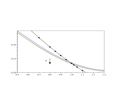
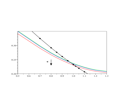
Figure 2: In both graphics, the line with diamonds indicate the market $1$ year implied volatility. We plot the implied given by model (56) with $\rho=0.67968$ and use the parametrization $a=\sqrt{\frac{2\kappa\varepsilon}{d-1}(1-\rho)},$ with $\varepsilon\in[0,1]$. Left: $\kappa=100$ and $\varepsilon\in\left\{0,0.6,1\right\}$. Right: $\varepsilon=0.5$ and $\kappa\in\left\{1,20,100\right\}.$ These curves are obtained with $10^{6}$ Monte-Carlo samples and discretization time step $0.025.$

The reason of this too flat smile is that the correlation is not related to the index price, while the market would expect that the correlation is high (resp. low) when the index is low (resp. high). There are at least two ways to correct this. First, one may assume some dependence between the Brownian motions $W$ and $B$, which would be very analogous to what is made for stochastic volatility models. This requires to find an adequate way to correlate these Brownian motion from a financial point of view that is also tractable for simulation purposes. We have left this for further research.

The second way to make depend the correlation in function of the index value is simply to assume a local correlation model $C(t,I_{t})$ with $C:\mathbb{R}_{+}\times\mathbb{R}_{+}^{*}\rightarrow{\mathfrak{C}_{d}(\mathbb{R})}$ and keep $W$ and $B$ independent. This approach has been considered by Reghai [25]. In Ahdida [1], it is shown that the following parametric form

$$C(t,I_{t})_{i,j}=\mathbbm{1}_{i=j}+\rho(t,I_{t})\mathbbm{1}_{i\not=j},\text{ with }\rho(t,I_{t})=\max\left(\frac{1}{1+\eta\left(I_{t}/I_{0}\right)^{\gamma}},\rho_{\min}\right),$$ (57)

with $\eta,\gamma,\rho_{min}\geq 0$ is very tractable to calibrate the index smile at a given maturity. Indeed, it is shown that $\eta$ tunes the implied volatility at the money, $\gamma$ tunes the skew (i.e. the slope at the money of the implied volatility), and $\rho_{min}$ tunes the right tail of the smile. The left hand side of Figure 3 shows the index smile data and the implied volatility given by this model. Also, an extension of this model with time-dependent parameters can be used to fit the index smile for different maturities.

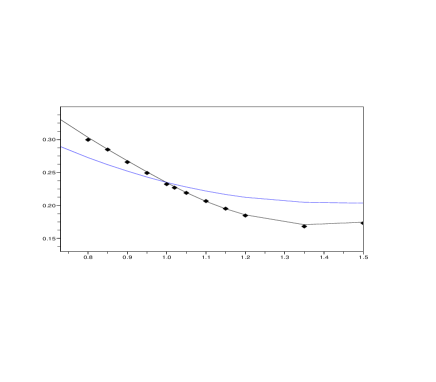
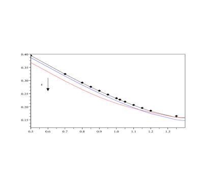
Figure 3: Left: diamonds indicate market $1$ year implied volatility for the DAX. The curve fitting this data is the implied volatility given by the local correlation model (57) with $\gamma=8.672568,$ $\eta=0.500714$ and $\rho_{\min}=0.1.$ The other curve is the implied volatility given by a constant correlation model $(C_{t})_{i,j}=\mathbbm{1}_{i=j}+\rho\mathbbm{1}_{i\not=j}$ that fits the at the money implied volatility: $\rho=0.67968$. Right: With the same values for $\gamma$, $\eta$ and $\rho_{\min}$, we have plotted for $\kappa=100$ and $\varepsilon\in\left\{0,0.3,0.9\right\}$ the implied volatility given by model (58). These curves are obtained with $10^{6}$ Monte-Carlo samples and discretization time step $0.025.$

We want to illustrate now how dynamics such as MRC processes could be used to extend local correlation models and add a new source of randomness. Namely, we consider the following dynamics

$$C_{t}=C_{0}+2\kappa\int_{0}^{t}(C_{s}-C(s,I_{s}))ds+\int_{0}^{t}a(s,I_{s})\sum_{n=1}^{d}\left(\sqrt{C_{s}-C_{s}e_{d}^{n}C_{s}}dW_{s}e_{d}^{n}+e_{d}^{n}dW_{s}^{T}\sqrt{C_{s}-C_{s}e_{d}^{n}C_{s}}\right),$$ (58)

where $\kappa>0$, $a:\mathbb{R}_{+}\times\mathbb{R}_{+}^{*}\rightarrow\mathbb{R}_{+}$ and $C(t,I)$ is defined by (57). The limit case $a(t,x)\equiv 0$, $\kappa=+\infty$ corresponds to the local correlation model. Following the same lines as in the proof of Theorem 12, we could show under some rather mild assumptions on $\rho(t,x)$ and $\sigma^{i}(t,x)$ that the whole SDE on $(C_{t},S^{1}_{t},\dots,S^{d}_{t})$ has a weak solution if $2\kappa(1-\rho(t,x))\geq(d-2)a^{2}(t,x)$ for all $t\geq 0,x>0$, and a unique strong solution if $2\kappa(1-\rho(t,x))\geq da^{2}(t,x)$. To simulate such an SDE, we will simply use the Euler-Maruyama scheme for the stocks and use our scheme for the MRC process with coefficients $\kappa$, $C(t_{i}^{N},I_{t_{i}^{N}})$ and $a(t_{i}^{N},I_{t_{i}^{N}})$ on the time-step $[t^{N}_{i},t^{N}_{i+1}]$. More precisely, we will assume moreover that $2\kappa(1-\rho(t,x))\geq(d-1)a^{2}(t,x)$ and even set

$$a(t,x)=\sqrt{\frac{2\kappa\varepsilon}{d-1}(1-\rho(t,x))},$$

where $\varepsilon\in[0,1]$ is a free parameter. This choice allows to use the $O(d^{3})$ discretization scheme (49) for the MRC process. Starting from the calibrated local correlation model, we have plotted in the right-hand side of Figure 3 the effect of the volatility on the index smile. We have chosen a large value for $\kappa$ so that the model (58) fits the data for $\varepsilon=0$. We see that the volatility of the correlation tends to reduce prices of call option on the index. The same monotonicity was already observed in Figure 2. This indicates some concavity of the index option prices with respect to the correlation.

Last, a natural question is to wonder if this is really necessary to sample a whole correlation process. For example, we could consider the following one-dimensional model

$$C_{t}=\mathbbm{1}_{i=j}+\rho_{t}\mathbbm{1}_{i\not=j},\text{ with }\rho_{t}=\rho_{0}+\kappa\int_{0}^{t}(\rho_{s}-\rho(s,I_{s}))ds+a\int_{0}^{t}\sqrt{\rho_{s}(1-\rho_{s})}dW_{s},$$ (59)

with $\rho_{0}\in[0,1]$, $\kappa>0$, $a\geq 0$. This dynamics would have rather close qualitative features to (58) and is much less demanding in terms of computational effort. To be fair, as far as index modeling is concerned it may be sufficient to parametrize the correlation matrix by a single parameter $\rho_{t}$. The heuristic reason is that index options do not really depend on the individual pairwise correlations $(C_{t})_{i,j}$ but rather depend on an average correlation in the basket. Instead, if the aim is then to price and hedge exotic products on the dependence, it may be relevant to model all the pairwise correlations. To give a caricatural example, an option on the difference of two correlation swaps that pays $(\frac{1}{T}\int_{0}^{T}(C_{t})_{i,j}dt-\frac{1}{T}\int_{0}^{T}(C_{t})_{k,l}dt)^{+}$ is almost surely equal to zero in model (59) or (57), which may basically give an arbitrage. It has instead a non trivial price if $(C_{t})_{t\geq 0}\sim MRC_{d}(C_{0},\kappa,c,a)$ or in model (58).

We have tested MRC type dynamics on index options because they are the only liquid quoted options that bring on dependence. The tractability offered by these processes is not really exploited for such options. Unfortunately today, there is no quoted options that could give the market view on pairwise correlations. However, if an investor has some personal views on correlations between some companies or some industry sectors, processes such as MRC can be a relevant tool to take into account these views and price exotic products. Generally speaking, modelling precisely the dependence between the stocks in order to get a model that prices consistently single-name and basket products is an important challenge in finance, and we hope that processes such as MRC may be tool to achieve it.

Appendix A Some results on correlation matrices

A.1 Linear ODEs on correlation matrices

Let $b\in{\mathcal{S}_{d}(\mathbb{R})}$ and $\kappa\in{\mathcal{M}_{d}(\mathbb{R})}$. In this section, we consider the following linear ODE

$$x^{\prime}(t)=b-(\kappa x(t)+x(t)\kappa^{T}),\ x(0)=x\in{\mathfrak{C}_{d}(\mathbb{R})},$$ (60)

and we are interested in necessary and sufficient conditions on $\kappa$ and $b$ such that

$$\forall x\in{\mathfrak{C}_{d}(\mathbb{R})},\forall t\geq 0,x(t)\in{\mathfrak{C}_{d}(\mathbb{R})}.$$ (61)

Let us first look at necessary conditions. We have for $1\leq i,j\leq d$:

$$x^{\prime}_{i,j}(t)=b_{i,j}-\sum_{k=1}^{d}\kappa_{i,k}x_{k,j}(t)+x_{i,k}(t)\kappa_{j,k}.$$

In particular, we necessarily have $x^{\prime}_{i,i}(t)=0$. This gives for $t=0$, $l\not=i$ and $x(0)=I_{d}+\rho(e^{i,l}_{d}+e^{l,i}_{d})$ that $b_{i,i}-2\kappa_{i,i}-2\rho\kappa_{i,l}=0$ for any $\rho\in[-1,1]$. It comes out that:

$$\kappa_{i,l}=0\text{ if }l\not=i,\ b_{i,i}=2\kappa_{i,i}.$$

Thus, the matrix $\kappa$ is diagonal and we denote $\kappa_{i}=\kappa_{i,i}$. We get $x^{\prime}_{i,j}(t)=b_{i,j}-(\kappa_{i}+\kappa_{j})x_{i,j}(t)$ for $i\not=j$. If $\kappa_{i}+\kappa_{j}=0$, we have $x_{i,j}(t)=x_{i,j}+b_{i,j}t$, which implies that $b_{i,j}=0$. Otherwise, $\kappa_{i}+\kappa_{j}\not=0$ and we get:

$$x_{i,j}(t)=x_{i,j}\exp\left(-(\kappa_{i}+\kappa_{j})t\right)+\frac{b_{i,j}}{\kappa_{i}+\kappa_{j}}\left[1-\exp\left(-(\kappa_{i}+\kappa_{j})t\right)\right].$$

Once again, this implies that $\kappa_{i}+\kappa_{j}>0$ since the initial value $x\in{\mathfrak{C}_{d}(\mathbb{R})}$ is arbitrary. We set for $1\leq i,j\leq d$,

$$c_{i,i}=1,\text{ and for }i\not=j,\ c_{i,j}=\begin{cases}\frac{b_{i,j}}{\kappa_{i}+\kappa_{j}}\text{ if }\kappa_{i}+\kappa_{j}>0\\ 0\text{ if }\kappa_{i}+\kappa_{j}=0.\end{cases}$$ (62)

We have $b=\kappa c+c\kappa$ and for $x=I_{d}$, $c=\lim_{t\rightarrow+\infty}x(t)\in{\mathfrak{C}_{d}(\mathbb{R})}$, and deduce the following result.

Proposition 19

— Let $b\in{\mathcal{S}_{d}(\mathbb{R})}$ and $\kappa\in{\mathcal{M}_{d}(\mathbb{R})}$. If the linear ODE (60) satisfies (61), then we have necessarily:

$$\exists c\in{\mathfrak{C}_{d}(\mathbb{R})},\exists\kappa_{1},\dots,\kappa_{d}\in\mathbb{R},\forall i\not=j,\kappa_{i}+\kappa_{j}\geq 0,\kappa=diag(\kappa_{1},\dots,\kappa_{d})\text{ and }b=\kappa c+c\kappa.$$ (63)

Conversely, let us assume that (63) holds and $b\in{\mathcal{S}_{d}^{+}(\mathbb{R})}$. We get that $\kappa_{i}=b_{i,i}/2\geq 0$ and for $t\geq 0$, $\exp(\kappa t)x(t)\exp(\kappa t)=x+\int_{0}^{t}\exp(\kappa s)b\exp(\kappa s)ds$ is clearly positive semidefinite. Therefore, (61) holds. We get the following result.

Proposition 20

— Let $\kappa_{1},\dots,\kappa_{d}\geq 0$, $\kappa=diag(\kappa_{1},\dots,\kappa_{d})$ and $c\in{\mathfrak{C}_{d}(\mathbb{R})}$. If $\kappa c+c\kappa\in{\mathcal{S}_{d}^{+}(\mathbb{R})}$ or $d=2$, the ODE

$$x^{\prime}(t)=\kappa(c-x)+(c-x)\kappa,\ x(0)=x\in{\mathfrak{C}_{d}(\mathbb{R})}$$ (64)

satisfies (61).

Let us note here that the parametrization of the ODE (64) is redundant when $d=2$, and we can assume without loss of generality that $\kappa_{1}=\kappa_{2}$ for which $\kappa c+c\kappa\in{\mathcal{S}_{d}^{+}(\mathbb{R})}$ is clearly satisfied.

Remark 21

— The condition given by Proposition 19 is necessary but not sufficient, and the condition given by Proposition 20 is sufficient but not necessary. Let $d=3$ and $c=I_{3}$. We can check that for $\kappa=(1,\frac{1}{2},-\frac{1}{2})$, (63) holds but (61) is not true. Also, we can check that for $\kappa=(1,1,-\frac{1}{2})$, (61) holds.

Lemma 22

— Let $\kappa^{1},\kappa^{2}$ be diagonal matrices and $c^{1},c^{2}\in{\mathfrak{C}_{d}(\mathbb{R})}$ such that $\kappa^{1}c^{1}+c^{1}\kappa^{1}+\kappa^{2}c^{2}+c^{2}\kappa^{2}\in{\mathcal{S}_{d}^{+}(\mathbb{R})}$. Then, the ODE

$$x^{\prime}=\kappa^{1}(c^{1}-x)+(c^{1}-x)\kappa^{1}+\kappa^{2}(c^{2}-x)+(c^{2}-x)\kappa^{2}$$

satisfies (61). Besides, $x^{\prime}=\kappa(c-x)+(c-x)\kappa$ with $\kappa=\kappa^{1}+\kappa^{2}\in{\mathcal{S}_{d}^{+}(\mathbb{R})}$ and $c\in{\mathfrak{C}_{d}(\mathbb{R})}$ defined by:

$$c_{i,i}=1,\text{ and for }i\not=j,\ c_{i,j}=\begin{cases}\frac{(\kappa^{1}_{i}+\kappa^{1}_{j})c^{1}_{i,j}+(\kappa^{2}_{i}+\kappa^{2}_{j})c^{2}_{i,j}}{\kappa_{i}+\kappa_{j}}\text{ if }\kappa_{i}+\kappa_{j}>0\\ 0\text{ if }\kappa_{i}+\kappa_{j}=0.\end{cases}$$

Proof.

Since $b=\kappa^{1}c^{1}+c^{1}\kappa^{1}+\kappa^{2}c^{2}+c^{2}\kappa^{2}\in{\mathcal{S}_{d}^{+}(\mathbb{R})}$, (61) holds for $x^{\prime}=b-\kappa x+x\kappa$. Then, we know by (62) that $c$ is a correlation matrix. ∎

A.2 Some algebraic results on correlation matrices

Lemma 23

— Let $c\in{\mathfrak{C}_{d}(\mathbb{R})}$ and $1\leq i\leq d$. Then we have: $c-ce_{d}^{i}c\in{\mathcal{S}_{d}^{+}(\mathbb{R})}$, $(c-ce_{d}^{i}c)_{i,j}=0$ for $1\leq j\leq d$, ${\left({c-ce_{d}^{i}c}\right)}^{[i]}={{c}^{[i]}-c^{i}(c^{i})^{T}}$ and:

$${\left(\sqrt{c-ce_{d}^{i}c}\right)}^{[i]}=\sqrt{{c}^{[i]}-c^{i}(c^{i})^{T}}\text{ and }\left(\sqrt{c-ce_{d}^{i}c}\right)_{i,j}=0.$$

Besides, if $c\in{\mathfrak{C}_{d}^{*}(\mathbb{R})}$, ${c}^{[i]}-c^{i}(c^{i})^{T}\in\mathcal{S}_{d-1}^{+,*}(\mathbb{R})$.

Proof.

Up to a permutation, it is sufficient to prove the result for $i=1$. We have

$$c-ce_{d}^{1}c=\left(\begin{array}[]{cc}0&0_{d-1}^{T}\\ 0_{d-1}&{c}^{[1]}-c^{1}(c^{1})^{T}\end{array}\right)=aca^{T},\text{ with }a=\left(\begin{array}[]{cc}0&0_{d-1}\\ -c^{1}&I_{d-1}\end{array}\right)\in{\mathcal{S}_{d}^{+}(\mathbb{R})}.$$

Besides, we have $\textup{Rk}(aca^{T})=\textup{Rk}(a\sqrt{c})=d-1$ when $c\in{\mathfrak{C}_{d}^{*}(\mathbb{R})}$, which gives ${c}^{[i]}-c^{i}(c^{i})^{T}\in\mathcal{S}_{d-1}^{+,*}(\mathbb{R})$. ∎

Lemma 24

— Let $c\in{\mathfrak{C}_{d}(\mathbb{R})}$ and $1\leq n\leq d$. Then $I_{d}-\sqrt{c}e_{d}^{n}\sqrt{c}\in{\mathcal{S}_{d}^{+}(\mathbb{R})}$ and is such that

$$\sqrt{I_{d}-\sqrt{c}e_{d}^{n}\sqrt{c}}=I_{d}-\sqrt{c}e_{d}^{n}\sqrt{c}.$$

Proof.

The matrix $(\sqrt{c}e_{d}^{n}\sqrt{c})_{i,j}=(\sqrt{c})_{i,n}(\sqrt{c})_{j,n}$ is of rank $1$ and $\sum_{j=1}^{d}(\sqrt{c}e_{d}^{n}\sqrt{c})_{i,j}(\sqrt{c})_{j,n}=(\sqrt{c})_{i,n}$ since $\sum_{j=1}^{d}(\sqrt{c})_{j,n}^{2}=c_{j,j}=1$. Therefore $((\sqrt{c})_{i,n})_{1\leq i\leq d}$ is an eigenvector, and the eigenvalues of $I_{d}-\sqrt{c}e_{d}^{n}\sqrt{c}$ are $0$ and $1$ (with multiplicity $d-1$). ∎

Lemma 25

— Let $q\in\mathcal{S}^{+}_{d}(\mathbb{R})$ be a matrix with rank $r$. Then there is a permutation matrix $p$, an invertible lower triangular matrix $m_{r}\in\mathcal{G}_{r}(\mathbb{R})$ and $k_{r}\in\mathcal{M}_{d-r\times r}(\mathbb{R})$ such that:

$$pqp^{T}=mm^{T},\,\,m=\left(\begin{array}[]{cc}m_{r}&0\\ k_{r}&0\\ \end{array}\right).$$

The triplet $(m_{r},k_{r},p)$ is called an extended Cholesky decomposition of $q$.

The proof of this result and a numerical procedure to get such a decomposition can be found in Golub and Van Loan ([13], Algorithm 4.2.4). When $r=d$, we can take $p=I_{d}$, and $m_{r}$ is the usual Cholesky decomposition.

Lemma 26

— Let $c\in{\mathfrak{C}_{d}(\mathbb{R})}$, $r=\textup{Rk}((c_{i,j})_{2\leq i,j\leq d})$ and $(m_{r},k_{r},\tilde{p})$ an extended Cholesky decomposition of $(c_{i,j})_{2\leq i,j\leq d}$. We set $p=\left(\begin{array}[]{c c}1&0\\ 0&\tilde{p}^{T}\\ \end{array}\right)$, $m=\left(\begin{array}[]{c|c c}1&0&0\\ \hline\cr 0&m_{r}&0\\ 0&k_{r}&0\\ \end{array}\right)$ and $\check{c}=\left(\begin{array}[]{c|c c}1&(m^{-1}_{r}c_{1}^{r})^{T}&0\\ \hline\cr m^{-1}_{r}c_{1}^{r}&I_{r}&0\\ 0&0&I_{d-r-1}\\ \end{array}\right)$, where $c^{r}_{1}\in\mathbb{R}^{r}$, with $(c^{r}_{1})_{i}=(p^{T}cp)_{1,i+1}$ for $1\leq i\leq r$. We have:

$$c=pm\check{c}m^{T}p^{T}\text{ and }\check{c}\in{\mathfrak{C}_{d}(\mathbb{R})}.$$

Proof.

By straightforward block-matrix calculations, on has to check that the vector $c_{1}^{r,d}\in\mathbb{R}^{d-(r+1)}$ defined by $(c_{1}^{r,d})_{i}=(p^{T}cp)_{1,i}$ for $r+1\leq i\leq d$ is equal to $k_{r}m_{r}^{-1}c_{1}^{r}$. To get this, we introduce the matrix $q=\left(\begin{array}[]{c|cc}1&0&0\\ \hline\cr 0&m_{r}&0\\ 0&k_{r}&I_{d-r-1}\\ \end{array}\right)$ and have $q^{-1}=\left(\begin{array}[]{c|cc}1&0&0\\ \hline\cr 0&m^{-1}_{r}&0\\ 0&-k_{r}m^{-1}_{r}&I_{d-r-1}\\ \end{array}\right)$. Since the matrix

$$q^{-1}p^{T}cp(q^{-1})^{T}=\left(\begin{array}[]{c|c c}1&(m^{-1}_{r}c_{1}^{r})^{T}&(c_{1}^{r,d}-k_{r}m_{r}^{-1}c_{1}^{r})^{T}\\ \hline\cr m^{-1}_{r}c_{1}^{r}&I_{r}&0\\ c_{1}^{r,d}-k_{r}m_{r}^{-1}c_{1}^{r}&0&0\\ \end{array}\right)$$

is positive semidefinite, we have $c_{1}^{r,d}=k_{r}m_{r}^{-1}c_{1}^{r}$, $\left(\begin{array}[]{c c}1&(m^{-1}_{r}c_{1}^{r})^{T}\\ m^{-1}_{r}c_{1}^{r}&I_{r}\end{array}\right)\in\mathcal{S}_{r+1}^{+}(\mathbb{R})$ and thus $\check{c}\in{\mathfrak{C}_{d}(\mathbb{R})}$. ∎

Appendix B Some auxiliary results

B.1 Calculation of quadratic variations

Lemma 27

— Let $(\mathcal{F}_{t})_{t\geq 0}$ denote the filtration generated by $(W_{t},t\geq 0)$. We consider a process $(Y_{t})_{t\geq 0}$ valued in ${\mathcal{S}_{d}(\mathbb{R})}$ such that

$$dY_{t}=B_{t}dt+\sum_{n=1}^{d}(A_{t}^{n}dW_{t}e_{d}^{n}+e_{d}^{n}dW_{t}^{T}(A_{t}^{n})^{T}),$$

where $(A^{n}_{t})_{t\geq 0}$, $(B_{t})_{t\geq 0}$ are continuous $(\mathcal{F}_{t})$-adapted processes respectively valued in ${\mathcal{M}_{d}(\mathbb{R})}$, and ${\mathcal{S}_{d}(\mathbb{R})}$. Then, we have for $1\leq i,j,k,l\leq d$:

$$d\langle Y_{i,j},Y_{k,l}\rangle_{t}=\left[\mathbbm{1}_{i=k}(A^{i}_{t}(A^{i}_{t})^{T})_{j,l}+\mathbbm{1}_{i=l}(A^{i}_{t}(A^{i}_{t})^{T})_{j,k}+\mathbbm{1}_{j=k}(A^{j}_{t}(A^{j}_{t})^{T})_{i,l}+\mathbbm{1}_{j=l}(A^{j}_{t}(A^{j}_{t})^{T})_{i,k}\right]dt$$ (65)

Proof.

Since $(A^{n}_{t}dW_{t}e^{n}_{d})_{i,j}=\mathbbm{1}_{j=n}(A^{j}_{t}dW_{t})_{i,j}$ and $(e^{n}_{d}dW_{t}^{T}(A^{n}_{t})^{T})_{i,j}=\mathbbm{1}_{i=n}(A^{i}_{t}dW_{t})_{j,i}$, we get:

$$d(Y_{t})_{i,j}=(B_{t})_{i,j}dt+\sum_{n=1}^{d}(A^{j}_{t})_{i,n}(dW_{t})_{n,j}+(A^{i}_{t})_{j,n}(dW_{t})_{n,i}.$$

Then, $d\langle Y_{i,j},Y_{k,l}\rangle_{t}=\left[\mathbbm{1}_{j=l}\sum_{n=1}^{d}(A^{j}_{t})_{i,n}(A^{j}_{t})_{k,n}+\mathbbm{1}_{j=k}\sum_{n=1}^{d}(A^{j}_{t})_{i,n}(A^{j}_{t})_{l,n}+\mathbbm{1}_{i=l}\sum_{n=1}^{d}(A^{i}_{t})_{j,n}(A^{i}_{t})_{k,n}\right.$
$\left.+\mathbbm{1}_{i=k}\sum_{n=1}^{d}(A^{i}_{t})_{j,n}(A^{i}_{t})_{l,n}\right]dt$, which precisely gives (65). ∎

Lemma 28

— Let us consider $x\in{\mathfrak{C}_{d}^{*}(\mathbb{R})}$, and $(X_{t})_{t\geq 0}$ a solution of the SDE $\eqref{SDE_CORR}$. Let $\tau$ denote the stopping time defined as $\tau=\{t\geq 0,X_{t}\not\in{\mathfrak{C}_{d}^{*}(\mathbb{R})}\}$. Then, there exists a real Brownian motion $(\beta_{t})_{t\geq 0}$ such that for $0\leq t<\tau$,

$$\frac{d(\det(X_{t}))}{\det(X_{t})} = \textup{Tr}[X_{t}^{-1}(\kappa c+c\kappa-(d-2)a^{2})]dt-\textup{Tr}(2\kappa+a^{2})dt+2\sqrt{\textup{Tr}\left[a^{2}(X_{t}^{-1}-I_{d})\right]}d\beta_{t},$$ (66)

$$d\log(\det(X_{t})) = \textup{Tr}[X_{t}^{-1}(\kappa c+c\kappa-da^{2})]dt-\textup{Tr}(2\kappa-a^{2})dt+2\sqrt{\textup{Tr}\left[a^{2}(X_{t}^{-1}-I_{d})\right]}d\beta_{t}.$$ (67)

Proof.

First, let us recall that $\forall i,j,k,l\in\{1,\ldots,d\},\,\,\forall x\in{\mathcal{S}_{d}^{+,*}(\mathbb{R})}\,\,$ $\partial_{i,j}\det(x)=(\textup{adj}(x))_{i,j}=\det(x)x^{-1}_{i,j},$ $\partial_{k,l}\partial_{i,j}(\det(x))=\det(x)(x^{-1}_{l,k}x^{-1}_{i,j}-x^{-1}_{l,j}x^{-1}_{i,k})$. Since $x$ is symmetric, we have in particular that $\partial_{k,l}\partial_{i,j}(\det(x))=0$ if $i=l$ or $j=k$. Itô’s Formula gives for $t<\tau$:

$$\frac{d(\det(X_{t}))}{\det(X_{t})} = \sum_{1\leq i,j\leq d}(X_{t}^{-1})_{i,j}d(X_{t})_{i,j}+\frac{1}{2}\sum_{\begin{subarray}{c}1\leq i,j\leq d\\ 1\leq k,l\leq d\end{subarray}}\left((X_{t}^{-1})_{i,j}(X_{t}^{-1})_{k,l}-(X_{t}^{-1})_{i,k}(X_{t}^{-1})_{j,l}\right)\langle d(X_{t})_{i,j},d(X_{t})_{k,l}\rangle.$$

On the one hand we have

$$\sum_{1\leq i,j\leq d}(X_{t}^{-1})_{i,j}d(X_{t})_{i,j} = \textup{Tr}[X_{t}^{-1}(\kappa c+c\kappa)]dt-\textup{Tr}(2\kappa)dt+2\sum_{i=1}^{d}a_{i}\textup{Tr}\left[X_{t}^{-1}e_{d}^{i}dW_{s}^{T}\sqrt{X_{t}-X_{t}e_{d}^{i}X_{t}}\right].$$

On the other hand we get by (1.1):

$$\sum_{\begin{subarray}{c}1\leq i,j\leq d\\ 1\leq k,l\leq d\end{subarray}}\left((X_{t}^{-1})_{i,j}(X_{t}^{-1})_{k,l}-(X_{t}^{-1})_{i,k}(X_{t}^{-1})_{j,l}\right)\langle d(X_{t})_{i,j},d(X_{t})_{k,l}\rangle$$

$$= \sum_{\begin{subarray}{c}1\leq i,j\leq d\\ 1\leq k,l\leq d\end{subarray}}\left((X_{t}^{-1})_{i,j}(X_{t}^{-1})_{k,l}-(X_{t}^{-1})_{i,k}(X_{t}^{-1})_{j,l}\right)\times\left\{a_{j}^{2}\mathbbm{1}_{j=k}(X_{t}-X_{t}e_{d}^{j}X_{t})_{i,l}\right.$$

$$\,\,\,\,\,\,\,+a_{j}^{2}\mathbbm{1}_{j=l}(X_{t}-X_{t}e_{d}^{j}X_{t})_{i,k}+a_{i}^{2}\mathbbm{1}_{i=l}(X_{t}-X_{t}e_{d}^{i}X_{t})_{j,k}\left.+a_{i}^{2}\mathbbm{1}_{i=k}(X_{t}-X_{t}e_{d}^{i}X_{t})_{j,l}\right\}$$

$$= \sum_{j=1}^{d}\left(\sum_{1\leq i,k\leq d}a_{j}^{2}(X_{t}-X_{t}e_{d}^{j}X_{t})_{i,k}\left((X_{t}^{-1})_{i,j}(X_{t}^{-1})_{k,j}-(X_{t}^{-1})_{i,k}(X_{t}^{-1})_{j,j}\right)\right)$$

$$+\sum_{i=1}^{d}\left(\sum_{1\leq j,l\leq d}a_{i}^{2}(X_{t}-X_{t}e_{d}^{i}X_{t})_{j,l}\left((X_{t}^{-1})_{i,j}(X_{t}^{-1})_{i,l}-(X_{t}^{-1})_{i,i}(X_{t}^{-1})_{j,l}\right)\right)$$

$$= 2\sum_{i=1}^{d}a_{i}^{2}\left(\textup{Tr}\left[(X_{t}-X_{t}e_{d}^{i}X_{t})X_{t}^{-1}e_{d}^{i}X_{t}^{-1}\right]-(X_{t}^{-1})_{i,i}\textup{Tr}\left[(X_{t}-X_{t}e_{d}^{i}X_{t})X_{t}^{-1}\right]\right).$$

Since $X_{t}\in{\mathfrak{C}_{d}^{*}(\mathbb{R})}$, we obtain that $\textup{Tr}\left[(X_{t}-X_{t}e_{d}^{i}X_{t})X_{t}^{-1}e_{d}^{i}X_{t}^{-1}\right]=(X_{t}^{-1})_{i,i}-1$ and $\textup{Tr}\left[X_{t}^{-1}(X_{t}-X_{t}e_{d}^{i}X_{t})\right]=d-(X_{t})_{i,i}=d-1$. We finally get:

$$\frac{d(\det(X_{t}))}{\det(X_{t})}=\textup{Tr}[X_{t}^{-1}(\kappa c+c\kappa-(d-2)a^{2})]dt-\textup{Tr}(2\kappa+a^{2})dt+2\sum_{i=1}^{d}a_{i}\textup{Tr}\left[X_{t}^{-1}e_{d}^{i}dW_{s}^{T}\sqrt{X_{t}-X_{t}e_{d}^{i}X_{t}}\right].$$ (68)

Now, we compute the quadratic variation of $\det(X_{t})$ by using (1.1):

$$\frac{d\langle\det(X)\rangle_{t}}{\det(X_{t})^{2}} = \sum_{\begin{subarray}{c}1\leq i,j\leq d\\ 1\leq k,l\leq d\end{subarray}}(X_{t}^{-1})_{i,j}(X_{t}^{-1})_{k,l}\left\{a_{j}^{2}\mathbbm{1}_{j=k}(X_{t}-X_{t}e_{d}^{j}X_{t})_{i,l}+a_{j}^{2}\mathbbm{1}_{j=l}(X_{t}-X_{t}e_{d}^{j}X_{t})_{i,k}\right.$$

$$\ \left.+a_{i}^{2}\mathbbm{1}_{i=l}(X_{t}-X_{t}e_{d}^{i}X_{t})_{j,k}+a_{i}^{2}\mathbbm{1}_{i=k}(X_{t}-X_{t}e_{d}^{i}X_{t})_{j,l}\right\}dt$$

$$= 4\sum_{i=1}^{d}a_{i}^{2}\textup{Tr}\left[X_{t}^{-1}e_{d}^{i}X_{t}^{-1}(X_{t}-X_{t}e_{d}^{i}X_{t})\right]dt$$

$$= 4\sum_{i=1}^{d}a_{i}^{2}((X_{t}^{-1})_{i,i}-1)dt=4[\textup{Tr}(a^{2}X_{t}^{-1})-\textup{Tr}(a^{2})]dt.$$

It is indeed nonnegative: we can show by diagonalizing and using the convexity of $x\mapsto 1/x$ that $x^{-1}_{i,i}\geq 1/x_{i,i}=1$. Then, there is a Brownian motion $(\beta_{t},t\geq 0)$ such that (66) holds (see Theorem 3.4.2 in [19]). ∎

Proposition 29

— Let $k,\theta,\eta\geq 0$. For a given $x\in[-1.1],$ let us consider a process $(X_{t}^{x})_{t\geq 0},$ starting from $x,$ and defined as the solution of the following SDE

$$dX_{t}^{x}=k(\theta-X_{t}^{x})dt+\eta\sqrt{1-(X_{t}^{x})^{2}}dB_{t},$$ (69)

where $(B_{t})_{t\geq 0}$ is a real Brownian motion. Then there exists a positive constant $K>0,$ such that

$$\forall t\geq 0,\forall x\in[-1,1],\,\,\mathbb{E}\left[(X_{t}^{x}-x)^{4}\right]\leq Kt^{2}$$

Proof.

For a given $x\in[-1,1],$ we set $f^{x}(y)=(y-x)^{4}$. If we denote $L$ the infinitesimal operator of the process $X_{t}^{x},$ then we notice that $f^{x}(x)=Lf^{x}(x)=0$. Besides, $(x,y)\in[-1,1]^{2}\mapsto L^{2}f^{x}(y)$ is continuous and therefore bounded:

$$\exists K>0,\forall x,y\in[-1,1],\,|L^{2}f^{x}(y)|\leq 2K.$$ (70)

Since the process $(X_{t}^{x})_{t\geq 0}$ is defined on $[-1,1],$ we get by applying twice Itô’s formula:

$$\mathbb{E}\left[f^{x}(X_{t}^{x})\right]=\int_{0}^{t}\int_{0}^{s}\mathbb{E}\left[L^{2}f^{x}(X_{u}^{x})\right]duds.$$

From $\eqref{ineq_L_2},$ one can deduce that ${\Big{|}}\int_{0}^{t}\int_{0}^{s}\mathbb{E}\left[L^{2}f^{x}(X_{u}^{x})\right]duds{\Big{|}}\leq Kt^{2},$ and obtain the final result.

∎

B.2 Some basic results on squared Bessel processes

Lemma 30

— Let $\beta\geq 2$ and $Z_{t}=z+\beta t+2\int_{0}^{t}\sqrt{Z_{s}}dB_{s}$ be a squared Bessel process of dimension $\beta$ starting from $z>0$. Then we have

$$\mathbb{P}(\forall t\geq 0,\int_{0}^{t}\frac{ds}{Z_{s}}<\infty)=1 \int_{0}^{+\infty}\frac{ds}{Z_{s}}=+\infty\,\,a.s.$$ and

Proof.

The first claim is obvious, since the square Bessel process does never touch zero under the condition of $\beta\geq 2.$ (see for instance [17], part 6.1.3). By using a comparison theorem ($\forall t\geq 0,Z_{t}\leq Z^{\prime}_{t}$ a.s. if $\beta\leq\beta^{\prime}$), it is sufficient to prove the second claim for $\beta\in\mathbb{N}$. In this case, it is well known that $(W^{1}_{t}+\sqrt{z})^{2}+\sum_{k=2}^{n}(W^{k}_{t})^{2}$ follows a square Bessel process of dimension $n$, where $(W^{k}_{t},t\geq 0)$ are independent Brownian motion. By the law of the iterated logarithm, $\limsup_{t\rightarrow+\infty}\frac{(W^{k}_{t})^{2}}{2t\log(\log(t))}=1$, which gives the desired result since $\int_{1}^{\infty}\frac{dt}{t\log(\log(t))}=+\infty$. ∎

Lemma 31

— Let $\beta\geq 6$. Let $Z_{t}=1+\beta t+2\int_{0}^{t}\sqrt{Z_{s}}dB_{s}$ be a squared Bessel process of dimension $\beta$ starting from $1$ and $\phi(t)=\int_{0}^{t}\frac{1}{Z_{s}}ds$. Then we have

$$\mathbb{E}[\phi(t)]=t+\frac{4-\beta}{2}t^{2}+O(t^{3}),\ \mathbb{E}[\phi(t)^{2}]=t^{2}+O(t^{3}),\ \mathbb{E}[\phi(t)^{3}]=O(t^{3}).$$

Proof.

For a fixed time $t>0$, the density of $Z_{t}$ is given by:

$$z>0,p(t,z)=\sum_{k=0}^{+\infty}\frac{e^{-\frac{1}{2t}}(\frac{1}{2t})^{k}}{k!}\frac{1}{2t\Gamma(k+\frac{\beta}{2})}(\frac{z}{2t})^{k-1+\frac{\beta}{2}}e^{-\frac{z}{2t}}.$$

Let us consider that $\gamma\in\left\{1,2,3\right\},$ then all negative moments can be written as

$$\mathbb{E}\left[\frac{1}{Z_{t}^{\gamma}}\right]=\sum_{k=0}^{+\infty}\ \frac{e^{-\frac{1}{2t}}(\frac{1}{2t})^{k+\gamma}}{k!}\frac{\Gamma(k+\frac{\beta}{2}-\gamma)}{\Gamma(k+\frac{\beta}{2})}=\sum_{k=0}^{+\infty}\ \frac{e^{-\frac{1}{2t}}(\frac{1}{2t})^{k+\gamma}}{k!}\frac{1}{(k+\frac{\beta}{2}-1)\times\dots\times(k+\frac{\beta}{2}-\gamma)}.$$

We have $\frac{1}{(k+\frac{\beta}{2}-1)}=\frac{1}{k+1}-\frac{\beta-4}{2(k+2)(k+1)}+O(\frac{1}{k^{3}})$, which yields to the following expansion:

$$\mathbb{E}\left[\frac{1}{Z_{t}}\right] = \sum_{k=0}^{+\infty}\frac{e^{-\frac{1}{2t}}(\frac{1}{2t})^{k+1}}{(k+1)!}-(\beta-4)t\sum_{k=0}^{+\infty}\frac{e^{-\frac{1}{2t}}(\frac{1}{2t})^{k+2}}{(k+2)!}+O\left(\frac{t^{2}}{2}\sum_{k=0}^{+\infty}\frac{e^{-\frac{1}{2t}}(\frac{1}{2t})^{k+3}}{(k+3)!}\right)$$ (71)

$$= 1-(\beta-4)t+O(t^{2})$$

The first equality is thus obtained. We use the same argument to get:

$$\mathbb{E}\left[\frac{1}{Z_{t}^{2}}\right] = \sum_{k=0}^{+\infty}\frac{e^{-\frac{1}{2t}}(\frac{1}{2t})^{k+2}}{(k+2)!}+O\left(t\sum_{k=0}^{+\infty}\frac{e^{-\frac{1}{2t}}(\frac{1}{2t})^{k+3}}{(k+3)!}\right)=1+O(t)$$

$$\mathbb{E}\left[\frac{1}{Z_{t}^{3}}\right] = O\left(\sum_{k=0}^{+\infty}\frac{e^{-\frac{1}{2t}}(\frac{1}{2t})^{k+3}}{(k+3)!}\right)=O(1).$$ (72)

By Jensen’s inequality, one can deduce that $\mathbb{E}\left[\left(\int_{0}^{t}\frac{ds}{Z_{s}}\right)^{3}\right]\leq t^{2}\mathbb{E}\left[\int_{0}^{t}\frac{ds}{(Z_{s})^{3}}\right].$ Thanks to the moment expansion in $\eqref{equ2},$ we find the third equality. Finally, by Jensen’s equality, we obtain that

$$\mathbb{E}\left[\left(\int_{0}^{t}\left[\frac{1}{Z_{s}}-1\right]ds\right)^{2}\right]\leq t\mathbb{E}\left[\int_{0}^{t}\left(\frac{1}{Z_{s}}-1\right)^{2}ds\right] = t\mathbb{E}\left[\int_{0}^{t}\frac{ds}{(Z_{s})^{2}}\right]-2t\mathbb{E}\left[\int_{0}^{t}\frac{ds}{(Z_{s})}\right]+t^{2}$$

$$= t^{2}-2t^{2}+t^{2}+O(t^{3})=O(t^{3}).$$

It yields that

$$\mathbb{E}\left[\left(\int_{0}^{t}\left[\frac{1}{Z_{s}}\right]ds\right)^{2}\right] = \mathbb{E}\left[\left(\int_{0}^{t}\left[\frac{1}{Z_{s}}-1\right]ds\right)^{2}\right]-t^{2}+2t\int_{0}^{t}\mathbb{E}\left[\frac{1}{Z_{s}}\right]ds=t^{2}+O(t^{3}).$$

∎

Appendix C A direct proof of Theorem 6

Proof.

From (7) we have $2L_{i}=-\alpha L_{i}^{D}+L_{i}^{M}$, with:

$$L^{D}_{i}=\sum_{\begin{subarray}{c}1\leq j\leq d\\ j\not=i\end{subarray}}x_{\{i,j\}}\partial_{\{i,j\}},\ \ L_{i}^{M}=\sum_{\begin{subarray}{c}1\leq j,k\leq d\\ j\not=i,k\not=i\end{subarray}}(x_{\{j,k\}}-x_{\{i,j\}}x_{\{i,k\}})\partial_{\{i,j\}}\partial_{\{i,k\}}.$$

We want to show that $L_{i}L_{j}=L_{j}L_{i}$ for $i\not=j$. Up to a permutation of the coordinates, $L_{i}$ and $L_{j}$ are the same operators as $L_{1}$ and $L_{2}$. It is therefore sufficient to check that $L_{1}L_{2}=L_{2}L_{1}$. Since $L_{1}L_{2}=L_{1}^{M}L_{2}^{M}-\alpha(L_{1}^{D}L_{2}^{M}+L_{1}^{M}L_{2}^{D})+\alpha^{2}L_{1}^{D}L_{2}^{D}$, it is sufficient to check that the three terms remain unchanged when we exchange indices $1$ and $2$. To do so we write:

$$\begin{split}L_{1}^{M}&={\sum_{\begin{subarray}{c}3\leq i,j\leq d\end{subarray}}(x_{\{i,j\}}-x_{\{1,i\}}x_{\{1,j\}})\partial_{\{1,i\}}\partial_{\{1,j\}}+2\sum_{\begin{subarray}{c}3\leq i\leq d\end{subarray}}(x_{\{2,i\}}-x_{\{1,2\}}x_{\{1,i\}})\partial_{\{1,2\}}\partial_{\{1,i\}}+(1-x_{\{1,2\}}^{2})\partial_{\{1,2\}}^{2}}\\ L_{2}^{M}&={\sum_{\begin{subarray}{c}3\leq k,l\leq d\end{subarray}}(x_{\{k,l\}}-x_{\{2,k\}}x_{\{2,l\}})\partial_{\{2,k\}}\partial_{\{2,l\}}+2\sum_{\begin{subarray}{c}3\leq l\leq d\end{subarray}}(x_{\{1,l\}}-x_{\{1,2\}}x_{\{2,l\}})\partial_{\{1,2\}}\partial_{\{2,l\}}+(1-x_{\{1,2\}}^{2})\partial_{\{1,2\}}^{2}}\\ L_{1}^{D}&=x_{\{1,2\}}\partial_{\{1,2\}}+\sum_{\begin{subarray}{c}3\leq i\leq d\end{subarray}}x_{\{1,i\}}\partial_{\{1,i\}},\ \ \ \ L_{2}^{D}=x_{\{1,2\}}\partial_{\{1,2\}}+\sum_{\begin{subarray}{c}3\leq l\leq d\end{subarray}}x_{\{2,l\}}\partial_{\{2,l\}}.\end{split}$$

By a straightforward but tedious calculation, we get :
$\displaystyle L_{1}^{M}L_{2}^{M}=\underset{\overline{1}}{\underbrace{\sum_{\begin{subarray}{c}3\leq i,j,k,l\leq d\end{subarray}}(x_{\{i,j\}}-x_{\{1,i\}}x_{\{1,j\}})(x_{\{k,l\}}-x_{\{2,k\}}x_{\{2,l\}})\partial_{\{1,i\}}\partial_{\{1,j\}}\partial_{\{2,k\}}\partial_{\{2,l\}}}}$
$\displaystyle+\underset{\tilde{2}}{\underbrace{\sum_{\begin{subarray}{c}3\leq i,j\leq d\end{subarray}}(x_{\{i,j\}}-x_{\{1,i\}}x_{\{1,j\}})\left(2\partial_{\{1,2\}}\partial_{\{2,i\}}\partial_{\{1,j\}}+2\partial_{\{1,2\}}\partial_{\{2,j\}}\partial_{\{1,i\}}\right)}}$
$\displaystyle+2\underset{3}{\underbrace{\sum_{\begin{subarray}{c}3\leq i,j,l\leq d\end{subarray}}(x_{\{i,j\}}-x_{\{1,i\}}x_{\{1,j\}})(x_{\{1,l\}}-x_{\{1,2\}}x_{\{1,l\}})\partial_{\{1,2\}}\partial_{\{2,l\}}\partial_{\{1,i\}}\partial_{\{1,j\}}}}$
$\displaystyle+\underset{4}{\underbrace{\sum_{\begin{subarray}{c}3\leq i,j\leq d\end{subarray}}(x_{\{i,j\}}-x_{\{1,i\}}x_{\{1,j\}})(1-x_{\{1,2\}}^{2})\partial_{\{1,i\}}\partial_{\{1,j\}}\partial_{\{1,2\}}^{2}}}$
$\displaystyle+2\underset{3}{\underbrace{\sum_{\begin{subarray}{c}3\leq i,k,l\leq d\end{subarray}}(x_{\{2,i\}}-x_{\{1,2\}}x_{\{1,i\}})(x_{\{k,l\}}-x_{\{2,k\}}x_{\{2,l\}})\partial_{\{2,k\}}\partial_{\{2,l\}}\partial_{\{1,2\}}\partial_{\{1,i\}}}}$
$\displaystyle+4\sum_{\begin{subarray}{c}3\leq i\leq d\end{subarray}}(x_{\{2,i\}}-x_{\{1,2\}}x_{\{1,i\}})\left(\underset{\tilde{5}}{\underbrace{\partial_{\{1,2\}}^{2}\partial_{\{2,i\}}}}-\underset{\tilde{6}}{\underbrace{\sum_{\begin{subarray}{c}3\leq l\leq d\end{subarray}}x_{\{2,l\}}\partial_{\{1,2\}}\partial_{\{2,l\}}\partial_{\{1,i\}}}}+\underset{\overline{7}}{\underbrace{\sum_{\begin{subarray}{c}3\leq l\leq d\end{subarray}}(x_{\{1,l\}}-x_{\{1,2\}}x_{\{2,l\}})\partial_{\{1,2\}}^{2}\partial_{\{2,l\}}\partial_{\{1,i\}}}}\right)$
$\displaystyle+2\sum_{\begin{subarray}{c}3\leq i\leq d\end{subarray}}(x_{\{2,i\}}-x_{\{1,2\}}x_{\{1,i\}})\left(\underset{\tilde{8}}{\underbrace{-2x_{\{1,2\}}\partial_{\{1,2\}}^{2}\partial_{\{1,i\}}}}+\underset{9}{\underbrace{(1-x_{\{1,2\}}^{2})\partial_{\{1,2\}}^{3}\partial_{\{1,i\}}}}\right)$
$\displaystyle+\underset{4}{\underbrace{\sum_{\begin{subarray}{c}3\leq k,l\leq d\end{subarray}}(x_{\{k,l\}}-x_{\{2,k\}}x_{\{2,m\}})(1-x_{\{1,2\}}^{2})\partial_{\{2,k\}}\partial_{\{2,m\}}\partial_{\{1,2\}}^{2}}}$
$\displaystyle+(1-x_{\{1,2\}}^{2})\left(\sum_{\begin{subarray}{c}3\leq l\leq d\end{subarray}}\underset{9}{\underbrace{2(x_{\{1,l\}}-x_{\{1,2\}}x_{\{2,l\}})\partial_{\{1,2\}}^{3}\partial_{\{2,l\}}}}-\underset{\tilde{10}}{\underbrace{4\sum_{\begin{subarray}{c}3\leq l\leq d\end{subarray}}x_{\{2,l\}}\partial_{\{1,2\}}^{2}\partial_{\{2,l\}}}}\right)$
$\displaystyle+\underset{\overline{11}}{\underbrace{(1-x_{\{1,2\}}^{2})\partial_{\{1,2\}}^{2}((1-x_{\{1,2\}}^{2})\partial_{\{1,2\}}^{2})}}$
In this formula, the terms $\bar{n}$ are already symmetric by exchanging $1$ and $2$. The terms $n$ are paired with the corresponding symmetric term. To analyse the terms $\tilde{n}$, we have to do further calculations. On the one hand,

$$\tilde{10}+\tilde{5} = \sum_{\begin{subarray}{c}3\leq l\leq d\end{subarray}}4x_{\{1,2\}}(x_{\{1,2\}}x_{\{2,l\}}-x_{\{1,l\}})\partial_{\{1,2\}}^{2}\partial_{\{2,l\}}$$

$$\tilde{8} = \sum_{\begin{subarray}{c}3\leq l\leq d\end{subarray}}4x_{\{1,2\}}(x_{\{1,2\}}x_{\{1,l\}}-x_{\{2,l\}})\partial_{\{1,2\}}^{2}\partial_{\{1,l\}},$$

are symmetric together. On the other hand we have

$$\tilde{2}+\tilde{6}=\sum_{\begin{subarray}{c}1\leq i,j\leq d\\ i\neq 1,2,j\neq 1,2\end{subarray}}\left\{4x_{\{i,j\}}-4x_{\{1,i\}}x_{\{1,j\}}-4x_{\{2,i\}}x_{\{2,j\}}+4x_{\{1,i\}}x_{\{2,j\}}x_{\{1,2\}}\right\}\partial_{\{1,2\}}\partial_{\{1,i\}}\partial_{\{2,j\}},$$

which is symmetric.

Now we focus on $L_{1}^{D}L_{2}^{M}+L_{1}^{M}L_{2}^{D}$. We number the terms with the same rule as above, and get:

$$\begin{split}&L_{1}^{D}L_{2}^{M}+L_{1}^{M}L_{2}^{D}=\underset{1}{\underbrace{\sum_{\begin{subarray}{c}3\leq k,l\leq d\end{subarray}}(x_{\{k,l\}}-x_{\{2,l\}}x_{\{2,k\}})x_{\{1,2\}}\partial_{\{2,l\}}\partial_{\{2,k\}}\partial_{\{1,2\}}}}\\ &+2\underset{2}{\underbrace{\sum_{\begin{subarray}{c}3\leq l\leq d\end{subarray}}x_{\{1,2\}}(x_{\{1,l\}}-x_{\{1,2\}}x_{\{2,l\}})\partial_{\{1,2\}}^{2}\partial_{\{2,l\}}}}-2\underset{{3}}{\underbrace{\sum_{\begin{subarray}{c}3\leq l\leq d\end{subarray}}x_{\{1,2\}}x_{\{2,l\}}\partial_{\{2,l\}}\partial_{\{1,2\}}}}+\underset{\overline{4}}{\underbrace{x_{\{1,2\}}\partial_{\{1,2\}}\left\{(1-x_{\{1,2\}}^{2})\partial_{\{1,2\}}^{2}\right\}}}\\ &+\underset{5}{\underbrace{\sum_{\begin{subarray}{c}3\leq i,k,l\leq d\end{subarray}}x_{\{1,i\}}(x_{\{l,k\}}-x_{\{2,k\}}x_{\{2,l\}})\partial_{\{2,k\}}\partial_{\{2,l\}}\partial_{\{1,i\}}}}+\underset{6}{\underbrace{2\sum_{\begin{subarray}{c}3\leq i,l\leq d\end{subarray}}x_{\{1,i\}}(x_{\{1,l\}}-x_{\{1,2\}}x_{\{2,l\}})\partial_{\{1,2\}}\partial_{\{2,l\}}\partial_{\{1,i\}}}}\\ &+2\underset{{7}}{\underbrace{\sum_{\begin{subarray}{c}3\leq i\leq d\end{subarray}}x_{\{1,i\}}\partial_{\{1,2\}}\partial_{\{2,i\}}}}+\underset{8}{\underbrace{\sum_{\begin{subarray}{c}3\leq i\leq d\end{subarray}}x_{\{1,i\}}(1-x_{\{1,2\}}^{2})\partial_{\{1,2\}}^{2}\partial_{\{1,i\}}}}+\underset{1}{\underbrace{\sum_{\begin{subarray}{c}3\leq i,j\leq d\end{subarray}}(x_{\{i,j\}}-x_{\{1,i\}}x_{\{1,j\}})x_{\{1,2\}}\partial_{\{1,2\}}\partial_{\{1,i\}}\partial_{\{1,j\}}}}\\ &+\underset{5}{\underbrace{\sum_{\begin{subarray}{c}3\leq i,j,l\leq d\end{subarray}}x_{\{2,l\}}(x_{\{i,j\}}-x_{\{1,i\}}x_{\{1,j\}})\partial_{\{1,i\}}\partial_{\{1,j\}}\partial_{\{2,l\}}}}+2\underset{2}{\underbrace{\sum_{\begin{subarray}{c}3\leq i\leq d\end{subarray}}x_{\{1,2\}}(x_{\{2,i\}}-x_{\{1,2\}}x_{\{1,i\}})\partial_{\{1,2\}}^{2}\partial_{\{1,i\}}}}\\ &+2\sum_{\begin{subarray}{c}3\leq i\leq d\end{subarray}}(\underset{7}{\underbrace{x_{\{2,i\}}}}-\underset{3}{\underbrace{x_{\{1,i\}}x_{\{1,2\}}}})\partial_{\{1,i\}}\partial_{\{1,2\}}+2\underset{6}{\underbrace{\sum_{\begin{subarray}{c}3\leq i,l\leq d\end{subarray}}x_{\{2,l\}}(x_{\{2,i\}}-x_{\{1,2\}}x_{\{1,i\}})\partial_{\{1,i\}}\partial_{\{1,2\}}\partial_{\{2,l\}}}}\\ &+\underset{\overline{9}}{\underbrace{(1-x_{\{1,2\}}^{2})\partial_{\{1,2\}}^{2}\{x_{\{1,2\}}\partial_{\{1,2\}}\}}}+\underset{8}{\underbrace{\sum_{\begin{subarray}{c}3\leq l\leq d\end{subarray}}(1-x_{\{1,2\}}^{2})x_{\{2,l\}}\partial_{\{1,2\}}^{2}\partial_{\{2,l\}}}}.\end{split}$$

Therefore, $L_{1}^{D}L_{2}^{M}+L_{1}^{M}L_{2}^{D}$ is symmetric when we exchange $1$ and $2$. Last, it is easy to check that $L_{1}^{D}L_{2}^{D}=L_{2}^{D}L_{1}^{D}$, which concludes the proof. ∎

Appendix D A direct construction of a second order scheme for MRC processes

In Section 3, we have presented a second order scheme for Mean-Reverting Correlation processes that is obtained from a second order scheme for Wishart processes. In this section, we propose a second order scheme that is constructed directly by a splitting of the generator of Mean-Reverting Correlation processes. As pointed in (42), it is sufficient to construct a potential second order scheme for ${MRC}_{d}({x},\frac{d-2}{2}e_{d}^{1},I_{d},e_{d}^{1};t)$. Thanks to the transformation given by Proposition 9, it is even sufficient to construct such a scheme when $(x)_{2\leq i,j\leq d}=I_{d-1}$.

Consequently, in the rest of this section, we focus on getting a potential second order scheme for ${MRC}_{d}({x},\frac{d-2}{2}e_{d}^{1},I_{d},e_{d}^{1};t),$ where $(x)_{2\leq i,j\leq d}=I_{d-1}$. By (22), the matrix $x$ is a correlation matrix if $\sum_{i=2}^{d}x_{1,i}^{2}\leq 1$. Besides, the only non constant elements are on the first row (or the first column) and the vector $((X_{t})_{1,i})_{2\ldots d}$ is thus defined on the unit ball $\mathbb{D}$:

$$\mathbb{D}=\left\{x\in\mathbb{R}^{d-1},\,\,\sum_{i=1}^{d-1}x_{i}^{2}\leq 1\right\}.$$ (73)

With a slight abuse of notation, the process $((X_{t})_{i})_{1\ldots d-1}$ will denote the vector $((X_{t})_{1,i+1})_{1\ldots d-1}.$ Its quadratic covariance is given by $d\langle(X_{t})_{i},d(X_{t})_{j}\rangle=\left(\mathbbm{1}_{i=j}-(X_{t})_{i}(X_{t})_{j}\right)dt$, and the infinitesimal generator $L^{1}$ of ${{MRC}_{d}({x},\frac{d-2}{2}e_{d}^{1},I_{d},e_{d}^{1})}$ can be rewritten on $\mathbb{D},$ as

$$L^{1}=-\frac{d-2}{2}\sum_{i=1}^{d-1}x_{i}\partial_{i}+\frac{1}{2}\sum_{1\leq i,j\leq d-1}(\mathbbm{1}_{i=j}-x_{i}x_{j})\partial_{i}\partial_{j}.$$ (74)

One can prove that the following stochastic differential equation

$$\forall 1\leq i\leq d-1,\,\,dM_{t}^{i}=-\frac{d-2}{2}M_{t}^{i}+M_{t}^{i}\sqrt{1-\sum_{j=1}^{d-1}(M_{t}^{j})^{2}}dB_{t}^{1}+(1-(M_{t}^{i})^{2})dB_{t}^{i+1}-M_{t}^{i}\sum_{\begin{subarray}{c}1\leq j\leq{d-1}\\ j\neq i\end{subarray}}M_{t}^{j}dB_{t}^{j+1}$$

is associated to the martingale problem of $L^{1}$, where $(B_{t})_{t\geq 0}$ denotes a standard Brownian motion in dimension $d$. By Theorem (12), there is a unique weak solution $(M_{t})_{t\geq 0}$ that is defined on $\mathbb{D}.$

The scope of this section is to derive a potential second order discretization for the operator $L^{1},$ by using an ad-hoc splitting and the results of Proposition 18. We consider the following splitting

$$L^{1}={\mathcal{L}}^{1}+\sum_{m=1}^{d-1}\mathcal{L}^{m+1},$$ (75)

where we have, for $1\leq m\leq d-1$:

$${\mathcal{L}}^{1}\,\, = \frac{1}{2}\left(1-\sum_{i=1}^{d-1}x_{i}^{2}\right)\sum_{\begin{subarray}{c}1\leq l,k\leq d-1\end{subarray}}x_{k}x_{l}\partial_{k}\partial_{l},$$

$$\mathcal{L}^{m+1} = \frac{1}{2}\left(-\sum_{1\leq k\neq m\leq{d-1}}x_{k}\partial_{k}+(1-x_{m}^{2})^{2}\partial_{m}^{2}-2x_{m}(1-x_{m}^{2})\sum_{1\leq k\neq m\leq{d-1}}x_{k}\partial_{k}\partial_{m}+\sum_{{\small\begin{subarray}{c}1\leq k\neq m\leq{d-1}\\ 1\leq l\neq m\leq{d-1}\end{subarray}}}x_{k}x_{l}x_{m}^{2}\partial_{k}\partial_{l}\right).$$

Thanks to Proposition 18, it is sufficient to focus on getting potential second-order schemes for the operators $\mathcal{L}^{1},\dots,\mathcal{L}^{d}$.

D.1 Potential second order schemes for $\mathcal{L}^{2},\ldots,\mathcal{L}^{d}$

All the generators $\mathcal{L}^{l+1}$, $l=1,\dots,d-1$ have the same solution as $\mathcal{L}^{2}$ up to the permutation of the first coordinate and the $l$-th one. It is then sufficient to focus on the first operator $\mathcal{L}^{2}.$ By straightforward calculus, we find that the following SDE

$$d(X_{t})_{1}=(1-(X_{t})_{1}^{2})dB_{t} \,\,\forall 2\leq i\leq{d-1}\,\,d(X_{t})_{i}=-(X_{t})_{i}\left(\frac{dt}{2}+(X_{t})_{1}dB_{t}\right),\ X_{0}=x\in\mathbb{D},$$ , (76)

is well a solution of the martingale problem for the generator $\mathcal{L}^{2}$. The SDE that defines $(X_{t})_{1}$ is autonomous. Since $x_{1}\in[-1,1]$, it has clearly a unique strong valued in $[-1,1]$. It yields that the SDE $\eqref{SDE_opL2}$ has a unique strong solution on $\mathbb{R}^{d}.$ To prove that $(X_{t})_{t\geq 0}$ takes values in $\mathbb{D}$ we consider $V_{t}=\sum_{i=1}^{d}(X_{t})_{i}^{2}$. By Itô calculus, it follows that

$$dV_{t}=(1-V_{t})(1-(X_{t})_{1}^{2})dt+2(X_{t})_{1}(1-V_{t})dB_{t}.$$

Thus, $1-V_{t}$ can be written as a stochastic exponential starting from $1-V_{0}\geq 0$ and is therefore nonnegative. We now introduce the Ninomiya-Victoir scheme for the SDE (76).

Proposition 32

— Let us consider $x\in\mathbb{D}$. Let $Y$ be sampled according to $\mathbb{P}(Y=\sqrt{3})=\mathbb{P}(Y=-\sqrt{3})=\frac{1}{6}$, so that it fits the first five moments of a standard Gaussian variable. Then $\hat{X}_{t}^{x}=X^{0}(\frac{t}{2},X^{1}(\sqrt{t}Y,X^{0}(\frac{t}{2},x)))$ is well defined on $\mathbb{D}$ and is a potential second order scheme for the infinitesimal operator $\mathcal{L}^{2}$, where:

$$\forall t\geq 0,\forall x\in\mathbb{D}, X^{0}_{1}(t,x)=\frac{x_{1}{e^{t}}}{\sqrt{e^{2t}x_{1}^{2}+(1-x_{1}^{2})}},\,\,\forall 2\leq l\leq d-1,\,\,X^{0}_{l}(t,x)=\frac{x_{l}}{\sqrt{e^{2t}x_{1}^{2}+(1-x_{1}^{2})}},$$

$$\forall y\in\mathbb{R},\forall x\in\mathbb{D}, X^{1}_{1}(y,x)=\frac{e^{2y}(1+x_{1})-(1-x_{1})}{e^{2y}(1+x_{1})+(1-x_{1})},\,\,\forall 2\leq l\leq d-1,\,\,X^{1}_{l}(y,x)=\frac{2e^{y}x_{l}}{e^{2y}(1+x_{1})+(1-x_{1})}.$$

Proof.

The proof is a direct application of the Ninomiya-Victoir’s scheme [24] and we introduce the following ODEs:

$$\begin{array}[]{ll}\partial_{t}X^{0}_{1}(t,x)=X^{0}_{1}(t,x)(1-(X^{0}_{1}(t,x))^{2}),&\,\,\forall 2\leq l\leq d-1,\,\partial_{t}X^{0}_{l}(t,x)=-X^{0}_{l}(t,x)(X^{0}_{1}(t,x))^{2}\\ \partial_{y}X^{1}_{1}(y,x)=(1-(X^{1}_{1}(y,x))^{2}),&\,\,\forall 2\leq l\leq d-1,\,\partial_{y}X^{1}_{l}(y,x)=-X^{1}_{1}(y,x)X^{1}_{l}(y,x).\end{array}$$

These ODEs can be solved explicitly as stated above. We have to check that they are well defined on $\mathbb{D}$. This can be checked with the explicit formulas or by observing that $\partial_{t}(\sum_{l=1}^{d-1}(X^{0}_{l}(t,x))^{2})=2(X^{0}_{1}(t,x))^{2}(1-\sum_{l=1}^{d-1}(X^{0}_{l}(t,x))^{2}),\,\,\partial_{t}(\sum_{l=1}^{d-1}(X^{1}_{l}(t,x))^{2})=2X^{1}_{1}(t,x)(1-\sum_{l=1}^{d-1}(X^{1}_{l}(t,x))^{2}).$ Last, Theorem 1.18 in Alfonsi [4] ensures that $\hat{X}_{t}^{x}$ is a potential second order scheme for $\mathcal{L}^{2}$.∎

D.2 Potential second order scheme for $\mathcal{L}^{1}$

Let $(B_{t})_{t\geq 0}$ be a real a Brownian motion. We consider the following SDE:

$$\forall 1\leq i\leq{d-1},\,\,d(X_{t})_{i}=(X_{t})_{i}\sqrt{1-\sum_{m=1}^{d-1}(X_{t})_{m}^{2}}dB_{t},\ X_{0}=x\in\mathbb{D}$$ (77)

Its infinitesimal generator is $\mathcal{L}^{1}$, and we claim that it has a unique strong solution. To check this, we set $Z_{t}=\sqrt{\sum_{i=1}^{d-1}(X_{t})_{i}^{2}}.$ By Itô calculus, we get that the process $(Z_{t})_{t\geq 0}$ is solution of the following SDE

$$dZ_{t}=Z_{t}\sqrt{1-Z_{t}^{2}}dB_{t},\,\,Z_{0}=\sqrt{\sum_{i=1}^{d-1}x_{i}^{2}}.$$ (78)

Since the SDE $\eqref{SDE_LV}$ satisfies the Yamada-Watanabe conditions (Proposition 2.13, Chapter 5 of [19]), it has a unique strong solution defined on $[0,1]$. If $Z_{0}=0$, we necessarily have $Z_{t}=0$ and thus $(X_{t})_{i}=0$ for any $t\geq 0$. Otherwise, we have by Itô calculus $d\ln((X_{t})_{i})=d\ln(Z_{t})$, and then

$$\forall 1\leq i\leq d-1,\,\,(X_{t})_{i}=\begin{cases}0,\text{ if }Z_{0}=0\\ \frac{x_{i}}{Z_{0}}Z_{t}\text{ otherwise.}\end{cases}$$ (79)

Conversely, we check easily that (79) is a strong solution of (78), which proves our claim. The explicit solution (79) indicates that the SDE (78) is one-dimensional up to a basic transformation. Thanks to the next proposition, it is sufficient to construct a potential second order scheme for $Z_{t}$ in order to get a potential second order scheme for (78).

Proposition 33

— Let us consider $x\in\mathbb{D}$, and $\hat{Z}_{t}^{z}$ denote the second potential order scheme for $(Z_{t})_{t\geq 0},$ starting from a given value $z\in[0,1].$ Then the following scheme $\hat{X}_{t}^{x}$

$$\forall 1\leq i\leq d-1,\,\,(\hat{X}_{t}^{x})_{i}=\begin{cases}0&\text{ if }\sum_{j=1}^{d-1}x_{j}^{2}=0,\\ \frac{x_{i}}{\sqrt{\sum_{j=1}^{d-1}x_{j}^{2}}}\hat{Z}_{t}^{\sqrt{\sum_{j=1}^{d-1}x_{j}^{2}}}&\text{ otherwise,}\end{cases}$$

is a second potential order scheme for $\mathcal{L}^{1}$ which is well defined on $\mathbb{D}.$

Proof.

For a given $x\in\mathbb{D}$ and $f\in\mathcal{C}^{\infty}(\mathbb{D}),$ let $(X_{t}^{x})_{t\geq 0}$ denote a process defined by $\eqref{TransfX}$ and starting from $x\in\mathbb{D}.$ It is sufficient to prove that

$${\Big{|}}\mathbb{E}\left[f(X_{t}^{x})\right]-\mathbb{E}\left[f(\hat{X}_{t}^{x})\right]{\Big{|}}\leq Kt^{3}.$$

The case where $x=0$ is trivial, and we assume thus that $\sum_{i=1}^{d-1}x_{i}^{2}>0.$ Let $f\in\mathcal{C}^{\infty}(\mathbb{D})$. We define $g^{x}:[0,1]\rightarrow\mathbb{R}$ by $\forall y\in[0,1],\,\,g^{x}(y)=f(\frac{x_{1}}{\sqrt{\sum_{j=1}^{d-1}x_{j}^{2}}}y,\ldots,\frac{x_{i}}{\sqrt{\sum_{j=1}^{d-1}x_{j}^{2}}}y).$ Since for every $1\leq i\leq d-1,\,\,{\big{|}}\frac{x_{i}}{\sqrt{\sum_{j=1}^{d-1}x_{j}^{2}}}{\big{|}}\leq 1,$ it follows we can construct from a good sequence of $f$ a good sequence for $g^{x}$ that does not depend on $x$. By the defintion of the second potential scheme, there exist positive constants $K>0$ and $\eta>0,$ depending only on a good sequence of $f$ such that $\forall t\in[0,\eta]$

$${\Big{|}}\mathbb{E}\left[g^{x}(Z_{t}^{\sqrt{\sum_{j=1}^{d-1}x_{j}^{2}}})\right]-\mathbb{E}\left[g^{x}(\hat{Z}_{t}^{\sqrt{\sum_{j=1}^{d-1}x_{j}^{2}}})\right]{\Big{|}}\leq Kt^{3},$$

which gives the desired result. ∎

We now focus on finding a potential second order scheme for $(Z_{t})_{t\geq 0}$. To do so, we try the Ninomiya-Victoir’s scheme [24] and consider the following ODEs for $z\in[0,1]$,

$$\forall t\geq 0,\,\partial_{t}Z_{0}(t,z)=Z_{0}(t,z)(Z_{0}(t,z)-\frac{1}{2}),\ \ \forall x\in\mathbb{R},\,\partial_{x}Z_{1}(x,z)=Z_{1}(x,z)\sqrt{1-Z_{1}(x,z)^{2}}.$$

These ODEs can be solved explicitly. On the one hand, it follows that for every $t\geq 0$ and $z\in[0,1]$

$$Z_{0}(t,z)=\frac{z\exp(-t/2)}{\sqrt{1-2z^{2}(1-\exp(-t))}}.$$

On the other hand, we get by considering the change of variable $\sqrt{1-Z_{1}^{2}}$ that for every $x\in\mathbb{R}$ and $z\in[0,1]$,

$$Z_{1}(x,z)=\begin{cases}\frac{2z\exp(-x)}{1-\sqrt{1-z^{2}}+\exp(-2x)(1+\sqrt{1-z^{2}})}&\text{ if }x\leq\frac{1}{2}\ln(\frac{1+\sqrt{1-z^{2}}}{1-\sqrt{1-z^{2}}}),\\ 1&\text{ otherwise.}\end{cases}$$

Then, the Ninomiya-Victoir scheme is given by $Z_{0}(t/2,Z_{1}(\sqrt{t}Y,Z_{0}(t/2,z)))$, where $Y$ is a random variable that matches the five first moments of the standard Gaussian variable. Unfortunately, the composition $Z_{0}(t/2,Z_{1}(\sqrt{t}Y,Z_{0}(t/2,z)))$ may not be defined if $z$ is close to $1$. To correct this, we proceed like Alfonsi [4] for the CIR diffusion. First, we consider $Y$ that has a bounded support so that $Z_{0}(t/2,Z_{1}(\sqrt{t}Y,Z_{0}(t/2,z)))$ is well defined when $z$ is far enough from $1$ (namely when $0\leq z\leq K(t)\leq 1$ with $K(t)=1+O(t)$). When the initial value $z$ is close to $1$, we instead use a moment-matching scheme, and then we prove that the whole scheme is potentially of order $2$ (Propositions 34 and 35).

D.2.1 Ninomiya-Victoir’s scheme for $(Z_{t})_{t\geq 0}$ away from $1$

Proposition 34

— Let us consider a discrete random variable $Y$ that follows $\mathbb{P}(Y=\sqrt{3})=\mathbb{P}(Y=-\sqrt{3})=\frac{1}{6}$, and $\mathbb{P}(Y=0)=\frac{2}{3}$, so that it matches the five first moments of a standard Gaussian.

• For a given $z\in[0,1],$ the map $z\mapsto Z_{0}(t/2,Z_{1}(\sqrt{t}Y,Z_{0}(t/2,z))))$ is well defined on $[0,1],$ if and only if $z\in[0,K(t)],$ where the threshold function $K(t)$ is given in $\eqref{K_tb}.$

• For a given function $f\in\mathcal{C}^{\infty}([0,1])$, there are constants $\eta,C>0$ depending only on a good sequence of $f$ such that $\forall t\in[0,\eta],\,\,\forall z\in[0,K(t)]$,

  $$\left|\mathbb{E}\left[Z_{0}(t/2,Z_{1}(\sqrt{t}Y,Z_{0}(t/2,z))))\right]-\left(f(z)-tL_{Z}f(z)+\frac{t^{2}}{t}L_{Z}^{2}f(z)\right)\right|\leq Ct^{3},$$ (80)

  where $L_{Z}$ is the infinitesimal operator associated to the SDE $\eqref{SDE_LV}.$

For every $t\geq 0$ the function $K(t)$ is valued on $[0,1]$ such that

$$K(t)=\sqrt{\frac{1}{2-e^{-t/2}}}\wedge\frac{\sqrt{1-D(t,\sqrt{3})^{2}}}{\sqrt{e^{-t/2}+2(1-D(t,\sqrt{3})^{2})(1-e^{-t/2})}},\,\,\,\lim_{t\rightarrow 0}\frac{1-K(t)}{t}=\frac{{\sqrt{3}}}{2}(1+{\sqrt{3}}),\\$$ (81)

with $\forall y\in\mathbb{R}^{+}\,D(t,y)=\frac{1-e^{-2\sqrt{t}y}+\sqrt{\frac{1-e^{-t/2}}{2-e^{-t/2}}}(1+e^{-2\sqrt{t}y})}{e^{-2\sqrt{t}y}+1+\sqrt{\frac{1-e^{-t/2}}{2-e^{-t/2}}}(1-e^{-2\sqrt{t}y})}.$

Proof.

The main technical thing here is to check the first point. Then, (80) is a direct consequence of Theorem 1.18 in Alfonsi [4]. By construction, we have $Z_{0}(t/2,z)\in[0,1]\Leftrightarrow z\leq\frac{1}{\sqrt{2-\exp{(t/2)}}}.$ We conclude that the whole scheme $Z_{0}(t/2,Z_{1}(\sqrt{t}Y,Z_{0}(t/2,z))))$ is well defined on $[0,1],$ if and only if $Z_{1}(\sqrt{t}Y,Z_{0}(t/2,z)))\leq\frac{1}{\sqrt{2-\exp{(t/2)}}}.$ By slight abuse of notation, we denote in the following $Z_{0}(t/2,z)$ by the shorthand $Z_{0}$. Let us assume for a while that we have:

$$\sqrt{1-Z_{0}^{2}}(1+e^{-2\sqrt{t}Y})+e^{-2\sqrt{t}Y}-1\geq 0,a.s.$$ (82)

It yields then to

$$Z_{0}(t/2,Z_{1}(\sqrt{t}Y,Z_{0}(t/2,z))))\in[0,1] \Longleftrightarrow \sqrt{1-\left[Z_{1}(\sqrt{t}Y,Z_{0}(t/2,z)))\right]^{2}}\geq\sqrt{\frac{1-e^{-t/2}}{2-e^{-t/2}}}$$

$$\Longleftrightarrow \sqrt{\left(\frac{e^{-2\sqrt{t}Y}(1+\sqrt{1-Z_{0}^{2}})-(1-\sqrt{1-Z_{0}^{2}})}{e^{-2\sqrt{t}Y}(1+\sqrt{1-Z_{0}^{2}})+(1-\sqrt{1-Z_{0}^{2}})}\right)^{2}}\geq\sqrt{\frac{1-e^{-t/2}}{2-e^{-t/2}}}$$

$$\underset{\text{By}\,\,\eqref{Const1}}{\implies} \frac{\sqrt{1-Z_{0}^{2}}(1+e^{-2\sqrt{t}Y})+e^{-2\sqrt{t}Y}-1}{\sqrt{1-Z_{0}^{2}}(e^{-2\sqrt{t}Y}-1)+1+e^{-2\sqrt{t}Y}}\geq\sqrt{\frac{1-e^{-t/2}}{2-e^{-t/2}}}$$

$$\Longleftrightarrow \sqrt{1-Z_{0}^{2}}\geq\frac{1-e^{-2\sqrt{t}Y}+\sqrt{\frac{1-e^{-t/2}}{2-e^{-t/2}}}(1+e^{-2\sqrt{t}Y})}{e^{-2\sqrt{t}Y}+1+\sqrt{\frac{1-e^{-t/2}}{2-e^{-t/2}}}(1-e^{-2\sqrt{t}Y})}:=D(t,Y).$$

We can check that the mapping $D:(t,x)\in\mathbb{R}_{+}\times\mathbb{R}\mapsto D(t,x)=-1+\frac{2(1+\sqrt{\frac{1-e^{-t/2}}{2-e^{-t/2}}})}{e^{-2\sqrt{t}x}+1+\sqrt{\frac{1-e^{-t/2}}{2-e^{-t/2}}}(1-e^{-2\sqrt{t}x})}$ is non decreasing on $x$, and $D(t,x)\leq 1.$ Since $Y\in\left\{-\sqrt{3},0,\sqrt{3}\right\},$ it yields thus that the last condition is equivalent to:

$$Z_{0}(t/2,z)\leq\sqrt{1-D(t,\sqrt{3})^{2}}\Leftrightarrow z\leq\frac{\sqrt{1-D(t,\sqrt{3})^{2}}}{\sqrt{e^{t/2}+2(1-e^{-t/2})(1-D(t,\sqrt{3})^{2})}}.$$ (84)

Conversely, if (84) is satisfied, we can check that $D(t,Y)(1+e^{-2\sqrt{t}Y})+e^{-2\sqrt{t}Y}-1\geq 0$. Therefore (82) holds. To sum up, when $z\in[0,K(t)]$, we both have $Z_{0}(t/2,z),Z_{0}(t/2,Z_{1}(\sqrt{t}Y,Z_{0}(t/2,z))))\in[0,1]$.

Last, it remains to compute the limit of $(1-K(t))/t$. First, it is obvious that $\lim_{t\rightarrow 0}K(t)=1.$ We can check that $\sqrt{1-D^{2}(t,\sqrt{3})}=\frac{2e^{-\sqrt{3}\sqrt{t}}}{\sqrt{2-e^{-t/2}}+\sqrt{1-e^{-t/2}}(1-e^{-\sqrt{3}\sqrt{t}})}=1+t(\frac{1}{4}-\frac{\sqrt{3}}{2}(1+\sqrt{3}))+o(t)$, and therefore $1-\frac{\sqrt{1-D(t,\sqrt{3})^{2}}}{\sqrt{1+2(1-D(t,\sqrt{3})^{2})(1-e^{-t/2})}}=t(\frac{\sqrt{3}}{2}(1+\sqrt{3}))+o(t).$ It yields that $\lim_{t\rightarrow 0}\frac{1-K(t)}{t}=\frac{{\sqrt{3}}}{2}(1+{\sqrt{3}})\vee\frac{1}{2}.$

∎

D.2.2 Potential second order scheme for $(Z_{t})_{t\geq 0}$ in a neighbourhood of 1

Let $(Z_{t})_{t\geq 0}$ be solution of the SDE $\eqref{SDE_LV}.$ By Itô calculus, its moments satisfy the following induction:

$$\forall k\geq 2,\,\mathbb{E}\left[Z_{t}^{k}\right]=\left(z^{k}-\int_{0}^{t}\frac{k(k-1)}{2}e^{-\frac{k(k-1)}{2}s}\mathbb{E}\left[Z_{s}^{k+2}\right]ds\right)\exp(\frac{k(k-1)}{2}t).$$

We obtain first that $\mathbb{E}\left[Z_{t}^{6}\right]=z^{6}+O(t)$, then $\mathbb{E}\left[Z_{t}^{4}\right]=z^{4}+6z^{4}t(1-z^{2})+O(t^{2})$ and last

$$\mathbb{E}\left[Z_{t}^{2}\right]=z^{2}+tz^{2}(1-z^{2})+\frac{t^{2}}{2}z^{2}(1-z^{2})(1-6z^{2})+\mathcal{O}(t^{3}).$$ (85)

Moreover, by straightforward calculus, one can check that if $t\leq\frac{2}{5}$ and for every $z\in[0,1]$

$$z^{2}+tz^{2}(1-z^{2})+\frac{t^{2}}{2}z^{2}(1-z^{2})(1-6z^{2})\leq 1 tz^{2}(1-z^{2})+\frac{t^{2}}{2}z^{2}(1-z^{2})(1-6z^{2})\geq 0.$$ , (86)

Since $\mathbb{E}(Z_{t})=z$, the right hand side of (86) corresponds to the asymptotic variance of $Z_{t}$. To approximate the process $(Z_{t})_{t\geq 0}$ near to one, we use a discrete random variable, denoted by $\hat{Z}_{t}^{z},$ that fits both the exact first moment and the asymptotic second given by $\eqref{moment_Z}$. We assume that $\hat{Z}_{t}^{z}$ takes two possible values $0\leq z^{+}<z^{-}\leq 1$, with probability $p(t,z)$ and $1-p(t,z)$ respectively. We introduce two positive variables $(m^{+},m^{-})$, defined as $z^{+}=z+m^{+}$ and $z^{-}=z-m^{-}$. Since we are looking to match the moment, we get the following equations:

$$\begin{array}[]{cll}\mathbb{E}\left[\hat{Z}_{t}^{z}\right]&=z&\Leftrightarrow m^{+}p(t,z)=m^{-}(1-p(t,z))\\ \mathbb{E}\left[(\hat{Z}_{t}^{z})^{2}\right]&=z^{2}+tz^{2}(1-z^{2})+\frac{t^{2}}{2}z^{2}(1-z^{2})(1-6z^{2})&\Leftrightarrow(m^{+})^{2}\frac{p}{1-p}=tz^{2}(1-z^{2})+\frac{t^{2}}{2}z^{2}(1-z^{2})(1-6z^{2})\\ \end{array}$$ (87)

We choose

$$m^{+}=z(1-z)\text{ and then have }p(t,z)=1-\frac{1}{1+\frac{t(1+z)(1+\frac{t}{2}(1-6z^{2}))}{1-z}},\,\,m^{-}=tz(1+z)(1+\frac{t}{2}(1-6z^{2})).$$

The random variable $\hat{Z}_{t}^{z}$ is well defined on $[0,1]$ if and only if $z^{+}\leq 1$ and $z^{-}\geq 0,$ which is respectively equivalent to $z(1-z)\leq(1-z)$ and $t(1+z)(1+\frac{t}{2}(1-6z^{2}))\leq 1.$ By straightforward calculus, we can check that these conditions are satisfied. Since $1-K(t)\underset{t\rightarrow 0}{=}O(t)$ by Proposition 34, we deduce that there is $C>0$ such that

$$\forall t\in[0,\frac{2}{5}],\forall z\in[K(t),1],\,\,\forall q\in\mathbb{N}^{*},\,\,\mathbb{E}\left[(1-\hat{Z}_{t}^{z})^{q}\right]\leq C^{q}t^{q}$$ (88)

Proposition 35

— Let $U\sim\mathcal{U}([0,1]).$ The scheme $\hat{Z}_{t}^{z}=z^{+}\mathbbm{1}_{\left\{U\leq p(t,z)\right\}}+z^{-}\mathbbm{1}_{\left\{U>p(t,z)\right\}}$ is a potential second order scheme on $z\in[K(t),1]$: for any function $f\in\mathcal{C}^{\infty}([0,1])$, there are positive constants $C$ and $\mu$ that depend on a good sequence of the function $f,$ such that

$$\forall t\in[0,\eta\wedge\frac{2}{5}],\,\,\forall z\in[K(t),1],\,\,{\Big{|}}\mathbb{E}\left[f(\hat{Z}_{t}^{z})\right]-f(z)-tL_{Z}f(z)-\frac{t^{2}}{2}(L_{Z})^{2}f(z){\Big{|}}\leq Ct^{3},$$ (89)

where $L_{Z}$ is the infinitesimal operator associated to the SDE $\eqref{SDE_LV}.$

Proof.

Let us consider a function $f\in\mathcal{C}^{\infty}([0,1])$. Since the exact scheme is a potential second order scheme (see Alfonsi  [4]), there exist then two positive constants $\eta$ and $C$, such that $\forall t\in[0,\mu],\,\,\forall z\in[0,1],\,\,|\mathbb{E}\left[f(Z_{t}^{z})\right]-f(z)-tL_{Z}f(z)-\frac{t^{2}}{2}(L_{Z})^{2}f(z)|\leq Ct^{3}$. We conclude that it is sufficient to prove that $\forall z\in[K(t),1],\,\,|\mathbb{E}\left[f(Z_{t}^{z})\right]-\mathbb{E}[f(\hat{Z}_{t}^{z})]|\leq Ct^{3}$, for a constant positive variable $C$. By a third order Taylor expansion of $f$ near to one, we obtain that

$$\forall z\in[0,1],\,\,{\Big{|}}f(z)-\left(f(1)-f^{\prime}(1)(1-z)+\frac{(1-z)^{2}}{2}f^{\prime\prime}(1)\right){\Big{|}}\leq\|f^{(3)}\|_{\infty}(1-z)^{3}.\\$$

Thus, there is a constant $C>0$ depending on a good sequence of $f$ such that

$$|\mathbb{E}\left[f(Z_{t}^{z})\right]-\mathbb{E}[f(\hat{Z}_{t}^{z})]| \leq C\left({\mathbb{E}[(1-\hat{Z}_{t}^{z})^{3}]}+{\mathbb{E}[(1-Z_{t}^{z})^{3}]}+{\Big{|}}\mathbb{E}\left[(1-Z_{t}^{z})^{2}\right]-\mathbb{E}\left[(1-\hat{Z}_{t}^{z})^{2}\right]{\Big{|}}\right)$$

By $\eqref{moment_asymptotic_value}$, the first term is of order $O(t^{3})$. The last term is equal to $|\mathbb{E}[({Z}_{t}^{z})^{2}]-z^{2}-tz^{2}(1-z^{2})-\frac{t^{2}}{2}z^{2}(1-z^{2})(1-6z^{2})|$ and is also of order $O(t^{3})$ by (85). Last, we have by Itô calculus that $\forall q\geq 2,\,\,\mathbb{E}[(1-Z_{t}^{z})^{q}]\leq(1-z)^{q}+q(q-1)\int_{0}^{t}\mathbb{E}[(1-Z_{s}^{z})^{q-1}]ds$. By induction, we get that there is a constant $R_{q}>0,$ such that $\forall z\in[K(t),1],\,\,\mathbb{E}[(1-Z_{t}^{z})^{q}]\leq R_{q}t^{q}$, which finally gives the claimed result. ∎

References

- [1] A. Ahdida. Processus matriciels : simulation et modélisation de la dépendance en finance. PhD thesis, Université Paris-Est, 2011.
- [2] A. Ahdida and A. Alfonsi. Exact and high order discretization schemes for Wishart processes and their affine extensions. Arxiv Preprint, 2010.
- [3] C. Alexander and L. Nogueira. Stochastic local volatility. Technical report, 2004.
- [4] A. Alfonsi. High order discretization schemes for the CIR process: application to affine term structure and Heston models. Math. Comp., 79(269):209–237, 2010.
- [5] M.F. Bru. Wishart processes. J. Theoret. Probab., 4(4):725–751, 1991.
- [6] P. Carr and A. Madan. Option pricing and the fast fourier transform. Journal of Computational Finance, 2(4):61–73, 1999.
- [7] L. Chen and D. W. Stroock. The fundamental solution to the Wright-Fisher equation. SIAM J. Math. Anal., 42(2):539–567, 2010.
- [8] C. Cuchiero, D. Filipović, E. Mayerhofer, and J. Teichmann. Affine processes on positive semidefinite matrices. Ann. Appl. Probab., 21(2):397–463, 2011.
- [9] J. Da Fonseca, M. Grasselli, and C. Tebaldi. Option pricing when correlations are stochastic: an analytical framework. Review of Derivatives Research, 10:151–180, 2008.
- [10] C. L. Epstein and R. Mazzeo. Wright-Fisher diffusion in one dimension. SIAM J. Math. Anal., 42(2):568–608, 2010.
- [11] A. Etheridge. Some mathematical models from population genetics, volume 2012 of Lecture Notes in Mathematics. Springer, Heidelberg, 2011. Lectures from the 39th Probability Summer School held in Saint-Flour, 2009.
- [12] R. Fernholz and I. Karatzas. Relative arbitrage in volatility-stabilized markets. Annals of Finance, 1:149–177, 2005. 10.1007/s10436-004-0011-6.
- [13] G.H. Golub and C.F. Van Loan. Matrix computations. Johns Hopkins Studies in the Mathematical Sciences. Johns Hopkins University Press, Baltimore, MD, third edition, 1996.
- [14] C. Gourieroux and J. Jasiak. Multivariate Jacobi process with application to smooth transitions. J. Econometrics, 131(1-2):475–505, 2006.
- [15] C. Gourieroux and R. Sufana. Wishart quadratic term structure models. Working paper., 2003.
- [16] Steven L. Heston. A closed-form solution for options with stochastic volatility with applications to bond and currency options. The Review of Financial Studies, 6(2):pp. 327–343, 1993.
- [17] M. Jeanblanc, M. Yor, and M. Chesney. Mathematical methods for financial markets. Springer Finance. Springer-Verlag London Ltd., London, 2009.
- [18] B. Jourdain and M. Sbai. Coupling Index and Stocks. Quantitative Finance, 2010.
- [19] I. Karatzas and S.E. Shreve. Brownian motion and stochastic calculus, volume 113 of Graduate Texts in Mathematics. Springer-Verlag, New York, second edition, 1991.
- [20] S. Karlin and H. M. Taylor. A second course in stochastic processes. Academic Press Inc. [Harcourt Brace Jovanovich Publishers], New York, 1981.
- [21] C. Kaya Boortz. Modelling correlation risk. Diplomarbeit, preprint, 2008.
- [22] A. Langnau. A dynamic model for correlation. Risk, (April):74–78, 2010.
- [23] O. Mazet. Classification des semi-groupes de diffusion sur associés à une famille de polynômes orthogonaux. In Séminaire de Probabilités, XXXI, volume 1655 of Lecture Notes in Math., pages 40–53. Springer, Berlin, 1997.
- [24] S. Ninomiya and N. Victoir. Weak approximation of stochastic differential equations and application to derivative pricing. Appl. Math. Finance, 15(1-2):107–121, 2008.
- [25] A. Reghai. Breaking correlation breaks. Risk, (October):90–95, 2010.
- [26] T. H. Rydberg. A note on the existence of unique equivalent martingale measures in a markovian setting. Finance and Stochastics, 1:251–257, 1997. 10.1007/s007800050024.
- [27] G. Strang. On the construction and comparison of difference schemes. SIAM J. Numer. Anal., 5:506–517, 1968.
- [28] D. Talay and L. Tubaro. Expansion of the global error for numerical schemes solving stochastic differential equations. Stochastic Anal. Appl., 8(4):483–509 (1991), 1990.
- [29] M. Yor. Exponential functionals of Brownian motion and related processes. Springer Finance. Springer-Verlag, Berlin, 2001.