Electronic transport within a quasi two-dimensional model for rubrene single-crystal field effect transistors
Abstract
Spectral and transport properties of the quasi two-dimensional adiabatic Su-Schrieffer-Heeger model are studied adjusting the parameters in order to model rubrene single-crystal field effect transistors with small but finite density of injected charge carriers. We show that, with increasing temperature , the chemical potential moves into the tail of the density of states corresponding to localized states, but this is not enough to drive the system into an insulating state. The mobility along different crystallographic directions is calculated including vertex corrections which give rise to a transport lifetime one order of magnitude smaller than spectral lifetime of the states involved in the transport mechanism. With increasing temperature, the transport properties reach the Ioffe-Regel limit which is ascribed to less and less appreciable contribution of itinerant states to the conduction process. The model provides features of the mobility in close agreement with experiments: right order of magnitude, scaling as a power law , with close or larger than two, and correct anisotropy ratio between different in-plane directions. Due to a realistic high dimensional model, the results are not biased by uncontrolled approximations.
I Introduction
In recent years, the interest in plastic electronics has grown considerably. In particular, organic field effect transistors (OFET) are the most common devices employed to characterize the transport properties of the organic semiconductors. Single-crystal FET constructed using ultrapure small molecule semiconductors have allowed to measure mobilities up to one order of magnitude larger then those typical of thin film transistors. takeya ; Morpurgo Among them, rubrene OFETs are much studied.
Transport measurements from low to room temperature in single crystal OFETs show a behaviour of the charge carrier mobility which can be defined “band-like” (, with the exponent close to two) similar to that observed in crystalline inorganic semiconductors. Morpurgo The observation of the classical Hall effect is also explained in terms of the presence of relatively free charge carriers, so that the charge conduction is incompatible with hopping transport between localized states. Morpurgo However, the order of magnitude of mobility is much smaller than that of pure inorganic semiconductors, and the mean free path for the carriers has been theoretically estimated to be comparable with the molecular separation with increasing temperature reaching the Ioffe-Regel limit. Cheng
Extended vs. localized features of charge carriers appear also in spectroscopic observations. Angle resolved photoemission spectroscopy (ARPES) supports the extended character of states. Ostrogota ; Ostrogota1 Indeed, photoemission experiments suggest that the quasi-particle energy dispersion does exhibit a weak mass renormalization even if the width of the peaks increases significantly with temperature. On the other hand, some spectroscopic probes, such as electron paramagnetic resonance (EPR), Marumoto1 ; Marumoto2 THz, Laarhoven and modulated spectroscopy Sakanoue are in favor of states localized within few molecules. The theoretical explanation of the physical mechanism underlying the conduction properties is still not fully understood. Coropceanu
One of the main problems is to conciliate band-like with localized features of charge carriers. Troisi Orlandi In particular, the nature of conduction at room temperature with mobilities close to the Ioffe-Regel limit remains controversial. Actually, in contrast with other polyacenes, in rubrene, to ascribe the presence of localized features to small polarons is not likely since the electron-phonon (el-ph) coupling is not large enough to justify the polaron formation. Coropceanu
A model that is to some extent close to the Su-Schrieffer-Heeger (SSH) SSH original one has been recently introduced. Troisi Orlandi It is a one-dimensional (1D) system where the effect of the electron-phonon coupling is reduced to a modulation of the transfer integral induced by low frequency intermolecular modes. This model applies to the most conductive crystal axis of high mobility systems, such as rubrene. Troisi Rubrene It has been studied by using a dynamic approach where vibrational modes are treated as classical variables. This approach has been recently generalized to two dimensions. Troisi2D Within this method, the computed mobility is in agreement with experimental results. However, the role of dimensionality of the system is not clear: in fact, in the 1D case, one has , while, in the 2D case, the decrease of the mobility with temperature is intermediate between and . Moreover, this approach is not satisfying from different points of view. First, the dynamics of only one charge particle is studied neglecting completely the role of the chemical potential. Then, the dynamic disorder on the charge carrier due to the coupling with vibrational modes is included in a peculiar way: in fact, the electron is not coupled to classical gaussian fields with time dependent correlation functions which are determined by the contact of the oscillators with an external bath. Madhukar In this case, the total system is composed only by one electron (or hole) and vibrational modes, therefore it is not clear if the corresponding coupled dynamics recovers the thermal equilibrium on long times and if the Einstein relation can be properly used to determine the conductivity from the diffusivity. Finally, if the low frequency modes are not assumed much slower than the electron dynamics but occur in the same timescale, the quantum nature of phonons cannot be neglected.
Recently, the transport properties of the 1D SSH model have been analyzed within a different adiabatic approach. Ciuchi Fratini Due to the geometry of OFET, in which the organic semiconductor is on the gate, one can assume that the oscillators are at the thermodynamic equilibrium, therefore the problem is mapped onto that of a single quantum particle in a random potential (generalized Anderson problem). Anderson However, in order to have finite results of conductivity, vertex corrections have been completely neglected. Very recently, some of us have made a systematic study of this 1D model including the vertex corrections. Cataudella SSH-1d While finite frequency quantities are properly calculated in this 1D model, the inclusion of vertex corrections leads to a vanishing mobility unless an "ad-hoc" broadening of the energy eigenvalues is assumed.
In this paper, we generalize a previous work Perroni Holstein in which some of usf have analyzed the properties of electrons coupled to local modes within the Holstein model by means of the adiabatic approximation. Holstein 1 ; Holstein 2 . We formulate an extension of the 1D SSH model to the quasi 2D case since this is the relevant geometry for OFETs geometry. Moreover, the use of a high dimensional realistic model allows to include the physical anisotropy as an essential feature and to overcome the difficulties due to the localization of all the states in reduced dimensions. Anderson As discussed in Appendix, the proper scaling towards the thermodynamic limit is performed for the quasi 2D models investigated in this paper.
An important characteristic of our study is the small but finite carrier density with the introduction of the chemical potential. With increasing temperature, the chemical potential goes towards the tail of localized states. Therefore, all the experimentally quantities strongly dependent on the position of the chemical position will probe the features of localized states. The study of spectral properties clarify that the states that mainly contribute to the conduction process have low momentum and are not at the chemical potential. The mobility is studied as a function of the el-ph coupling and particle density. The behavior of mobility is in agreement with experiments. Not only the order of magnitude and the anisotropy ratio between different directions are right, but also the temperature dependence of is correctly reproduced since it scales as a power law with close or larger than two. The inclusion of vertex corrections is relevant in the calculation, in particular to get a transport lifetime one order smaller than the spectral lifetime of the states involved in the transport mechanism. Therefore, high order corrections in two-particle correlation functions enhance the interaction effects on the properties of charge carriers. Actually, with increasing temperature, the Ioffe-Regel limit is reached since the contribution of itinerant states to the conduction becomes less and less relevant.
The paper is organized as follows. In section II, the model and approach are discussed in detail. The spectral and transport properties are discussed in section III and IV, respectively. Finally, section V contains conclusions and further discussions.
II Model and calculation method
The model studied in this paper include the anisotropy of small molecule organic semiconductors due to its high dimensionality. The following Hamiltonian defines the model:
| (1) |
where is the classical oscillator displacement at the site in the position , the classical oscillator velocity at the site in the position , the oscillator mass, the elastic constant. The whole lattice dynamic is due to a single effective phononic mode whose frequency is assumed of the order of . Troisi Rubrene
Since we are mostly interested in conductivity and low frequency spectral properties, we need to determine an effective Hamiltonian for the electron degrees of freedom in Eq. (1 valid for low energy and particle density. We start from the orthorhombic lattice of rubrene with two molecules per unit cell. Coropceanu The dispersion law of the lowest among the two highest occupied molecular orbital (HOMO) derived bands is
| (2) |
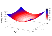
dropping the site energy diagonal terms. The quantities , , represent the lattice parameter lengths along the three crystallographic vectors of the conventional cell. We assume , , . Coropceanu We follow the experimental paper by Ding et al. in order to extract the transfer integrals. Ostrogota The lowest HOMO derived band is measured through ARPES yielding the hopping parameters , , . The dispersion law at is drawn in figure . For small values of and , this graph strictly resembles a paraboloid. It is clear that an effective dispersion law
is capable to fit well the dispersion law (2) for small values of and and . Fit estimates give and . For there is no experimental measure but theoretical estimates seem to agree that it should be small compared with other directions and it is likely owing to the large interplanar separation of rubrene. In the following we assume much smaller than and . As we will discuss later, varying its value seems not too affect much the calculated mobilities.
The electronic part is then
| (3) |
| (4) |
In the last formula () represents the creation (destruction) of a charge carrier in the site , is the bare effective transfer integral in the direction , the el-ph parameter that controls the effect on the transfer integral of the ion displacements in the direction . Once fixed , we impose and, in the same way, .
The dynamic contained in the term is fully quantum, while we remind that the lattice obeys a classical dynamic. This assumption is justified by the adiabatic ratio . Therefore, the results discussed in this paper are valid starting from temperatures such that , with Boltzmann constant. In the adiabatic limit the dimensionless quantity
| (5) |
is the only relevant parameter to quantify the el-ph coupling strength. An ab-initio estimate Troisi Rubrene of has been given for rubrene and it has been substantially confirmed later. Bologna ab-initio ; Bologna Raman This represents our starting point, but a study of the mobility behaviour when raises has been performed and is reported in the following sections. In fact, if is claimed to be a good value for the coupling in one dimension, keeping in mind the increase of the kinetic energy with dimensionality, the equivalent should be higher in three dimensions. Simulations will focus on temperature significantly lower than because this is the typical range investigated experimentally in OFETs. Moreover, in most OFETs the induced charge carrier concentration is rarely higher than and this is the upper limit for the concentrations in our simulations. As shown in a previous paper dealing with a very similar but 1D model, Cataudella SSH-1d for this range of concentrations, the probability distribution of displacements is only slightly renormalized. Therefore, it is acceptable to refer to a free-oscillator (Gaussian) distribution for the displacements:
| (6) |
where is the finite size of the lattice and . We fix (i.e. we consider two crystalline layers) because in OFETs the effective channel of conductions cover very few planes. Shehu Moreover, it is worth reminding that is very small.
We use exact diagonalization to investigate both static and dynamical properties for the hamiltonian (1). At fixed configuration , one has to diagonalize the Hamiltonian yielding eigenvalues , with . The eigenvector components , with , are given through the unitary matrix which diagonalizes the electronic problem. Each observable results from an average on lattice configurations. For example, the electron part of the partition function can be calculated as , where is the quantum partition function of the electron subsystem at a given displacement configuration . Z Monte Carlo Similarly, this would provide approximation-free evaluation of observables such as mobility and spectral function in the semiclassical limit. Observables Monte Carlo The real limitation is the accessible finite size of the lattice. The computing time for each diagonalization is of order and this constraints our analyses up to . In order to reduce the finite size effect, we use periodic boundary conditions. We have checked that, for all the static and dynamic quantities studied in this paper, the thermodynamic limit is reached. The averages are performed by means of a Monte-Carlo procedure. Actually, we generate a sequence of random numbers distributed according to . For the systems investigated in this paper, to get a good accuracy even for dynamic quantities we perform the averages on a number of iterations up to ten thousands.
Within the same framework, it is also possible to calculate the spectral functions, the density of states, and the conductivity. At fixed configuration, the density of states is :
| (7) |
where represents the diagonal term of the spectral function
| (8) |
The spectral function in momentum representation can be determined after performing the averages over the lattice configurations. In the case of conductivity, for each configuration, we calculate the exact Kubo formula Mahan
| (9) | |||||
where , is the Fermi distribution
| (10) |
corresponding to the exact eigenvalue at any chemical potential and is the matrix element of the current operator along the direction , defined as
| (11) |
with electron charge. We notice that, in contrast with spectral properties, the temperature enters the calculation not only through the displacement distribution, but also directly for each configuration through the Fermi distributions . The numerical calculation of the conductivity is able to include the vertex corrections discarded by previous approaches.
Finally, the mobility is defined as
| (12) |
For finite lattice sizes, the delta function appearing in spectral and transport properties has to be replaced with a Lorentzian, thus introducing a finite broadening
| (13) |
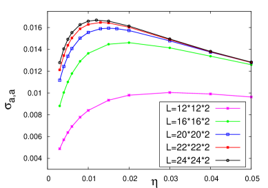
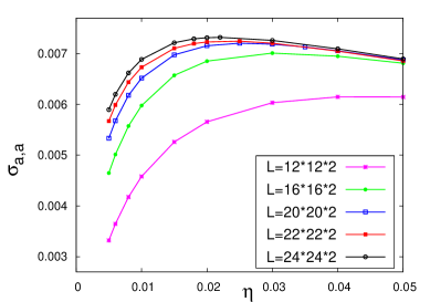
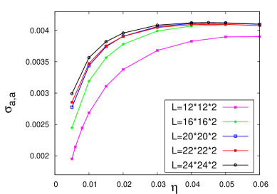
Clearly, the limit procedure means that the value of should be kept as small as possible. This does not give any problem for quantities at finite frequency, as far as . In the case of mobility, this procedure has to be correctly implemented since there is the limit . The correct expression is obtained performing the limits in the following order: , and . These limits are not trivial, so that in the Appendix we have reported in detail the “calibration procedure” followed to fix the right for the calculation of the mobility. In contrast with the 1D case, in our system the mobility dependence on the broadening exhibits a quasi-plateau with a maximum whose location gets closer to the zero as the size of the lattice increases. This makes possible to set as the lowest energy scale of the system. In addition, it emerges quite clearly that, for the sizes considered in this work, the system is very close to the thermodynamic limit. This shows that the broadening is a parameter of the system which does not influence the mobility estimates. A detailed analysis has allowed us to obtain values for and that assure the determination of the correct value of the mobility for any temperature. For the mobilities presented in this paper, we used , of the order of .
In the following, we will measure energies in units of . We will use units such that Boltzmann constant and Planck constant . We will consider the hopping parameters for rubrene derived in this section, therefore . Along the axis, we assume . The small effects due to a change in the value of will be discussed in the end of section about transport properties. Next spectral properties are analyzed.
III Spectral properties
The study of spectral properties is important to individuate the states that mainly contribute to the conduction process. In Fig. 2, the Density Of States (DOS) is shown for different temperatures at and . As shown in logarithmic scale, the DOS has a tail with a low energy exponential behavior. This region corresponds to localized states. economou We have checked analyzing the wave functions extracted from exact diagonalizations that, actually, states with energies deep in the tail are strongly localized (one or two lattice parameters along the different directions as localization length). On the other hand, beyond the shoulder (see Fig. 2 for , and ), the itinerant nature of states is clearly obtained. This analysis gives rough indications for the mobility edge energy which can be located very close to the band edge for free electron (in our case, ).
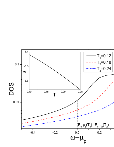
The states available in the tail increase with temperature. It is important to analyze the role played by the chemical potential with varying the temperature. Actually, enters the energy tail and will penetrate into it with increasing temperature. At fixed particle density , for , one has , while, for , (see the inset of Fig. 2). One important point is that the quantity and the close mobility edge are always over . Therefore, in the regime of low density relevant for OFET, the itinerant states are not at but at higher energies. We will show that these states are relevant for the conduction process. Therefore, the analysis of the properties of a high dimensional model points out that both localized and itinerant states are present in the system. This is a clear advantage of our work over previous studies in low dimensionality Troisi Orlandi ; Troisi2D ; Ciuchi Fratini in which there are states that are more localized at very low energy and just less localized close to the free electron edge. Apparently, in our system, with increasing temperature, more localized states become available close to , and so the itinerant states become statistically less effective due to the behavior of the chemical potential. Eventually, the effect of penetration of in the tail will overcome the enlargement of available itinerant states due to the Fermi statistics. We have checked that the trend of the chemical potential towards the energy region of the tail is enhanced with increasing the el-ph coupling .
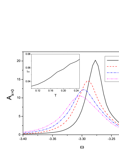
The density of states can be calculated as the sum of the spectral functions over all the momenta . We have checked that the spectral functions with low momentum are more peaked, while, with increasing , they tend to broaden. Perroni Holstein The tail in the DOS is due to a marked width of the high momentum spectral functions. In Fig. 3 we report the spectral function at for the same model parameters as the previous figure. The low damped states close to will keep their itinerant character, and they will be involved into the diffusive conduction process. Actually, we notice that the spectral function gives a negligible contribution to the weight of DOS at the chemical potential for all the temperatures. For example, at , the spectral weight is concentrated in an energy region higher than that in which the chemical potential is located ( for ). Actually, the spectral weight is in the region between and . Finally, we point out that, with increasing temperature, the peak position of the spectral function is only poorly renormalized in comparison with the bare one, in agreement with results of 1D SSH model. Cataudella SSH-1d
It is interesting to estimate the lifetime of the states at low momentum. The spectral functions at shift and broaden with increasing temperature due to the enhanced role of the el-ph coupling. We have estimated the widths at half height in the inset of Fig. 3. At intermediate temperatures, the width is of the order of , that means of the order of . Therefore, the lifetime of these states is of the order of . In the next section, this lifetime will be compared with the transport lifetime derived from the mobility.
The analysis of the spectral properties has clarified important features of the chemical potential and of the states participating at the transport process. Next, we investigate the "transition rules" between states involved into the conduction and analyze the mobility as a function of the particle density and the el-ph coupling.
IV Transport properties
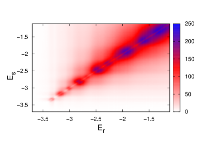
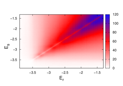
In this section, the focus will be on the Kubo formula for the conductivity given in Eq. (9). We will start from the analysis of the square modulus matrix elements of the current operator along the direction between exact eigenstates and . In Fig. 4, we report the contour plot of the current matrix elements in which the two axes are linked to the energies of the eigenstates. We consider two different temperatures and . The dark color point towards high values of the matrix elements, the bright color to low ones. The difference in the intensity between bright and dark regions correspond to square modulus matrix elements differing for about two orders of magnitude. The most important features emerging from the upper plot is that, in the energy range important for low particle densities, there is a narrow region from about to in which the matrix elements give an appreciable contribution. Moreover, states close in energy do not repel, but have sizable overlapping. These features are clearly ascribed to the role of itinerant states. economou We notice that there are several gaps in the intensities between and , then, very high matrix elements occur going toward the center of the electronic band. At higher temperature (Fig. 4, lower panel), the contour map is broader, the gaps are almost completely removed and the absolute magnitude of the matrix elements is lower. We point out the these "transition rules" are not strongly dependent on the particle density. We stress that, only for density larger than , the matrix elements are sizeable, and the conduction states are far from the tail of the DOS, therefore one would get a "metallic state" typical of an inorganic compound. Indeed, both low density and el-ph interaction contribute to reduce the conducibilities of OFET in comparison with inorganic systems.
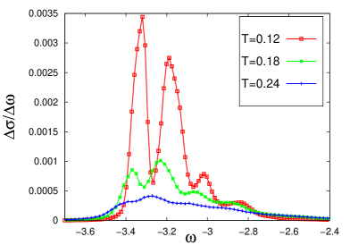
The set of parameters used for the calculation of the mobility are discussed in Appendix A. Before calculating the mobility as a function of the temperature, we analyze the mobility along the direction as a function of the energy of the states which contribute to it. More precisely, in Eq. (9), we sum over the "outgoing states" and analyze the results in terms of the "ingoing states" . We again investigate the regime of low density relevant for OFET. In Fig. 5, we plot as a function of . At low temperature , the "initial" states relevant for the conduction are in the energy range where the current matrix elements are larger, i.e. from about . Furthermore, they are in the range between and , so that they are itinerant. We, finally, note that the curve reproduces the same gaps as showed in Fig. 4. With increasing temperature, the itinerant states become more diffusive and distant from the chemical potential, and, within the energy range close to , more and more localized states are present. This is the reason why the mobility gets lower at room temperature where it is nearly flat as function of the energy.
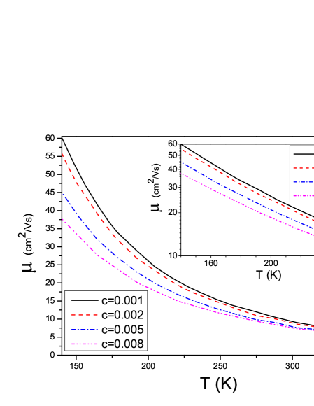
In Fig. (6), the mobility along the direction as a function of the temperature is reported at fixed coupling and for different concentrations . The upper panel shows that the absolute magnitude of the mobility substantially agrees with the experimental estimates being at room temperature, while, in the inset, where the scale is logarithmic, the mobility exhibits a quite linear dependence on the temperature that means a “band-like” behaviour with inverse power-law . The exponent is evaluated as the slope of the straight lines drawn in the lower panel and the results that we obtain from the fit are in the range , where the highest value is related to the lower concentration. This trend is in agreement with experimental measures that for rubrene establish for temperatures . Morpurgo A feature of our model is that the mobility decreases for higher concentrations of carriers. This trend has been already found in the one-dimensional model. Cataudella SSH-1d Actually, due to the "selection rules" discussed previously, increasing density can bring the system into an energy range where the current matrix elements get lower.
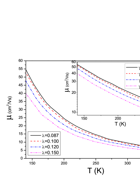
In Fig. (7) the mobility as a function of the temperature is reported at fixed concentration and for different couplings starting from the value . We just notice two essential features emerging from Fig. (7). Quite obviously, the mobility decreases when the coupling strength is higher but, differently from the one-dimensional value which predicts the formation of bond polaron at , Cataudella SSH-1d in this case this does not occur even at higher values of for which the “band-like” behaviour still holds. To conclude this point, we notice that the effect of the coupling on is less relevant then that of the particle density .
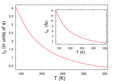
Starting from the mobility, we can determine the scattering time from the relation . Since the mass is weakly renormalized from the el-ph interaction, one can assume as the bare mass at . In the inset of Fig. 8, the scattering time as a function of the temperature is shown. We point out that is on the scale of the , so that it is one order of magnitude lower than the damping time of the states important for the spectral properties (on the scale of ten ). Therefore, the transport processes amplify the effects of the el-ph interaction and the vertex corrections introduced within our approach are fundamental to take into account this effect.
From the scattering time, one can deduce the mean free path as , where is an average velocity of the charge carriers. We estimate from the average kinetic energy as follows:
| (14) |
The operator has to be intended both as a thermic average and as an average over the configurations . The quantity is reported in Fig. 8. It is always on the scale of a few lattice parameters. The most important feature is its temperature behavior. As a consequence of the el-ph interaction effects, close to room temperature, it becomes of the order of half lattice parameter . This means that the Ioffe-Regel limit is reached. Gunnarsson The decrease of the mobility in the Ioffe-Regel limit is not due to a mass renormalization (dynamic and/or static) but is due to a reduction of the available itinerant states (the only ones able to transport current) with the temperature. We remark that this result is due to the fundamental role played by vertex corrections in the calculation of the mobility.
Another important quantity is the anisotropy of the transport properties along different in-plane directions. Up to now, we have discussed the mobility only along the direction, since the corresponding quantity along the axis can be roughly reproduced taking into account the anisotropy factors . Actually, the mobility along direction roughly scales as the square of the ratio , therefore it is about times the mobility along the direction. This value is in good agreement with experimental results. Morpurgo
Finally, we briefly discuss the role of hopping parameter on the mobility features. Switching from to produces a relative reduction of the mobility that lies between and depending on the concentration of carriers . Although the sensitivity of the mobility to is less relevant than other parameters, can’t properly be treated as a “dead parameter”. There may be two reasons for this effect: first reducing the interplanar coupling yields to a system more bidimensional and many theoretical predictions state that a purely bidimensional system should be an insulator, economou then, when becomes comparable with the broadening (we keep in the range , see Appendix) the finiteness of the lattice appears partially invalidating the procedure. Probably, both effects give their contribution to the reduction of the mobility.
V Summary and conclusions
Spectral and transport properties of the quasi two-dimensional adiabatic Su-Schrieffer-Heeger model have been discussed with reference to rubrene single-crystal field effect transistors. An important ingredient of our model is the small but finite carrier density, therefore the interesting behavior of the chemical potential as function of temperature has been investigated. Actually, with increasing temperature, the chemical potential always enters the tail of the density of states corresponding to localized states. Therefore, all the experimentally quantities strongly dependent on the position of the chemical position will probe the features of localized states. The combined study of spectral and transport properties is fundamental to shed light on the intricate conduction process of these materials characterized by small particle density and intermediate el-ph coupling. From this analysis it emerges that the states that mainly contribute to the conduction process are the itinerant ones which are in the energy range between and . With increasing temperature, these states are affected by enhanced interaction effects and are more distant from , and, at the same time, more and more localized states become available in the energy range close to the chemical potential. Therefore, close to room temperature, the transport properties reach the Ioffe-Regel limit. Moreover, the transport lifetime is almost one order of magnitude smaller than the spectral lifetime of the states involved in the transport mechanism. In order to get this result, it is important to include vertex corrections into the calculation of the mobility. The mobility as a function of temperature is in good agreement with experiments: indeed, the mobility has the right order of magnitude, it scales as a power law , with the close or larger than two, and has the correct anisotropy ratio between different in-plane directions. The use of a realistic quasi 2D model is fundamental for the analysis of this paper providing reliable results.
The focus of this work has been on the effects of low frequency intermolecular modes on the transport properties. While the mobility from to is believed to depend almost entirely by this el-ph coupling, close to room temperature, the effects of other interactions, for example that due to local high frequency modes, can give a non negligible contribution. Perroni_Comb Actually, when the mean free path becomes of the order of the lattice parameter as a result of the only intermolecular coupling, the local coupling can easily give rise to an hopping mechanism with an activated mobility. Rubrene is on the verge of this behavior, that can be accepted as a mechanism for other poliacenes. As a future work, it could be interesting to use the quasi 2D model discussed in this paper in combination with local el-ph coupling in order to better understand the conduction mechanism close to room temperature. Work in this direction is in progress.
Appendix A “Calibration procedure”
In this Appendix, we report in detail the “calibration procedure” followed to fix the right value of the broadening for the calculation of the mobility. According to Eqs. (12) and (13), the mobility is obtained performing the two limits and together with thermodynamic limit . It is clear that the limit on the size and on has to be done at the same time because, actually, they are similar. Moreover, it turns out that, for any fixed choice of the couple and for any temperature , the mobility depends slightly on the frequency . There is a threshold under which the mobility is not sensitive to further decreasing of that means that we have reached the minimum frequency that our finite system can resolve. Practically, under the value the mobility shows a plateau. We have fixed this value for all the calculations of mobility.
In Fig. (9), for three different values of temperature, we have plotted the mobility calculated via the Kubo formula (9) to analyze how it depends on and the size . The strength of coupling is fixed at and the carrier concentration is . At any temperature, the series of data gets closer with increasing the size of the lattice. Eventually, for the two biggest sizes, they are not distinguishable for most of the range in which varies. This allows us to state that, for the maximum size that we can treat , the system actually reaches the thermodynamic limit or at least gets very close to it. For example, in the worst case of low temperature ( equivalent to ) the two upper curves split only for and it is clear that the value for which the highest mobility is reached gets closer to zero as the size rises. For all the regimes of temperature, the mobility exhibits a quasi-plateau (less definite at low temperatures) and the value of under which the mobility collapses is reduced by increasing the size. This trend can be easily explained if one notices that, when the size increases, the separation between two next eigenvalues reduces and the same happens to the width of the delta function required to couple a proper number of close eigenvalues. Another feature that is worth to be noticed is that the curves of different sizes merge together in better way at high temperatures then at low ones but, at the same time, for high temperatures is higher. These arguments lead us to state that, for our model, a correct thermodynamic limit can be recovered in spite of the analogue 1D model in which the mobility falls down under a value of that in the limit of infinite size converges on a finite . Cataudella SSH-1d . It seems that in 1D the broadening is not just a computational need that virtually disappears in the infinite size limit but it’s a real missing energy scale without which a finite mobility can’t be obtained. Operatively, for each of the three temperature that appear in Fig. (9), we have determined the value for which the mobility has a maximum. Then, at any intermediate temperature , the is obtained from a quadratic interpolation based on . This procedure allows to calculate a mobility very close to that one reached in the thermodynamic limit.
References
- (1) T. Hasegawa and J. Takeya, Sci. Technol. Adv. Mater. 10, 24314 (2009).
- (2) M. E. Gershenson, V. Podzorov and A. F. Morpurgo, Rev. Mod. Phys. 78, 973 (2006).
- (3) Y. C. Cheng, R. J. Silbey, D. A. da Silva Filho, J. P. Calbert, J. Cornil, and J. L. Bredas, J. Chem. Phys. 118 3764 (2003).
- (4) H. Ding, C. Reese, A. J. Makinen, Z. Bao, and Y. Gao, Appl. Phys. Lett. 96, 222106 (2010).
- (5) S. I. Machida, Y. Nakayama, S. Duhm, Q. Xin, A. Funakoshi, N. Ogawa, S. Kera, N. Ueno, and H. Ishii, Phys. Rev. Lett. 104, 156401 (2010).
- (6) K. Marumoto, S. Kuroda, T. Takenobu, and Y. Iwasa, Phys. Rev. Lett. 97, 256603 (2006).
- (7) K. Marumoto, N. Arai, H. Goto, M. Kijima, K. Murakami, Y. Tominari, J. Takeya, Y. Shimoi, H. Tanaka, S. Kuroda, T. Kaji, T. Nishikawa, T. Takenobu, and Y. Iwasa, Phys. Rev. B 83, 075302 (2011).
- (8) H. A. V. Laarhoven, C. F. J. Flipse, M. Koeberg, M. Bonn, E. Hendry, G. Orlandi, O. D. Jurchescu, T.T.M. Palstra, and A. Troisi, J. Chem. Phys. 129, 044704 (2008).
- (9) T. Sakanoue and H. Sirringhaus, Nat. Mater. 9 736 (2010).
- (10) V. Coropceanu, J. Cornil, D. A. da Silva Filho, Y. Oliver, R. Silbey and J. L. Bredas, Chem. Rev. 107, 926 (2007).
- (11) A. Troisi and G. Orlandi, Phys. Rev. Lett. 96, 222106 (2006).
- (12) W. P. Su, J. R. Schrieffer and A. J. Heeger, Phys. Rev. Lett 42, 1698 (1979).
- (13) A. Troisi, Adv. Mat 19, 2000 (2007).
- (14) A. Troisi, J. Chem. Phys. 134, 034702 (2011).
- (15) A. Madhukar and W. Post, Phys. Rev. Lett. 39, 1424 (1977).
- (16) S. Fratini and S.Ciuchi, Phys. Rev. Lett. 103, 266601 (2009).
- (17) P. W. Anderson, Phys. Rev. 109, 1492 (1958).
- (18) V. Cataudella, G. De Filippis and C. A. Perroni, Phys. Rev. B 83, 165203 (2010).
- (19) C. A. Perroni, A. Nocera, V. Marigliano Ramaglia, and V. Cataudella, Phys. Rev. B 83, 245107 (2011).
- (20) T. Holstein, Ann. Phys. 10 325 (1959).
- (21) T. Holstein, Ann. Phys. 10 343 (1959).
- (22) A. Girlando, L. Grisanti, and M. Masino, Phys. Rev. B 82, 035208 (2010).
- (23) E. Venuti, I. Billotti, R. G. Della Valle, A. Brillante, P. Ranzieri, M. Masino and A. Girlando, J. Phys. Chem. C 112, 17416 (2008).
- (24) A. Shehu, S. D. Quiroga, P. D’Angelo, C. Albonetti, F. Borgatti, M. Murgia, A. Scorzoni, P. Stoliar, and F. Biscarini, Phys. Rev. Lett. 104, 246602 (2010).
- (25) K. Michielsen and H. de Raedt, Mod. Phys. Lett. B, 10, 467 (1996)
- (26) E. Dagotto, T. Hotta, A. Moreo, Phys. Rep. 344, 153 (2001).
- (27) G. D. Mahan, Many-Particle Physics, 2nd ed. (Plenum Press, New York, 1990).
- (28) E. N. Economou, Green’s Functions in Quantum Physics (Springer Verlag, Berlin, 1983).
- (29) O. Gunnarson, M. Calandra, and J. E. Han, Rev. Mod. Phys. 73, (2003).
- (30) C. A. Perroni, V. Marigliano Ramaglia, and V. Cataudella, Phys. Rev. B 84, 014303 (2011).