Energy estimates and cavity interaction for a critical-exponent cavitation model

Abstract

We consider the minimization of $\int_{\Omega_{\varepsilon}}|D\mathbf{u}|^{p}\,\mathrm{d}\mathbf{x}$ in a perforated domain $\Omega_{\varepsilon}:=\Omega\setminus\bigcup_{i=1}^{M}B_{\varepsilon}(\mathbf{a}_{i})$ of $\mathbb{R}^{n}$, among maps $\mathbf{u}\in W^{1,p}(\Omega_{\varepsilon},\mathbb{R}^{n})$ that are incompressible ($\det D\mathbf{u}\equiv 1$), invertible, and satisfy a Dirichlet boundary condition $\mathbf{u}=\mathbf{g}$ on $\partial\Omega$. If the volume enclosed by $\mathbf{g}(\partial\Omega)$ is greater than $|\Omega|$, any such deformation $\mathbf{u}$ is forced to map the small holes $B_{\varepsilon}(\mathbf{a}_{i})$ onto macroscopically visible cavities (which do not disappear as $\varepsilon\to 0$). We restrict our attention to the critical exponent $p=n$, where the energy required for cavitation is of the order of $\sum_{i=1}^{M}v_{i}|\log\varepsilon|$ and the model is suited, therefore, for an asymptotic analysis ($v_{1},\ldots,v_{M}$ denote the volumes of the cavities). In the spirit of the analysis of vortices in Ginzburg-Landau theory, we obtain estimates for the “renormalized” energy $\frac{1}{n}\int_{\Omega_{\varepsilon}}\left|\frac{D\mathbf{u}}{\sqrt{n-1}}\right|^{p}\,\mathrm{d}\mathbf{x}-\sum_{i}v_{i}|\log\varepsilon|$, showing its dependence on the size and the shape of the cavities, on the initial distance between the cavitation points $\mathbf{a}_{1},\ldots,\mathbf{a}_{M}$, and on the distance from these points to the outer boundary $\partial\Omega$. Based on those estimates we conclude, for the case of two cavities, that either the cavities prefer to be spherical in shape and well separated, or to be very close to each other and appear as a single equivalent round cavity. This is in agreement with existing numerical simulations, and is reminiscent of the interaction between cavities in the mechanism of ductile fracture by void growth and coalescence.

1 Introduction

1.1 Motivation

In nonlinear elasticity, cavitation is the name given to the sudden formation of cavities in an initially perfect material, due to its incompressibility (or near-incompressibility), in response to a sufficiently large and triaxial tension. It plays a central role in the initiation of fracture in metals [35, 62, 34, 78, 58] and in elastomers [29, 80, 32, 22, 18] (especially in reinforced elastomers [57, 31, 15, 9, 52]), via the mechanism of void growth and coalescence. It has important applications such as the indirect measurement of mechanical properties [45] or the rubber-toughening of brittle polymers [46, 14, 76, 48]. Mathematically, it constitutes a realistic example of a regular variational problem with singular minimizers, and corresponds to the case when the stored-energy function of the material is not $W^{1,p}$-quasiconvex [2, 5, 7], the Jacobian determinant is not weakly continuous [7], and important properties such as the invertibility of the deformation may not pass to the weak limit [55, Sect. 11]. The problem has been studied by many authors, beginning with Gent-Lindley [30] and Ball [4]; see the review papers [29, 41, 25], the variational models of Müller-Spector [55] and Sivaloganathan-Spector [70], and the recent works [38, 49] for further motivation and references.

The standard model in the variational approach to cavitation considers functionals of the form

$$\int_{\Omega}|D\mathbf{u}|^{p}\,\,\mathrm{d}\mathbf{x},$$ (1.1)

where the deformation $\mathbf{u}:\Omega\subset\mathbb{R}^{n}\to\mathbb{R}^{n}$ is constrained to be incompressible (i.e. $\det D\mathbf{u}=1$) and globally invertible, and either a Dirichlet condition $\mathbf{u}=\mathbf{g}$ or a force boundary condition is applied. Unless the boundary condition is exactly compatible with the volume, cavities have to be formed. If $p<n$ this can happen while still keeping a finite energy. A typical deformation creating a cavity of volume $\omega_{n}A^{n}$ at the origin ($\omega_{n}$ being the volume of the unit ball in $\mathbb{R}^{n}$) is given by

$$\mathbf{u}(\mathbf{x})=\sqrt[n]{A^{n}+|\mathbf{x}|^{n}}\frac{\mathbf{x}}{|\mathbf{x}|}.$$ (1.2)

We can easily compute that

$$|D\mathbf{u}|^{2}\mathop{\sim}_{\mathbf{x}=\mathbf{0}}\frac{(n-1)A^{2}}{|\mathbf{x}|^{2}}.$$ (1.3)

In that situation the origin is called a cavitation point, which belongs to the domain space, and its image by $\mathbf{u}$ is the cavity, belonging to the target space. Contrarily to the usual, we study the critical case $p=n$ where the cavity behaviour (1.2) just fails to be of finite energy.

This fact is analogous to what happens for $\mathbb{S}^{1}$-valued harmonic maps in dimension 2, which were particularly studied in the context of the Ginzburg-Landau model, see Bethuel-Brezis-Hélein [10]. For $\mathbb{S}^{1}$-valued maps $\mathbf{u}$ from $\Omega\subset\mathbb{R}^{2}$, the topological degree of $\mathbf{u}$ around a point $\mathbf{a}$ is defined by the following integer

$$d=\frac{1}{2\pi}\int_{\partial B(\mathbf{a},r)}\frac{\partial\mathbf{u}}{\partial\tau}\times\mathbf{u}.$$

Points around which this is not zero are called vortices. Typical vortices of degree $d$ look like $\mathbf{u}=e^{id\theta}$ (in polar coordinates). If $d\neq 0$ again $|D\mathbf{u}|^{2}$ just fails to be integrable since for the typical vortex $|D\mathbf{u}|^{2}\sim_{\mathbf{x}=\mathbf{0}}\frac{|d|^{2}}{|\mathbf{x}|^{2}}$, just as above (1.3), up to a constant factor. So there is an analogy in that sense between maps from $\Omega$ to $\mathbb{C}$ which are constrained to satisfy $|\mathbf{u}|=1$, and maps from $\Omega$ to $\mathbb{R}^{2}$ which satisfy the incompressibility constraint $\det D\mathbf{u}=1$. We see that in this analogy (in dimension 2) the volume of the cavity divided by $\pi$ plays the role of the absolute value of the degree for $\mathbb{S}^{1}$-valued maps. In this correspondence two important differences appear: the degree is quantized while the cavity volume is not; on the other hand the degree has a sign, which can lead to “cancellations” between vortices, while the cavity volume is always positive.

In the context of $\mathbb{S}^{1}$-valued maps, two possible ways of giving a meaning to $\int_{\Omega}|D\mathbf{u}|^{2}$ are the following. The first is to relax the constraint $|\mathbf{u}|=1$ and replace it by a penalization, and study instead

$$\int_{\Omega}|D\mathbf{u}|^{2}+\frac{1}{\varepsilon^{2}}(1-|\mathbf{u}|^{2})^{2}$$ (1.4)

in the limit $\varepsilon\to 0$; this is the Ginzburg-Landau approximation. The second is to study the energy with the constraint $|\mathbf{u}|=1$ but in a punctured domain $\Omega_{\varepsilon}:=\Omega\backslash\cup_{i}B({\mathbf{a}}_{i},\varepsilon)$ where ${\mathbf{a}}_{i}$’s stand for the vortex locations:

$$\min_{|\mathbf{u}|=1}\int_{\Omega_{\varepsilon}}|D\mathbf{u}|^{2}$$ (1.5)

again in the limit $\varepsilon\to 0$; this can be called the “renormalized energy approach”. Both of these approaches were followed in [10], where it is proven that the Ginzburg-Landau approach essentially reduces to the renormalized energy approach. More specifically, when there are vortices at ${\mathbf{a}}_{i}$, $|D\mathbf{u}|$ will behave like $|d_{i}|/|\mathbf{x}-{\mathbf{a}}_{i}|$ near each vortex (where $d_{i}$ is the degree of the vortex) and both energies (1.4) and (1.5) will blow up like $\pi\sum_{i}d_{i}^{2}\log\frac{1}{\varepsilon}$ as $\varepsilon\to 0$. It is shown in [10] that when this divergent term is subtracted off (this is the “renormalization” procedure), what remains is a nondivergent term depending on the positions of the vortices ${\mathbf{a}}_{i}$ and their degrees $d_{i}$ (and the domain), called precisely the renormalized energy. That energy is essentially a Coulombian interaction between the points ${\mathbf{a}}_{i}$ behaving like charged particles (vortices of same degree repel, those of opposite degrees attract) and it can be written down quite explicitly.

Our goal here is to study cavitation in the same spirit. A first attempt, which would be the analogue of (1.4), would be to relax the incompressibility constraint and study for example

$$\int_{\Omega}|D\mathbf{u}|^{2}+\frac{(1-\det D\mathbf{u})^{2}}{\varepsilon}.$$ (1.6)

We do not however follow this route which seems to present many difficulties (one of them is that this energy in two dimensions is scale invariant, and that contrarily to (1.4) the nonlinearity contains as many order of derivatives as the other term), but it remains a seemingly interesting open problem, which would have good physical sense. Rather we follow the second approach, i.e. that of working in punctured domains while keeping the incompressibility constraint.

For the sake of generality we consider holes which can be of different radii $\varepsilon_{1},\cdots,\varepsilon_{m}$, define $\Omega_{\varepsilon}:=\Omega\backslash\cup_{i=1}^{m}\overline{B}(\mathbf{a}_{i},\varepsilon_{i})$ and look at

$$\min_{\det D\mathbf{u}=1}\int_{\Omega_{\varepsilon}}|D\mathbf{u}|^{2}$$ (1.7)

(or $\min_{\det D\mathbf{u}=1}\int_{\Omega_{\varepsilon}}|D\mathbf{u}|^{n}$ in dimension $n$), in the limit $\varepsilon\to 0$. This also has a reasonable physical interpretation: it corresponds to studying the incompressible deformation of a body that contains micro-voids which expand under the applied boundary deformation. One may think of the points ${\mathbf{a}}_{i}$ as fixed, then they correspond to defects that pre-exist, just as above. Or the model can be seen as a fracture model where we postulate that the body will first break around the most energetically favorable points ${\mathbf{a}}_{i}$ (see, e.g., the discussion in [4, 43, 69, 29, 42, 55, 6, 71, 74, 49, 50]). It can also be compared to the core-radius approach in dislocation models [13, 59, 28].

Following the analogy above, we would like to be able to subtract from (1.7) a leading order term proportional to $\log\frac{1}{\varepsilon}$, in order to extract at the next order a “renormalized” term which will tell us how cavities “interact” (attract or repel each other), according to their positions and shapes. This is more difficult than the problem (1.5) because the condition $\det D\mathbf{u}=1$ is much less constraining than $|\mathbf{u}|=1$. While the maps with $|\mathbf{u}|=1$ can be parametrized by lifting in the form $\mathbf{u}=e^{i\varphi}$, to our knowledge no parametrization of that sort exists for incompressible maps. In addition while the only characteristic of a vortex is an integer –its degree–, for incompressible maps, the characteristics of a cavity are more complex –they comprise the volume of the cavity and its shape–, and there is no quantization. For these reasons we cannot really hope for something as nice and explicit as a complete “renormalized energy” for this toy cavitation model. However we will show that we can obtain, in particular in the case of two cavities, some quantitative information about the cavities interaction that is reminiscent of the renormalized energy.

1.2 Method and main results : energy lower bounds

Our method relies on obtaining general and ansatz-free lower bounds for the energy on the one hand, and on the other hand upper bounds via explicit constructions, which match as much as possible the lower bounds. This is in the spirit of $\Gamma$-convergence (however we will not prove a complete $\Gamma$-convergence result). For simplicity in this section we present the results in dimension 2, but they carry over in higher dimension.

To obtain lower bounds we use the “ball construction method”, which was introduced in the context of Ginzburg-Landau by Jerrard [44] and Sandier [65, 66]. The crucial estimate for Ginzburg-Landau, or more simply $\mathbb{S}^{1}$-valued harmonic maps, is the following simple relation, corollary of Cauchy-Schwarz:

$$\int_{\partial B(\mathbf{a},r)}|D\mathbf{u}|^{2}\geq\frac{1}{2\pi r}\left(\int_{\partial B(\mathbf{a},r)}\frac{\partial\mathbf{u}}{\partial\tau}\times\mathbf{u}\right)^{2}=2\pi\frac{d^{2}}{r}$$ (1.8)

if $d$ is the degree of the map on $\partial B(\mathbf{a},r)$. Integrating this relation over $r$ ranging from $\varepsilon$ to $1$ yields a lower bound for the energy on annuli, with the logarithmic behavior stated above. One sees that the equality case in (1.8) is achieved when $\mathbf{u}$ is exactly radial (which corresponds to $\mathbf{u}=e^{id\theta}$ in polar coordinates), so the least energetically costly vortices are the radial ones. For an arbitrary number of vortices the “ball construction” à la Jerrard and Sandier allows to paste together the lower bounds obtained on disjoint annuli. Previous constructions for bounded numbers of vortices include those of Bethuel-Brezis-Hélein [10] and Han-Shafrir [36]. The ball construction method will be further described in Section 3.1.

For the cavitation model, there is an analogue to the above calculation, which is also our starting point. Assume that $\mathbf{u}$ develops a cavity of volume $v$ around a cavitation point $\mathbf{a}$ in the domain space. By $v$ we really denote the excess of volume created by the cavity (we still refer to it as cavity volume), this way the image of the ball $B(\mathbf{a},\varepsilon)$ contains a volume $\pi\varepsilon^{2}+v$. Using the Cauchy-Schwarz inequality, we may write

$$\int_{\partial B(\mathbf{a},r)}|D\mathbf{u}|^{2}\geq\frac{1}{2\pi r}\left(\int_{\partial B(\mathbf{a},r)}|D\mathbf{u}\cdot\tau|\right)^{2}.$$ (1.9)

But then one can observe that $\int_{\partial B(\mathbf{a},r)}|D\mathbf{u}\cdot\tau|$ is exactly the length of the image curve of the circle $\partial B(\mathbf{a},r)$. We may then use the classical isoperimetric inequality

$$(\operatorname{Per}E(\mathbf{a},r))^{2}\geq 4\pi|E(\mathbf{a},r)|$$ (1.10)

where $|\cdot|$ denotes the volume, and $E(\mathbf{a},r)$ is the region enclosed by this image curve, which contains the cavity, and has volume $\pi r^{2}+v$ by incompressibility. Inserting this into (1.9), we are led to

$$\int_{\partial B(\mathbf{a},r)}\frac{|D\mathbf{u}|^{2}}{2}\geq\frac{\operatorname{Per}^{2}(E(\mathbf{a},r))}{4\pi r}\geq\frac{|E(\mathbf{a},r)|}{r}\geq\frac{v}{r}+\pi r.$$ (1.11)

This is the building block that we will integrate over $r$ and insert into the ball construction, to obtain our first lower bound, which is proved in Section 3.1. To state it, we will use the notion of weak determinant:

$$\langle\operatorname{Det}D\mathbf{u},\phi\rangle:=-\frac{1}{n}\int_{\Omega}\mathbf{u}(\mathbf{x})\cdot(\operatorname{cof}D\mathbf{u}(\mathbf{x}))D\phi(\mathbf{x})\,\mathrm{d}\mathbf{x},\qquad\forall\,\phi\in C_{c}^{\infty}(\Omega)$$

whose essential features we recall in Section 2.4; as well as Müller and Spector’s invertibility “condition INV” [55] which is defined in Section 2.3 (Definition 5) and which essentially means that the deformations of the material, in addition to being one-to-one, cannot create cavities which would at the same time be filled by material coming from elsewhere. Even though we have discussed dimension 2, we directly state the result in dimension $n$.

Proposition 1.1.

Let $\Omega$ be an open and bounded set in $\mathbb{R}^{n}$, and $\Omega_{\varepsilon}=\Omega\backslash\cup_{i=1}^{m}\overline{B}({\mathbf{a}}_{i},\varepsilon_{i})$ where ${\mathbf{a}}_{1},\cdots,{\mathbf{a}}_{m}\in\Omega$ and the $\overline{B}({\mathbf{a}}_{i},\varepsilon_{i})$ are disjoint. Suppose that $\mathbf{u}\in W^{1,n}(\Omega_{\varepsilon},\mathbb{R}^{n})$ and that condition INV is satisfied. Suppose, further, that $\operatorname{Det}D\mathbf{u}=\mathcal{L}^{n}$ in $\Omega_{\varepsilon}$ (where $\mathcal{L}^{n}$ is the Lebesgue measure), and let $v_{i}:=|E({\mathbf{a}}_{i},\varepsilon_{i})|-\omega_{n}\varepsilon_{i}^{n}$ (with $E(\mathbf{a}_{i},\varepsilon_{i})$ as in (1.10)). Then for any $R>0$

$$\frac{1}{n}\int_{\Omega_{\varepsilon}}\left(\left|\frac{D\mathbf{u}}{\sqrt{n-1}}\right|^{n}-1\right)\,\mathrm{d}\mathbf{x}\geq\left(\sum_{i,B(\mathbf{a}_{i},R)\subset\Omega}^{m}v_{i}\right)\log\frac{R}{2\sum_{i=1}^{m}\varepsilon_{i}}.$$

Note that $\sum_{i}v_{i}=V$ is the total cavity volume, which due to incompressibility is completely determined by the Dirichlet data, in the case of a displacement boundary value problem.

Examining the equality cases in the chain of inequalities (1.9)–(1.11) already tells us that the minimal energy is obtained when “during the ball construction” all circles (at least for $r$ small) are mapped into circles and the cavities are spherical. A more careful examination of (1.9) indicates that the map should at least locally follow the model cavity map (1.2). It is the same argument that has been used by Sigalovanathan and Spector [72, 73] to prove the radial symmetry of minimizers for the model with power $p<n$.

When there is more than one cavity, and two cavities are close together, we can observe that there is a geometric obstruction to all circles “of the ball construction” being mapped into circles. This is true for any number of cavities larger than 1; to quantify it is in principle possible but a bit inextricable for more than 2. For that reason and for simplicity, we restrict to the case of two cavities, and now explain the quantitative point.

Figure 1: Ball construction in the reference configuration

Let $\mathbf{a}_{1}$ and $\mathbf{a}_{2}$ be the two cavitation points with $|\mathbf{a}_{1}-\mathbf{a}_{2}|=d$, small compared to $1$. For simplicity of the presentation let us also assume that $\varepsilon_{1}=\varepsilon_{2}=\varepsilon$. The ball construction is very simple in such a situation: three disjoint annuli are constructed, $B({\mathbf{a}}_{1},d/2)\backslash B({\mathbf{a}}_{1},\varepsilon)$, $B({\mathbf{a}}_{2},d/2)\backslash B({\mathbf{a}}_{2},\varepsilon)$ and $B(\mathbf{a},R)\backslash B(\mathbf{a},d)$, where $\mathbf{a}$ is the midpoint of ${\mathbf{a}}_{1}$ and ${\mathbf{a}}_{2}$ (see Figure 1). These annuli can be seen as a union of concentric circles centred at ${\mathbf{a}}_{1}$, ${\mathbf{a}}_{2}$, $\mathbf{a}$ respectively. To achieve the optimality condition above, each of these circles would have to be mapped by $\mathbf{u}$ into a circle. If this were true, the images of $B({\mathbf{a}}_{1},d/2)$ and $B({\mathbf{a}}_{2},d/2)$ would be two disjoint balls containing the two cavities, call them $E_{1}$ and $E_{2}$. By incompressibility, $|E_{1}|=v_{1}+\pi(d/2)^{2}$ and $|E_{2}|=v_{2}+\pi(d/2)^{2}$. Then the image of $B(\mathbf{a},d)$ would also have to be a ball, call it $E$, which contains the disjoint union $E_{1}\cup E_{2}$, and by incompressibility

$$|E|=v_{1}+v_{2}+\pi d^{2}.$$ (1.12)

If $d$ is small compared to $v_{1}$ and $v_{2}$ it is easy to check this is geometrically impossible: the radius of the ball $E_{1}$ is certainly bigger than $\sqrt{v_{1}/\pi}$, that of $E_{2}$ than $\sqrt{v_{2}/\pi}$ and since $E$ is a ball that contains their disjoint union, its radius is at least the sum of the two, hence $|E|\geq(\sqrt{v_{1}}+\sqrt{v_{2}})^{2}$. This is incompatible with (1.12) unless $\pi d^{2}\geq 2\sqrt{v_{1}v_{2}}$.

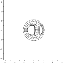
(a) $\mu=0.5$

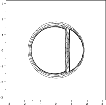
(b) $\mu=1.5$

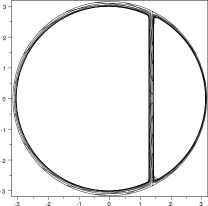
(c) $\mu=3$

Figure 2: Incompressible deformation $\mathbf{u}:B(\mathbf{0},d)\setminus\{\mathbf{a}_{1},\mathbf{a}_{2}\}\to\mathbb{R}^{2}$, $d=|\mathbf{a}_{2}-\mathbf{a}_{1}|$, opening distorted cavities of volumes $v_{1}+\pi\varepsilon_{1}^{2}$, $v_{2}+\pi\varepsilon_{2}^{2}$; deformed configuration for increasing values of the displacement load ($\mu:=\sqrt{\frac{v_{1}+v_{2}}{\pi d^{2}}}$). Choice of parameters: $d=1$, $\frac{v_{2}}{v_{1}}=0.3$.

So in practice, if $d$ is small compared to the volumes, the circles are not all mapped to exact circles, the inclusion and disjointness are preserved, but some distortion in the shape of the images has to be created either for the “balls before merging” i.e. $E_{1}$ and $E_{2}$ – this corresponds to what is sketched on Figure 2 – or for the “balls after merging” i.e. $E$ – this corresponds to what is sketched in Figure 3 (the situations of Figures 2 and 3 correspond to the test-maps we will use to get energy upper bounds, see below Section 1.3).

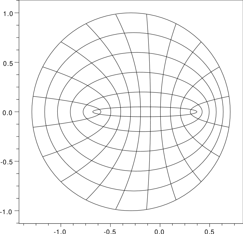
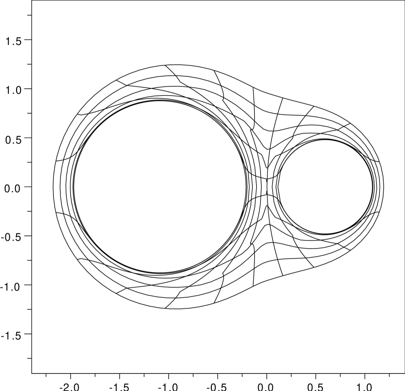
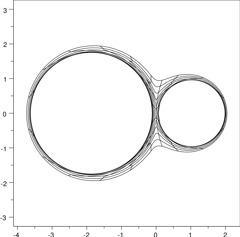
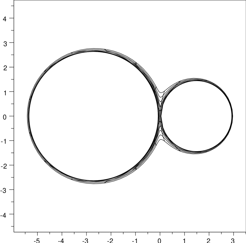
(a) Reference configuration

(b)  Deformed configuration, $\mu=1$

(c) Deformed configuration, $\mu=2$

(d) Deformed configuration, $\mu=3$

Figure 3: Incompressible deformation of $B(\mathbf{0},d)$, $d:=|\mathbf{a}_{2}-\mathbf{a}_{1}|$, for increasing values of $\mu:=\sqrt{\frac{v_{1}+v_{2}}{\pi d^{2}}}$. Final cavity volumes $v_{1}$ and $v_{2}$ given by $d=1$, $\frac{v_{2}}{v_{1}}=0.3$.

A convenient tool to quantify how much these sets differ from balls, which is what we exactly mean by “distortion”, is the following

Definition 1.

The Fraenkel asymmetry of a measurable set $E\subset\mathbb{R}^{n}$ is defined as

$$D(E):=\min_{\mathbf{x}\in\mathbb{R}^{n}}\frac{|E\triangle B(\mathbf{x},r_{E})|}{|E|},\quad\text{with}\ r_{E}\ \text{such that}\ |B(\mathbf{x},r_{E})|=|E|$$

where $\triangle$ denotes the symmetric difference between sets.

Note that $D(E)$ is a scale-free quantity which depends not on the size of $E$, but on its shape.

The following proposition, which we shall prove in Section 3.3, allows to make the observations above quantitative in terms of the distortions.

Proposition 1.2.

Let $E$, $E_{1}$, and $E_{2}$ be sets of positive measure in $\mathbb{R}^{n}$, $n\geq 2$ such that $E\supset E_{1}\cup E_{2}$ and $E_{1}\cap E_{2}=\varnothing$, and assume without loss of generality that $|E_{1}|\geq|E_{2}|$. Then

$$\frac{|E|D(E)^{\frac{n}{n-1}}+|E_{1}|D(E_{1})^{\frac{n}{n-1}}+|E_{2}|D(E_{2})^{\frac{n}{n-1}}}{|E|+|E_{1}\cup E_{2}|}\\ \geq C_{n}\left(\frac{|E_{2}|}{|E_{1}|+|E_{2}|}\right)^{\frac{n}{n-1}}\left(\frac{(|E_{1}|^{\frac{1}{n}}+|E_{2}|^{\frac{1}{n}})^{n}-|E|}{(|E_{1}|^{\frac{1}{n}}+|E_{2}|^{\frac{1}{n}})^{n}-|E_{1}\cup E_{2}|}\right)^{\frac{n(n+1)}{2(n-1)}}$$

for some constant $C_{n}>0$ depending only on $n$.

The fact that $E_{1},E_{2},E$ cannot simultaneously be balls is made explicit by the fact that $D(E_{1})$, $D(E_{2})$, $D(E)$ cannot all vanish unless the right-hand side is negative, which can happen only if $|E|$ is large relative to $|E_{1}|$ and $|E_{2}|$. The first factor in the estimate degenerates only when one of the sets is very small compared to the other.

Note that such a geometric constraint is also true for more than two merging balls, so in principle we could treat (with more effort) the case of more than two cavities, however the estimates would degenerate as the number of cavities gets large.

These estimates on the distortions are useful for us thanks to the following improved isoperimetric inequality, precisely expressed in terms of the Fraenkel asymmetry:

Proposition 1.3 (Fusco-Maggi-Pratelli [27]).

For every Borel set $E\subset\mathbb{R}^{n}$

$$\operatorname{Per}E\geq n\omega_{n}^{\frac{1}{n}}|E|^{\frac{n-1}{n}}(1+CD(E)),$$

where $C$ is a universal constant.

In dimension 2, we thus have the improved isoperimetric inequality

$$(\operatorname{Per}E)^{2}\geq 4\pi|E|+C|E|D^{2}(E),$$ (1.13)

for some universal $C>0$. Inserting (1.13) instead of (1.10) into the basic estimate (1.11) gives us

$$\int_{\partial B(\mathbf{a},r)}\frac{|D\mathbf{u}|^{2}}{2}\geq\frac{|E(\mathbf{a},r)|}{r}+\frac{C}{r}|E(\mathbf{a},r)|D^{2}(E(\mathbf{a},r))\geq\frac{v}{r}+\pi r+\frac{C}{r}|E(\mathbf{a},r)|D^{2}(E(\mathbf{a},r)).$$ (1.14)

This then allows us to get improved estimates when integrating over $r$ (in a ball construction procedure), keeping track of the fact that to achieve equality, all level curves $E(\mathbf{a},r)$ which are images of circles during the ball construction would have to be circles. This way, after subtracting off the leading order term $\sum_{i}v_{i}\log\frac{1}{\sum_{i}\varepsilon_{i}}$ we can retrieve a next order “renormalized” term that will account for the cavity interaction. This is expressed in the following main result.

Theorem 1 (Lower bound).

Given $\Omega\subset\mathbb{R}^{n}$ a bounded open set, let $\Omega_{\varepsilon}:=\Omega\setminus(\overline{B}_{\varepsilon_{1}}(\mathbf{a}_{1})\cup\overline{B}_{\varepsilon_{2}}(\mathbf{a}_{2}))$, where $\mathbf{a}_{1},\mathbf{a}_{2}\in\Omega$, $\varepsilon_{1},\varepsilon_{2}>0$, and assume that $B_{\varepsilon_{1}}(\mathbf{a}_{1})$ and $B_{\varepsilon_{2}}(\mathbf{a}_{2})$ are disjoint and contained in $\Omega$. Suppose that $\mathbf{u}\in W^{1,n}(\Omega_{\varepsilon},\mathbb{R}^{n})$ satisfies condition INV and $\operatorname{Det}D\mathbf{u}=\mathcal{L}^{n}$ in $\Omega_{\varepsilon}$. Set

$$\mathbf{a}:=\frac{\mathbf{a}_{1}+\mathbf{a}_{2}}{2},\qquad d:=|\mathbf{a}_{1}-\mathbf{a}_{2}|,\qquad v_{1}:=|E(\mathbf{a}_{1},\varepsilon_{1})|-\omega_{n}\varepsilon_{1}^{n},\qquad v_{2}:=|E(\mathbf{a}_{2},\varepsilon_{2})|-\omega_{n}\varepsilon_{2}^{n}.$$

Then, for all $R$ such that $B(\mathbf{a},R)\subset\Omega$,

$$\frac{1}{n}\int_{\Omega_{\varepsilon}\cap B(\mathbf{a},R)}\left(\left|\frac{D\mathbf{u}(\mathbf{x})}{\sqrt{n-1}}\right|^{n}-1\right)\,\mathrm{d}\mathbf{x}\geq v_{1}\log\frac{R}{2\varepsilon_{1}}+v_{2}\log\frac{R}{2\varepsilon_{2}}\\ \quad+C(v_{1}+v_{2})\left(\left(\frac{\min\{v_{1},v_{2}\}}{v_{1}+v_{2}}\right)^{\frac{n}{n-1}}-\frac{\omega_{n}d^{n}}{v_{1}+v_{2}}\right)_{+}\log\min\left\{\left(\frac{v_{1}+v_{2}}{2^{n}\omega_{n}d^{n}}\right)^{\frac{1}{n^{2}}},\frac{R}{d},\frac{d}{\max\{\varepsilon_{1},\varepsilon_{2}\}}\right\}$$

for some constant $C$ independent of $\Omega$, $\mathbf{a}_{1}$, $\mathbf{a}_{2}$, $d$, $v_{1}$, $v_{2}$, $\varepsilon_{1}$, and $\varepsilon_{2}$ ($t_{+}$ stands for $\max\{0,t\}$).

Two main differences appear in this lower bound compared to Proposition 1.1. First, the leading order term $(v_{1}+v_{2})\log\frac{1}{\varepsilon_{1}+\varepsilon_{2}}$ has been improved to $v_{1}\log\frac{1}{\varepsilon_{1}}+v_{2}\log\frac{1}{\varepsilon_{2}}$, which shows that the energy goes to infinity as $\varepsilon_{1}\to 0$ or $\varepsilon_{2}\to 0$, even if $\varepsilon_{1}+\varepsilon_{2}\not\to 0$. This term is optimal since it coincides with the leading order term in the upper bound of Theorem 2 below, and in fact it should be possible to replace $\sum_{i}v_{i}\log\frac{1}{\sum_{i}\varepsilon_{i}}$ with $\sum_{i}(v_{i}\log\frac{1}{\varepsilon_{i}})$ in Proposition 1.1 (however, this would require a more sophisticated ball construction, and it is not immediately clear how to obtain a general result for the case of more than two cavities). Second, and returning to the discusion in dimension two and choosing $\varepsilon_{1}=\varepsilon_{2}=\varepsilon$, compared to Proposition 1.1 we have gained the new term

$$C(v_{1}+v_{2})\left(\left(\frac{\min\{v_{1},v_{2}\}}{v_{1}+v_{2}}\right)^{2}-\frac{\pi d^{2}}{v_{1}+v_{2}}\right)\min\left\{\log\sqrt[4]{\frac{v_{1}+v_{2}}{4\pi d^{2}}},\log\frac{R}{d},\log\frac{d}{\varepsilon}\right\},$$

This term is of course worthless unless $\frac{\pi d^{2}}{v_{1}+v_{2}}<\left(\frac{\min\{v_{1},v_{2}\}}{v_{1}+v_{2}}\right)^{2}$ i.e. $\pi d^{2}\leq\frac{\min\{v_{1}^{2},v_{2}^{2}\}}{v_{1}+v_{2}}$. Under that condition, it expresses an interaction between the two cavities in terms of the distance of the cavitation points relative to the data of $v_{1},v_{2}$ and $\varepsilon$. As $\frac{\pi d^{2}}{v_{1}+v_{2}}\to 0$ the interaction tends logarithmically to $+\infty$; this expresses a logarithmic repulsion between the cavities, unless the term $\log\frac{d}{\varepsilon}$ is the one that achieves the min above, which can only happen if $\log d$ is comparable to $\log\varepsilon$. This expresses an attraction of the cavities when they are close compared to the puncture scale, which we believe means that two cavities thus close would energetically prefer to be merged into one. This suggests that three scenarii are energetically possible:

Scenario (i)

the cavities are spherical and the cavitation points are well separated (but not necessarily the cavities themselves), this is the situation of Figure 3

Scenario (ii)

the cavitation points are at distance $\ll 1$ but all but one cavity are of very small volume and hence “close up” in the limit $\varepsilon\to 0$

Scenario (iii)

“outer circles” (in the ball construction) are mapped into circles and cavities (as well as cavitation points) are pushed together to form one equivalent round cavity, this is the situation of Figure 2. This seems to correspond to void coalescence (c.f. [81, 47]).

1.3 Method and main results: upper bound

After obtaining this lower bound, we show that it is close to being optimal (at least in scale). To do so we need to construct explicit test maps and evaluate their energy (in terms of the parameters of the problem). The main difficulty is that these test maps have to satisfy the incompressibility condition outside of the cavitation points, and as we mentioned previously, there is no simple parametrization of such incompressible maps. The main known result in that area is the celebrated result of Dacorogna and Moser [20] which provides an existence result for incompressible maps with compatible boundary conditions. Two methods are proposed in their work, one of them constructive, however they are not explicit enough to evaluate the Dirichlet energy of the map.

The question we address can be phrased in the following way: given a domain with a certain number of “round holes” at certain distances from each other, and another domain of same volume, with the same number of holes whose volumes are prescribed but whose positions and shapes are free; can we find an incompressible map that maps one to the other, and can we estimate its energy $\int|D\mathbf{u}|^{n}$ in terms of the distance of the holes and the cavity volumes?

We answer positively this question, still in the case of two holes, by using two tools:

• a family of explicitly defined incompressible deformations preserving angles, that we introduce

• the construction of incompressible maps of Rivière and Ye [63, 64], which is more tractable than Dacorogna and Moser to obtain energy estimates.

We believe it would be of interest to tackle that question in a more general setting: compute the minimal Dirichlet energy of an incompressible map between two domains with same volume, and the same number of holes, the holes having arbitrary shapes and sizes; and find appropriate geometric parameters to evaluate it as a function of the domains. This question is beyond the scope of our paper however and we do not attempt to treat it in that much generality.

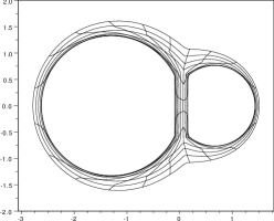
(a) $\delta=0.1$

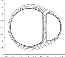
(b) $\delta=0.4$

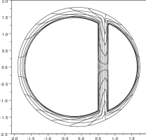
(c) $\delta=0.9$

Figure 4: Transition from round to distorted cavities: $d=1$, $\sqrt{\frac{v_{1}+v_{2}}{\pi d^{2}}}=1.5$, $\frac{v_{2}}{v_{1}}=0.3$.

Our main result (proved in Section 4.1) is the following.

Theorem 2.

Let $\mathbf{a}_{1},\mathbf{a}_{2}\in\mathbb{R}^{n}$, $v_{1}\geq v_{2}\geq 0$, and suppose that $d:=|\mathbf{a}_{1}-\mathbf{a}_{2}|>\varepsilon_{1}+\varepsilon_{2}$. Then, for every $\delta\in[0,1]$ there exists $\mathbf{a^{*}}$ in the line segment joining $\mathbf{a}_{1}$ and $\mathbf{a}_{2}$, and a piecewise smooth map $\mathbf{u}\in C(\mathbb{R}^{n}\setminus\{\mathbf{a}_{1},\mathbf{a}_{2}\},\mathbb{R}^{n})$ satisfying condition INV, such that $\operatorname{Det}D\mathbf{u}=\mathcal{L}^{n}+v_{1}\delta_{\mathbf{a}_{1}}+v_{2}\delta_{\mathbf{a}_{2}}$ in $\mathbb{R}^{n}$ and for all $R>0$

$$\underset{B(\mathbf{a}^{*},R)\setminus(B_{\varepsilon_{1}}(\mathbf{a}_{1})\cup B_{\varepsilon_{2}}(\mathbf{a}_{2}))}{\int}\frac{1}{n}\left|\frac{D\mathbf{u}}{\sqrt{n-1}}\right|^{n}\,\mathrm{d}\mathbf{x}\leq C_{1}(v_{1}+v_{2}+\omega_{n}R^{n})+v_{1}\left(\log\frac{R}{\varepsilon_{1}}\right)_{+}+v_{2}\left(\log\frac{R}{\varepsilon_{2}}\right)_{+}\\ +C_{2}(v_{1}+v_{2})\left((1-\delta)\left(\log\frac{R}{d}\right)_{+}+\delta\left(\sqrt[n]{\frac{v_{2}}{v_{1}}}\log\frac{d}{\varepsilon_{1}}+\sqrt[2n]{\frac{v_{2}}{v_{1}}}\log\frac{d}{\varepsilon_{2}}\right)\right)$$

($C_{1}$ and $C_{2}$ are universal constants depending only on $n$).

If we are not preoccupied with boundary conditions but just wish to build a test configuration with cavities of prescribed volumes and cavitation points at distance $d$, then the above result suffices. This is obtained by our construction of an explicit family of incompressible maps, which contains parameters allowing for all possible cavitation points distances $d$ and cavity volumes $v_{1},v_{2}$. The feature of this construction is that it allows for our almost optimal estimates, as the shapes of the cavities are automatically adjusted to the optimal scenario according to the ratio between $d,\varepsilon,\sqrt{v_{1}},\sqrt{v_{2}}$, their logs, etc, as in the three scenarii of the end of the previous subsection. In other words, the construction builds cavities which, when $d$ is comparable to $\varepsilon$, are distorted and form one equivalent round cavity while the deformation rapidly becomes radially symmetric (as in Scenario (iii)); and cavities which are more and more round as $d$ gets large compared to $\varepsilon$ (as in Scenario (i)). For the extreme cases $\delta=1$ and $\delta=0$, the maps are those that were presented in Figures 2 and 3 respectively. The result for intermediate values of $\delta$ is shown in Figure 4.

Figure 5: Geometric construction of domains $\Omega_{1}$, $\Omega_{2}$ satisfying $\frac{|\Omega_{1}|}{|\Omega_{2}|}=\frac{v_{1}}{v_{2}}$.

The idea of the construction is the following. Take two intersecting balls $B(\mathbf{\tilde{a}}_{1},\rho_{1})$ and $B(\mathbf{\tilde{a}}_{2},\rho_{2})$ such that the width of their union is exactly $2d$ and the width of their intersection is $2d\delta$, and let $\Omega_{1}$ and $\Omega_{2}$ be as in Figure 5 (the precise definition is given in (4.2)). As will be proved in Section 4.1, for every $\delta\in[0,1]$ there are unique $\rho_{1}$ and $\rho_{2}$ such that $\frac{|\Omega_{1}|}{|\Omega_{2}|}=\frac{v_{1}}{v_{2}}$. The cavitation points $\mathbf{a}_{1}$ and $\mathbf{a}_{2}$ are suitably placed in $\Omega_{1}$ and $\Omega_{2}$, respectively, in such a way that $|\mathbf{a}_{1}-\mathbf{a}_{2}|=d$. It is always possible to choose $\mathbf{a^{*}}$ between $\mathbf{a}_{1}$ and $\mathbf{a}_{2}$ such that $\overline{\Omega_{1}\cup\Omega_{2}}$ is star-shaped with respect to $\mathbf{a}^{*}$. In order to define $\mathbf{u}$ in $\mathbb{R}^{n}\setminus\overline{\Omega_{1}\cup\Omega_{2}}$ we choose $\mathbf{a}^{*}$ as the origin and look for an angle-preserving map

$$\mathbf{u}(\mathbf{x})=\lambda\mathbf{a}^{*}+f(\mathbf{x})\frac{\mathbf{x}-\mathbf{a}^{*}}{|\mathbf{x}-\mathbf{a}^{*}|},\qquad\lambda^{n}-1:=\frac{v_{1}+v_{2}}{|\Omega_{1}\cup\Omega_{2}|}=\frac{v_{1}}{|\Omega_{1}|}=\frac{v_{2}}{|\Omega_{2}|}.$$

By so doing, we can solve the incompressibility equation $\det D\mathbf{u}=1$ explicitly, since for angle-preserving maps the equation has the same form as in the radial case,

$$\det D\mathbf{u}(\mathbf{x})=\frac{f^{n-1}(\mathbf{x})\frac{\partial f}{\partial r}(\mathbf{x})}{r^{n-1}}\equiv 1,\quad r=|\mathbf{x}-\mathbf{a^{*}}|,$$

which we will see can be solved as

$$f^{n}(\mathbf{x})=|\mathbf{x}-\mathbf{a}^{*}|^{n}+A\left(\frac{\mathbf{x}-\mathbf{a^{*}}}{|\mathbf{x}-\mathbf{a^{*}}|}\right)^{n},$$

where the function $A:\mathbb{S}^{n-1}\to\mathbb{R}$ is completely determined if we prescribe $\mathbf{u}$ on $\partial\Omega_{1}\cup\partial\Omega_{2}$. Inside $\Omega_{1}$ and $\Omega_{2}$ the deformation $\mathbf{u}$ is defined analogously, taking $\mathbf{a}_{1}$ and $\mathbf{a}_{2}$ as the corresponding origins. The resulting map creates cavities at $\mathbf{a}_{1}$ and $\mathbf{a}_{2}$ with the desired volumes, and with exactly the same shape as $\partial\Omega_{1}$ and $\partial\Omega_{2}$. For compatibility we impose $\mathbf{u}(\mathbf{x})=\lambda\mathbf{x}$ on $\partial\Omega_{1}\cup\partial\Omega_{2}$.

In the energy estimate, $(1-\delta)\log\frac{R}{d}$ is the excess energy due to the distortion of the ‘outer’ curves $\mathbf{u}(\partial B(\mathbf{a^{*}},r))$, $r\in(d,R)$, and $\delta\left(\sqrt[n]{\frac{v_{2}}{v_{1}}}\log\frac{d}{\varepsilon_{1}}+\sqrt[2n]{\frac{v_{2}}{v_{1}}}\log\frac{d}{\varepsilon_{2}}\right)$ is that due to the distortion of the curves $\mathbf{u}(\partial B(\mathbf{a_{i}},r))$, $r\in(\varepsilon_{i},d)$, $i=1,2$ near the cavities. When $\delta=0$, $\overline{\Omega_{1}}$ and $\overline{\Omega_{2}}$ are tangent balls, the cavities are spherical, and the second term in the estimate vanishes. The outer curves are distorted because their shape depends on that of $\partial(\Omega_{1}\cup\Omega_{2})$, hence a price of the order of $(v_{1}+v_{2})\log\frac{R}{d}$ is felt in the energy. When $\delta=1$, at the opposite end, $\Omega_{1}\cup\Omega_{2}$ is a ball of radius $d$, the deformation is radially symmetric outside $\Omega_{1}\cup\Omega_{2}$, and no extra price for the outer curves is paid. In contrast, the cavities are “D-shaped” (they are copies of $\partial\Omega_{1}$ and $\partial\Omega_{2}$), and a price of order $(v_{1}+v_{2})\sqrt[2n]{\frac{v_{2}}{v_{1}}}\log\frac{d}{\varepsilon}$ is obtained as a consequence (in this case the excess energy vanishes as $\frac{v_{2}}{v_{1}}\to 0$, in agreement with the prediction of Theorem 1).

Since the last term of the energy estimate is linear in $\delta$, by taking either $\delta=0$ or $\delta=1$ (and assuming $R>d$) the estimate becomes

$$C(v_{1}+v_{2})\min\left\{\log\frac{R}{d},\sqrt[n]{\frac{v_{2}}{v_{1}}}\log\frac{d}{\varepsilon_{1}}+\sqrt[2n]{\frac{v_{2}}{v_{1}}}\log\frac{d}{\varepsilon_{2}}\right\}.$$

Comparing it against the corresponding term for the lower bound, namely,

$$C(v_{1}+v_{2})\min\left\{\left(\frac{v_{2}}{v_{1}}\right)^{\frac{n}{n-1}}\log\frac{R}{d},\left(\frac{v_{2}}{v_{1}}\right)^{\frac{n}{n-1}}\log\frac{d}{\max\{\varepsilon_{1},\varepsilon_{2}\}}\right\},$$

we observe that there are still some qualitative differences. First of all, in the case when $\varepsilon_{1}\ll\varepsilon_{2}$, a term of the form $\log\frac{d}{\varepsilon_{1}}+\log\frac{d}{\varepsilon_{2}}$ is much larger than $\log\frac{d}{\max\{\varepsilon_{1},\varepsilon_{2}\}}$. We believe that the expression in the lower bound quantifies more accurately the effect of the distortion of the cavities, and that the obstacle for obtaining a comparable expression in the upper bound is that the domains $\Omega_{1}$ and $\Omega_{2}$ in our explicit constructions are required to be star-shaped. For example, in the case $d\sim\varepsilon_{2}$, an energy minimizing deformation $\mathbf{u}$ would try to create a spherical cavity at $\mathbf{a}_{1}$ (so as to prevent a term of order $\log\frac{d}{\varepsilon_{1}}$ from appearing in the energy due to the distortion of the first cavity), and, at the same time, to rapidly become radially symmetric (because of the price of order $\log\frac{R}{d}$ due to the distortion of the ‘outer’ circles). Therefore, for values of $\pi\varepsilon_{2}^{2}\ll v_{1}+v_{2}$, the second cavity would be of the form $B\setminus B_{1}$ for some balls $B_{1}$ and $B$ such that $B_{1}\subset B$, $|B_{1}|=v_{1}$, and $|B|=v_{1}+v_{2}$. In other words, $\mathbf{u}$ must create “moon-shaped” cavities, which cannot be obtained if $\mathbf{u}$ is angle-preserving.

In the second place, the interaction term in the lower bound vanishes as $\frac{v_{2}}{v_{1}}\to 0$ regardless of whether the minimum is achieved at $\log\frac{R}{d}$ or at $\log\frac{d}{\varepsilon}$, whereas in the upper bound this vanishing effect is obtained only for the case of distorted cavities (when $\log\frac{d}{\varepsilon}$ is the smallest). This is because when $\delta=0$ and $v_{1}\gg v_{2}$, the circular sector $\{\mathbf{a}^{*}+de^{i\theta},\theta\in(\frac{\pi}{2},\frac{3\pi}{2})\}$ is mapped to a curve $\lambda\mathbf{a}^{*}+f(\varphi)e^{i\varphi}$ with polar angles $\varphi$ ranging almost from $0$ to $2\pi$. This “angular distortion” necessarily produces a strict inequality in (1.9), so in principle it could be possible to quantify its effect in the lower bound. It is not clear, however, whether for a minimizer an interaction term of the form $(v_{1}+v_{2})\log\frac{R}{d}$ will always be present (in the case when $\frac{v_{2}}{v_{1}}\to 0$), or if the fact that such a term appears in the upper bound is a limitation of the method used for the explicit constructions.

Finally, the factor $\frac{v_{2}}{v_{1}}$ in front of $\log\frac{d}{\varepsilon_{1}}$ and $\log\frac{d}{\varepsilon_{2}}$ is raised to a different exponent in each term, the reason being that $\Omega_{1}$ and $\Omega_{2}$ play different roles in the upper bound construction. Provided $\delta>0$, when $\frac{v_{2}}{v_{1}}\to 0$ the first subdomain is becoming more and more like a circle (its height and its width tend to be equal, and the distortion of the first cavity tends to vanish) whereas $\Omega_{2}$ becomes increasingly distorted (the ratio between its height and its width tends to infinity). The factor $\sqrt[2n]{\frac{v_{2}}{v_{1}}}$ in front of $\log\frac{d}{\varepsilon_{2}}$ is only due to the fact that the effect in the energy of the distortion of the cavities also depends on the size of the cavity.

Dirichlet boundary conditions

If we want our maps to satisfy specific Dirichlet boundary conditions, then they need to be “completed” outside of the ball $B(\mathbf{a^{*}},R)$ of the previous theorem. For that we use the method of Rivière and Ye, and show how to obtain explicit Dirichlet energy estimates from it. We consider the radially symmetric loading of a ball, but other boundary conditions could also be handled. Let $\mathbf{a^{*}}$, $\delta$, $\rho_{1}$, $\rho_{2}$, $\Omega_{1}$, $\Omega_{2}$ be as before. We are to find $R_{1}$, $R_{2}$, and an incompressible diffeomorphism $\mathbf{u}:\{R_{1}<|\mathbf{x}-\mathbf{a^{*}}|<R_{2}\}\to\mathbb{R}^{n}$ such that

1. $\Omega_{1}\cup\Omega_{2}\subset B(\mathbf{a^{*}},R_{1})$ and $\mathbf{u}|_{\partial B(\mathbf{a^{*}},R_{1})}$ coincides with the map of Theorem 2

2. $\mathbf{u}|_{\partial B(\mathbf{a}^{*},R_{2})}$ is radially symmetric.

(a) $\delta=0.1$, reference configuration,
$\pi(R_{2}^{2}-R_{1}^{2})=3.06(v_{1}+v_{2})(1-\delta)$

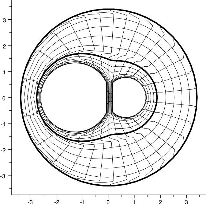
(d) $\delta=0.1$, deformed configuration.
Thick line at $\mathbf{u}(\partial B(\mathbf{a}^{*},R_{1}))$.

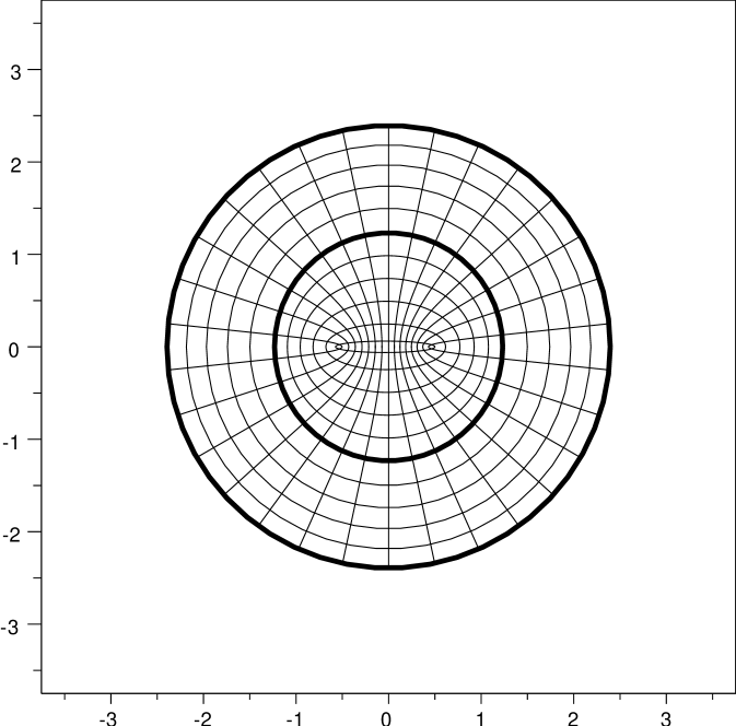
(b) $\delta=0.4$, reference configuration,
$\pi(R_{2}^{2}-R_{1}^{2})=3.12(v_{1}+v_{2})(1-\delta)$

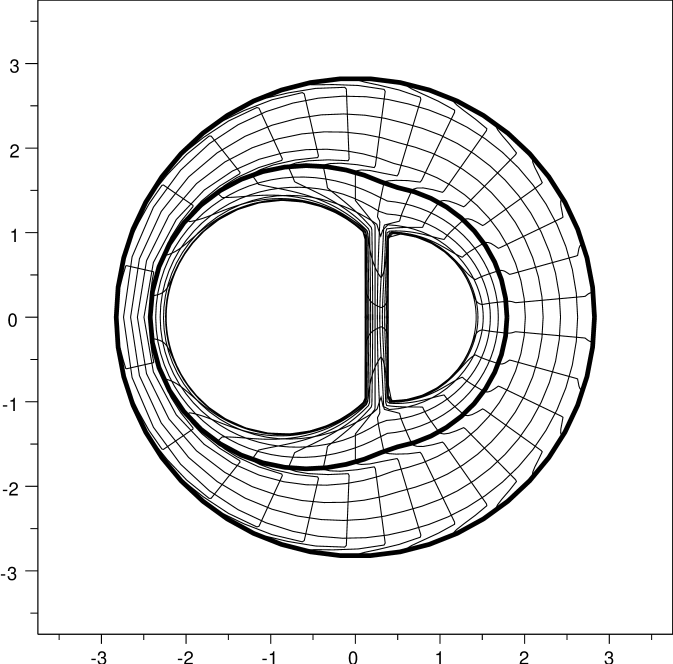
(e) $\delta=0.4$, deformed configuration.
Thick line at $\mathbf{u}(\partial B(\mathbf{a}^{*},R_{1}))$

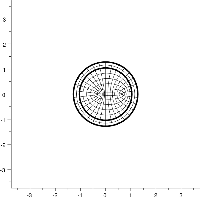
(c) $\delta=0.9$, reference configuration,
$\pi(R_{2}^{2}-R_{1}^{2})=2.46(v_{1}+v_{2})(1-\delta)$

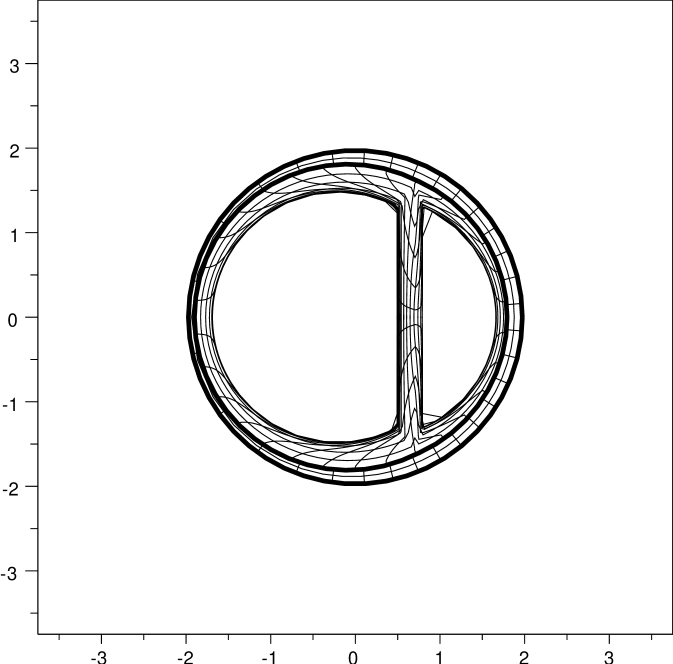
(f) $\delta=0.9$, deformed configuration.
Thick line at $\mathbf{u}(\partial B(\mathbf{a}^{*},R_{1}))$

Figure 6: Transition to a radially symmetric map. A larger initial domain is necessary in order to create spherical cavities. Parameters: $\Omega=B(\mathbf{0},R_{2})$, $\sqrt{\frac{v_{1}+v_{2}}{\pi d^{2}}}=1.5$, $\frac{v_{2}}{v_{1}}=0.3$, $d=1$, $R_{1}\approx d$.

Not all values of $R_{1}$ and $R_{2}$ are suitable for the existence of a solution, since the reference configuration $\{R_{1}\leq|\mathbf{x}-\mathbf{a^{*}}|\leq R_{2}\}$ must contain enough material to fill the space between $\mathbf{u}(\partial B(\mathbf{a^{*}},R_{2}))$ (with shape prescribed by the Dirichlet data) and $\mathbf{u}(\partial B(\mathbf{\mathbf{a}^{*}},R_{1}))$ (whose shape is determined by Theorem 2, see Figure 6). In the case of a radially symmetric loading, the farther $\Omega_{1}\cup\Omega_{2}$ is from being a ball, the larger the reference configuration has to be. If $\delta=1$ nothing has to be imposed; if $\delta<1$, we must have that

$$\omega_{n}(R_{2}^{n}-R_{1}^{n})\geq C(v_{1}+v_{2})(1-\delta)$$

for some constant $C$ (see Lemma 4.5). It turns out that the above necessary condition is also sufficient, as we show in the following theorem:

Theorem 3.

Suppose that $\mathbf{a}_{1}$, $\mathbf{a}_{2}\in\mathbb{R}^{n}$ and $d:=|\mathbf{a}_{1}-\mathbf{a}_{2}|>\varepsilon_{1}+\varepsilon_{2}$. Let $\delta\in[0,1]$, $v_{1}\geq v_{2}\geq 0$,

$$V_{\delta}:=2^{2n+1}n(v_{1}+v_{2})(1-\delta),\qquad R_{1}\geq\max\left\{\sqrt[n]{\frac{V_{\delta}}{\omega_{n}}},2d\right\},\qquad R_{2}:=\sqrt[n]{R_{1}^{n}+\frac{V_{\delta}}{\omega_{n}}}.$$ (1.15)

Then there exists $\mathbf{a^{*}}$ in the segment joining $\mathbf{a}_{1}$ and $\mathbf{a}_{2}$ and a piecewise smooth homeomorphism $\mathbf{u}\in W^{1,\infty}(\mathbb{R}^{n}\setminus\{\mathbf{a}_{1},\mathbf{a}_{2}\},\mathbb{R}^{n})$ such that $\operatorname{Det}D\mathbf{u}=\mathcal{L}^{n}+v_{1}\delta_{\mathbf{a}_{1}}+v_{2}\delta_{\mathbf{a}_{2}}$ in $\mathbb{R}^{n}$, $\mathbf{u}|_{\mathbb{R}^{n}\setminus B(\mathbf{a^{*}},R_{2})}$ is radially symmetric, and for all $R\geq R_{1}$

$$\frac{1}{n}\int_{B(\mathbf{a}^{*},R)\setminus(B_{\varepsilon_{1}}(\mathbf{a}_{1})\cup B_{\varepsilon_{2}}(\mathbf{a}_{2}))}\left|\frac{D\mathbf{u}}{\sqrt{n-1}}\right|^{n}\,\mathrm{d}\mathbf{x}\leq C_{1}(v_{1}+v_{2}+\omega_{n}R^{n})+v_{1}\log\frac{R}{\varepsilon_{1}}+v_{2}\log\frac{R}{\varepsilon_{2}}\\ +C_{2}(v_{1}+v_{2})\left((1-\delta)\left(\log\sqrt[n]{\frac{V_{\delta}}{\omega_{n}d^{n}}}\right)_{+}+\delta\left(\sqrt[n]{\frac{v_{2}}{v_{1}}}\log\frac{d}{\varepsilon_{1}}+\sqrt[2n]{\frac{v_{2}}{v_{1}}}\log\frac{d}{\varepsilon_{2}}\right)\right).$$

The main differences with respect to Theorem 2 are that $\mathbf{u}$ is now radially symmetric in $\mathbb{R}^{n}\setminus B(\mathbf{a}^{*},R_{2})$ and that $\log\frac{R}{d}$ has been replaced with $\log\sqrt[n]{\frac{V_{\delta}}{\omega_{n}d^{n}}}=C+\log\sqrt[n]{\frac{(v_{1}+v_{2})(1-\delta)}{\omega_{n}d^{n}}}$ in the interaction term. The proof is presented in Section 4.2. As a consequence we finally obtain

Corollary 1.

Let $\Omega$ be a ball of radius $R\geq 2d$, with $d>\varepsilon_{1}+\varepsilon_{2}>0$. Then, for every $v_{1}\geq v_{2}\geq 0$ there exist $\mathbf{a}_{1}$, $\mathbf{a}_{2}\in\Omega$ with $|\mathbf{a}_{1}-\mathbf{a}_{2}|=d$, and a Lipschitz homeomorphism $\mathbf{u}:\Omega\setminus\{\mathbf{a}_{1},\mathbf{a}_{2}\}\to\mathbb{R}^{n}$, such that $\operatorname{Det}D\mathbf{u}=\mathcal{L}^{n}+v_{1}\delta_{\mathbf{a}_{1}}+v_{2}\delta_{\mathbf{a}_{2}}$ in $\Omega$, $\mathbf{u}|_{\partial\Omega}\equiv\lambda\mathbf{id}$ (with $\lambda^{n}-1:=\frac{v_{1}+v_{2}}{|\Omega|}$), and

$$\frac{1}{n}\int_{\Omega\setminus(B_{\varepsilon_{1}}(\mathbf{a}_{1})\cup B_{\varepsilon_{2}}(\mathbf{a}_{2}))}\left|\frac{D\mathbf{u}}{\sqrt{n-1}}\right|^{n}\,\mathrm{d}\mathbf{x}\leq C_{1}(v_{1}+v_{2}+\omega_{n}R^{n})+v_{1}\log\frac{R}{\varepsilon_{1}}+v_{2}\log\frac{R}{\varepsilon_{2}}\\ +C_{2}(v_{1}+v_{2})\min_{\delta\in[\delta_{0},1]}\left((1-\delta)\left(\log\frac{(v_{1}+v_{2})(1-\delta)}{\omega_{n}d^{n}}\right)_{+}+\delta\left(\sqrt[n]{\frac{v_{2}}{v_{1}}}\log\frac{d}{\varepsilon_{1}}+\sqrt[2n]{\frac{v_{2}}{v_{1}}}\log\frac{d}{\varepsilon_{2}}\right)\right)$$

with $\delta_{0}:=\max\left\{0,1-\frac{|\Omega|-2^{n}\omega_{n}d^{n}}{4^{n+1}n\omega_{n}d^{n}}\right\}$.

The value of $\delta_{0}$ is such that $\delta\geq\delta_{0}$ if and only if $\omega_{n}R^{n}\geq\omega_{n}R_{1}^{n}+V_{\delta}$, with $\omega_{n}R_{1}^{n}:=V_{\delta}+\omega_{n}(2d)^{n}$; the idea is to be able to use Theorem 3 and obtain a final energy estimate depending only on $v_{1}$, $v_{2}$, $d$, $\varepsilon_{1}$, $\varepsilon_{2}$ and the size $|\Omega|$ of the domain.

1.4 Convergence results

Once we have upper and lower bounds, we are able to show that for “almost-minimizers” one of the three scenarii described after Theorem 1 holds in the limit $\varepsilon\to 0$.

Theorem 4.

Let $\Omega$ be an open and bounded set in $\mathbb{R}^{n}$, $n\geq 2$. Let $\varepsilon_{j}\to 0$ be a sequence, that we will denote in the sequel simply by $\varepsilon$. Let $\{\Omega_{\varepsilon}\}_{\varepsilon}$ be a corresponding sequence of domains of the form $\Omega_{\varepsilon}=\Omega\setminus\bigcup_{i=1}^{m}\overline{B}_{\varepsilon}(\mathbf{a}_{1,\varepsilon})$, with $m\in\mathbb{N}$, $\mathbf{a}_{1,\varepsilon},\ldots,\mathbf{a}_{m,\varepsilon}\in\Omega$ and $\varepsilon$ such that the balls $B_{\varepsilon}(\mathbf{a}_{1,\varepsilon}),\ldots,B_{\varepsilon}(\mathbf{a}_{m,\varepsilon})$ are disjoint. Assume that for each $i=1,\ldots,m$ the sequence $\{\mathbf{a}_{i,\varepsilon}\}_{\varepsilon}$ is compactly contained in $\Omega$. Suppose, further, that there exists $\mathbf{u}_{\varepsilon}\in W^{1,n}(\Omega_{\varepsilon},\mathbb{R}^{n})$ satisfying condition INV, $\operatorname{Det}D\mathbf{u}_{\varepsilon}=\mathcal{L}^{n}$ in $\Omega_{\varepsilon}$, $\sup_{\varepsilon}\|\mathbf{u}_{\varepsilon}\|_{L^{\infty}(\Omega_{\varepsilon})}<\infty$ and

$$\frac{1}{n}\int_{\Omega_{\varepsilon}} \left|\frac{D\mathbf{u}_{\varepsilon}(\mathbf{x})}{\sqrt{n-1}}\right|^{n}\,\mathrm{d}\mathbf{x}\leq\left(\sum_{i=1}^{m}v_{i,\varepsilon}\right)\log\frac{\operatorname{diam}\Omega}{\varepsilon}+C\left(|\Omega|+\sum_{i=1}^{m}v_{i,\varepsilon}\right),$$ (1.16)

where $v_{i,\varepsilon}:=|E(\mathbf{a}_{i,\varepsilon},\varepsilon;\mathbf{u}_{\varepsilon})|-\omega_{n}\varepsilon^{n}$ and $C$ is a universal constant.

Then (extracting a subsequence) the limits $\mathbf{a}_{i}=\lim_{\varepsilon\to 0}\mathbf{a}_{i,\varepsilon}$ and $v_{i}=\lim_{\varepsilon\to 0}{v_{i,\varepsilon}}$, $i=1,\ldots,m$ are well defined, and there exists $\mathbf{u}\in\cap_{1\leq p<n}W^{1,p}(\Omega,\mathbb{R}^{n})\cap W^{1,n}_{\operatorname{loc}}\big{(}\Omega\setminus\{\mathbf{a}_{1},\ldots,\mathbf{a}_{m}\},\mathbb{R}^{n}\big{)}$ such that

• $\mathbf{u}_{\varepsilon}\rightharpoonup\mathbf{u}$ in $W^{1,n}_{\operatorname{loc}}\big{(}\Omega\setminus\{\mathbf{a}_{1},\ldots,\mathbf{a}_{m}\},\mathbb{R}^{n}\big{)}$

• $\operatorname{Det}D\mathbf{u}_{\varepsilon}\overset{*}{\rightharpoonup}\operatorname{Det}D\mathbf{u}$ in $\Omega\setminus\{\mathbf{a}_{1},\ldots,\mathbf{a}_{m}\}$ locally in the sense of measures

• $\operatorname{Det}D\mathbf{u}=\sum_{i=1}^{m}v_{i}\delta_{\mathbf{a}_{i}}+\mathcal{L}^{n}$ in $\Omega$.

When $m=2$, one of the following holds:

1. if $\mathbf{a}_{1}\neq\mathbf{a}_{2}$ and $v_{1},v_{2}>0$ (assume without l.o.g. $v_{1}\geq v_{2}$), then

   • the cavities $\operatorname{im_{T}}(\mathbf{u},\mathbf{a}_{1})$ and $\operatorname{im_{T}}(\mathbf{u},\mathbf{a}_{2})$ (as defined in (2.3)) are balls of volume $v_{1}$, $v_{2}$

   • $|E(\mathbf{a}_{i,\varepsilon},\varepsilon;\mathbf{u}_{\varepsilon})\triangle\operatorname{im_{T}}(\mathbf{u},\mathbf{a}_{i})|\to 0$ as $\varepsilon\to 0$ for $i=1,2$

   • under the additional assumption that $v_{1}+v_{2}<2^{n}\omega_{n}(\operatorname{dist}(\frac{\mathbf{a}_{1}+\mathbf{a}_{2}}{2},\partial\Omega))^{n}$,

     $$\frac{\omega_{n}|\mathbf{a}_{2}-\mathbf{a}_{1}|^{n}}{v_{1}+v_{2}}\geq C_{1}\exp\left(-C_{2}\left(1+\frac{|\Omega|}{v_{1}+v_{2}}+\log\frac{\omega_{n}(\operatorname{diam}\Omega)^{n}}{v_{1}+v_{2}}\right)\left/\left(\frac{v_{2}}{v_{1}+v_{2}}\right)^{\frac{n}{n-1}}\right.\right)$$

     for some positive constants $C_{1}$ and $C_{2}$ depending only on $n$;

2. if $\min\{v_{1},v_{2}\}=0$ (say $v_{2}=0$), then $im_{T}(\mathbf{u},\mathbf{a}_{1})$ (the only cavity opened by $\mathbf{u}$) is spherical;

3. if $\mathbf{a}_{1}=\mathbf{a}_{2}$ and $v_{1},v_{2}>0$ (assume $v_{1}\geq v_{2}$), then

   • $\operatorname{im_{T}}(\mathbf{u},\mathbf{a}_{1})$ is a ball of volume $v_{1}+v_{2}$

   • $|\mathbf{a}_{2,\varepsilon}-\mathbf{a}_{1,\varepsilon}|=O(\varepsilon)$ as $\varepsilon\to 0$

   • the cavities must be distorted in the following sense ($C_{n}$ being as in Proposition 1.2):

     $$\liminf_{\varepsilon\to 0}\frac{v_{1}D\big{(}E(\mathbf{a}_{1,\varepsilon},\varepsilon;\mathbf{u}_{\varepsilon})\big{)}^{\frac{n}{n-1}}+v_{2}D\big{(}E(\mathbf{a}_{2,\varepsilon},\varepsilon;\mathbf{u}_{\varepsilon})\big{)}^{\frac{n}{n-1}}}{v_{1}+v_{2}}>C_{n}\left(\frac{v_{2}}{v_{1}+v_{2}}\right)^{\frac{n}{n-1}}.$$ (1.17)

In the situation of two cavities, the three cases above correspond to the three scenarii of the end of Section 1.2 in the same order.

The main ingredients for the proof are the comparison of the upper bound (1.16) with the lower bounds Proposition 1.1 and Theorem 1, standard compactness arguments, and an argument introduced by Struwe [77] in the context of Ginzburg-Landau which allows to deduce from the energy bounds sufficient compactness of $\mathbf{u}_{\varepsilon}$.

1.5 Additional comments and remarks

We note first that our analysis works provided that the distance of the cavitation points to the boundary does not get small (thus the domain cannot be too thin either). It is an interesting question to better understand what happens when they do get close to the boundary, as well as the effect of the boundary conditions.

Second, it follows from our work that it is always necessary to compare quantities in the reference configuration with quantities in the deformed configuration, due to the scale-invariance in elasticity. For example, we have shown that a large price needs to be paid (in terms of elastic energy) in order to open spherical cavities whenever the distance between the cavitation points is small compared to the final size of the cavities ($\omega_{n}d^{n}\ll v_{1}+v_{2}$). If we only know that the cavitation points are becoming closer and closer to each other, from this alone we cannot conclude that the cavities will interact and that the total elastic energy will go to infinity, as the following argument shows. Suppose that $\mathbf{u}$ is an incompressible map defined on the unit cube $Q\subset\mathbb{R}^{n}$, opening a cavity, and satisfying affine boundary conditions of the form $\mathbf{u}(\mathbf{x})\equiv\mathbf{A}\mathbf{x}$ on $\partial Q$, $\mathbf{A}\in\mathbb{R}^{n\times n}$. Then, by rescaling $\mathbf{u}$ and reproducing it periodically, it is possible to construct a sequence of incompressible maps creating an increasingly large number of cavities, at cavitation points that are closer and closer to each other, in such a way that all the deformations in the sequence have exactly the same elastic energy (cf. Ball & Murat [7]; see also [60, 49, 50]). This is possible because the cavities themselves are also becoming increasingly smaller, with radii decaying at the same rate as the distance between neighbouring cavitation points. This example also shows that the strategy of filling the material with an arbitrarily large number of small cavities is, in a sense, equivalent to forming a single big cavity (there is no interaction between the singularities). Here we complement that result by showing that if it is not possible to create an infinite number of cavities, then the interaction effects in the energy do become noticeable, and under some circumstances can even be quantified.

Third, we mention that the idea of partitioning the domain and using angle-preserving maps inside the resulting subdomains (as described in Section 1.3) can be used to produce test maps that are incompressible and open any prescribed number of cavities (for example by dividing the initial domain in angular sectors).

Finally, we discuss the case $p\neq n$. It is not clear how to extend the analysis to this case, the main reason being that the energy is no longer conformally invariant while the “ball-construction method” is only suited for such cases. To see this in a simple way, let us consider the case of two cavities, assuming incompressibility, letting $\varepsilon_{1}=\varepsilon_{2}\to 0$, and let us try to reproduce the steps (1.8) and (1.11) with (1.14). The $p$-equivalent of (1.14) obtained by Hölder’s inequality (and by relating $|D\mathbf{u}|^{n-1}$ to the area element $|(\operatorname{cof}D\mathbf{u})\boldsymbol{\nu}|$, see Lemma 3.1) is

$$\int_{\partial B(\mathbf{a},r)}\left|\frac{D\mathbf{u}(\mathbf{x})}{\sqrt{n-1}}\right|^{p}\,\mathrm{d}\mathcal{H}^{n-1}(\mathbf{x})\geq\frac{\operatorname{Per}(E(\mathbf{a},r))^{\frac{p}{n-1}}}{(n\omega_{n}r^{n-1})^{\frac{p}{n-1}-1}}\geq n\omega_{n}^{\frac{n-p}{n}}\frac{|E(\mathbf{a},r)|^{\frac{p}{n}}}{r^{1-(n-p)}}\left(1+CD(E(\mathbf{a},r))^{\frac{p}{n-1}}\right).$$

According to this, when $p\neq n$ we may bound from below the energy in $B(\mathbf{a}_{1},\frac{d}{2})\cup B(\mathbf{a}_{2},\frac{d}{2})$ (with $d=|\mathbf{a}_{2}-\mathbf{a}_{1}|$) by

$$\underset{B(\mathbf{a}_{1},\frac{d}{2})\cup B(\mathbf{a}_{2},\frac{d}{2})}{\int}\frac{\omega_{n}^{\frac{p-n}{n}}}{n}\left|\frac{D\mathbf{u}(\mathbf{x})}{\sqrt{n-1}}\right|^{p}\geq\left(v_{1}^{\frac{p}{n}}+v_{2}^{\frac{p}{n}}\right)\left(\frac{d}{2}\right)^{n-p}+C(v_{1}+v_{2})^{\frac{p}{n}}\int_{0}^{\frac{d}{2}}\langle D(E(\mathbf{a}_{i},r))^{\frac{p}{n-1}}\rangle r^{n-p-1},$$

where $\langle D(E(\mathbf{a}_{i},r)))^{\frac{p}{n-1}}\rangle$ stands for the average distortion

$$\langle D(E(\mathbf{a}_{i},r)))^{\frac{p}{n-1}}\rangle:=\left(v_{1}^{\frac{p}{n}}D(E(\mathbf{a}_{1},r))^{\frac{p}{n-1}}+v_{2}^{\frac{p}{n}}D(E(\mathbf{a}_{2},r))^{\frac{p}{n-1}}\right)(v_{1}+v_{2})^{-\frac{p}{n}}.$$

Analogously, we can bound the energy in $B(\mathbf{a},R)\setminus\overline{B}(\mathbf{a},d)$ (with $\mathbf{a}=\frac{\mathbf{a}_{1}+\mathbf{a}_{2}}{2}$) by

$$\underset{B(\mathbf{a},R)\setminus\overline{B}(\mathbf{a},d)}{\int}\frac{\omega_{n}^{\frac{p-n}{n}}}{n}\left|\frac{D\mathbf{u}(\mathbf{x})}{\sqrt{n-1}}\right|^{p}\geq(v_{1}+v_{2})^{\frac{p}{n}}\int_{d}^{R}r^{n-p-1}+C(v_{1}+v_{2})^{\frac{p}{n}}\int_{d}^{R}D(E(\mathbf{a},r))^{\frac{p}{n-1}}r^{n-p-1}$$

and obtain:

$$\int_{B(\mathbf{a},R)}\frac{\omega_{n}^{\frac{p-n}{n}}}{n}\left|\frac{D\mathbf{u}(\mathbf{x})}{\sqrt{n-1}}\right|^{p}\geq(v_{1}+v_{2})^{\frac{p}{n}}\left(\int_{0}^{\frac{d}{2}}+\int_{d}^{R}\right)r^{n-p-1}+\underbrace{\left(v_{1}^{\frac{p}{n}}+v_{2}^{\frac{p}{n}}-(v_{1}+v_{2})^{\frac{p}{n}}\right)\left(\frac{d}{2}\right)^{n-p}}_{II}\\ +\underbrace{C(v_{1}+v_{2})^{\frac{p}{n}}\left[\int_{0}^{\frac{d}{2}}\langle D(E(\mathbf{a}_{i},r))^{\frac{p}{n-1}}\rangle r^{n-p-1}+\int_{d}^{R}D(E(\mathbf{a},r))^{\frac{p}{n-1}}r^{n-p-1}\right]}_{III}.$$

Assume that $v_{1}+v_{2}$ is fixed (as is the case in the Dirichlet problem). Let us first consider the case $p<n$. Since the limit $\varepsilon\to 0$ is not singular in this case (contrarily to $p=n$), the problem cannot be analyzed by asymptotic analysis. If we guide ourselves only by the second and third terms (II and III), when $p<n$ we can say the following. The factor $v_{1}^{\frac{p}{n}}+v_{2}^{\frac{p}{n}}-(v_{1}+v_{2})^{\frac{p}{n}}$ in II is minimized when $\min\{v_{1},v_{2}\}=0$, hence it motivates the creation of just one cavity (the same can be said for the problem with $M$ cavities, because $v_{1}^{\frac{p}{n}}+\cdots+v_{M}^{\frac{p}{n}}$ is concave and the restriction $v_{1}+\ldots+v_{M}=\text{const.}$ is linear). If the above difference has to be positive, the factor $\left(\frac{d}{2}\right)^{n}$ suggests that the two cavitation points would want to be arbitrarily close, and that the cavities will tend to act as a single cavity. This is consistent with the prediction for III; indeed, consider the corresponding estimate for $p=n$:

$$\frac{1}{n}\int_{\Omega_{\varepsilon}\cap B(\mathbf{a},R)}\left|\frac{D\mathbf{u}(\mathbf{x})}{\sqrt{n-1}}\right|^{n}\,\mathrm{d}\mathbf{x}\geq(v_{1}+v_{2})\left(\int_{\varepsilon}^{\frac{d}{2}}+\int_{d}^{R}\right)\frac{\,\mathrm{d}r}{r}\\ +C(v_{1}+v_{2})\left[\int_{\varepsilon}^{\frac{d}{2}}\langle D(E(\mathbf{a}_{i},r))^{\frac{n}{n-1}}\rangle\frac{\,\mathrm{d}r}{r}+\int_{d}^{R}D(E(\mathbf{a},r))^{\frac{p}{n-1}}\frac{\,\mathrm{d}r}{r}\right].$$

Under a logarithmic cost, it is much more important to minimize the distortions $D(E(\mathbf{a}_{i},r))$ of the circles $\mathbf{u}(\partial B(\mathbf{a}_{i},r))$, $i=1,2$, $\varepsilon<r<\frac{d}{2}$ near the cavities, rather than the distortion of the outer circles $D(E(\mathbf{a},r))$, $r>d$. As was discussed before, this leads either to the case of well-separated and spherical cavities (scenario (i) in p. Scenario (i)), or to the conclusion that if outer circles are mapped to circles (scenario (iii)) then the distance between cavitation points must be of order $\varepsilon$ (Theorem 4iii)). In contrast, When $p<n$, in the presence of the weight $r^{n-p-1}$, minimizing the distortions $D(E(\mathbf{a},r))$, $r>d$ gains more relevance compared to the distortion near the cavities.

For the previous reasons, we believe that the deformations of scenario (i) will not be global minimizers, instead the body will prefer to open a single cavity. If multiple cavities have to be created, then the cavitation points will try to be close to each other, and the deformation will try to rapidly become radially symmetric. The cavities will be distorted and try to act as a single cavity (as in scenario (iii), which creates a state of strain potentially leading to fracture by coalescence), at distances between the cavitation points that are of order $1$ (not of order $\varepsilon$). This, in fact, is what has been observed numerically [81, 47].

Let us now turn to $p>n$. The lower bound reads

$$\int_{\Omega_{\varepsilon}\cap B(\mathbf{a},R)}\frac{\omega_{n}^{\frac{p-n}{n}}}{n}\left|\frac{D\mathbf{u}(\mathbf{x})}{\sqrt{n-1}}\right|^{p}\,\mathrm{d}\mathbf{x}+\frac{(v_{1}+v_{2})^{\frac{p}{n}}}{p-n}R^{n-p}\geq\underbrace{(v_{1}^{\frac{p}{n}}+v_{2}^{\frac{p}{n}})\int_{\varepsilon}^{\frac{d}{2}}r^{n-p-1}}_{I}+\underbrace{(v_{1}+v_{2})^{\frac{p}{n}}d^{n-p}}_{II}\\ +C(v_{1}+v_{2})^{\frac{p}{n}}\left[\int_{\varepsilon}^{\frac{d}{2}}\langle D(E(\mathbf{a}_{i},r))^{\frac{p}{n-1}}\rangle r^{n-p-1}+\int_{d}^{R}D(E(\mathbf{a},r))^{\frac{p}{n-1}}r^{n-p-1}\right].$$

This time the limit $\varepsilon\to 0$ is singular, even more so than for $p=n$. The factor $v_{1}^{\frac{p}{n}}+v_{2}^{\frac{p}{n}}$ is now minimized when the cavities have equal volumes. Regarding $d$, the first term prefers small distances ($d=2\varepsilon$) while the second prefers $d\to\infty$; since $(v_{1}+v_{2})^{\frac{p}{n}}>v_{1}^{\frac{p}{n}}+v_{2}^{\frac{p}{n}}$, it can be said that II has a stronger influence, hence $d$ large should be preferred. With respect to the third term, it is now much more vital to create spherical cavities (so as to minimize the first of the two integrals) than when $p=n$. This implies that it is scenario (i), rather than (ii) or (iii), which should be observed.

The case $p<n$, therefore, should favour a single cavity and coalescence, $p>n$ should favour many cavities and splitting, and both situations are possible in the borderline case that we have studied: $p=n$.

1.6 Plan of the paper

In Section 2 we describe our notation and recall the notions of perimeter, reduced boundary, topological image, distributional determinant, and the invertibility condition INV. In Section 3 we begin by extending (1.14) to the case of an arbitrary power $p$ and space dimension $n$ (Lemma 3.1). In Section 3.1 we prove the lower bound for an arbitrary number of cavities using the ball construction method (Proposition 1.1). In Section 3.2, we prove the main lower bound (Theorem 1) and postpone the proof of our estimate on the distortions (Proposition 1.2) to Section 3.3. The energy estimates for the angle-preserving ansatz are presented in Section 4.1 and proved in Section 4.3. In Section 4.2 we show how to complete the maps away from the cavitation points so as to fulfil the boundary conditions, and in Section 4.4 we comment briefly on the numerical computations presented in this paper based on the constructive method of Dacorogna & Moser [20]. Finally, the proof of the main compactness result and of the fact that in the limit only one of the three scenarii holds (Theorem 4) is given in Section 5.

1.7 Acknowledgements

We give special thanks to G. Francfort for his interest and his involvement in this project. We also thank J.-F. Babadjian, J. Ball, Y. Brenier, A. Contreras, R. Kohn, R. Lecaros, G. Mingione, C. Mora-Corral, S. Müller, T. Rivière, and N. Rougerie for useful discussions.

2 Notation and preliminaries

2.1 General notation

Let $n$ denote the space dimension. Vector-valued and matrix-valued quantities will be written in bold face. The set of unit vectors in $\mathbb{R}^{n}$ is denoted by $\mathbb{S}^{n-1}$. Given a set $E\subset\mathbb{R}^{n}$, $\lambda\geq 0$ and $\mathbf{h}\in\mathbb{R}^{n}$, we define $\lambda E:=\{\lambda\mathbf{x}:\ \mathbf{x}\in E\}$ and $E+\mathbf{h}:=\{\mathbf{x}+\mathbf{h}:\ \mathbf{x}\in E\}$. The interior and the closure of $E$ are denoted by $\operatorname{Int}E$ and $\overline{E}$, and the symmetric difference of two sets $E_{1}$ and $E_{2}$ by $E_{1}\triangle E_{2}$. If $E_{1}$ is compactly contained in $E_{2}$, we write $E_{1}\subset\!\subset E_{2}$. The notations $B(\mathbf{x},R)$, $B_{R}(\mathbf{x})$ are used for the open ball of radius $R$ centred at $\mathbf{x}$, and $\overline{B}(\mathbf{a},R)$, $\overline{B}_{R}(\mathbf{a})$ for the corresponding closed ball. The distance from a point $\mathbf{x}$ to a set $E$ is denoted by $\operatorname{dist}(\mathbf{x},E)$, the distance between sets by $\operatorname{dist}(E_{1},E_{2})$, and the diameter of a set by $\operatorname{diam}E$.

Given $\mathbf{A}$ an $n\times n$ matrix, $\mathbf{A}^{T}$ will be its transpose, $\det\mathbf{A}$ its determinant, and $\operatorname{cof}\mathbf{A}$ its cofactor matrix (defined by $\mathbf{A}^{T}\operatorname{cof}\mathbf{A}=(\det\mathbf{A})\mathbf{1}$, where $\mathbf{1}$ stands for the $n\times n$ identity matrix). The adjugate matrix of $\mathbf{A}$ is $\operatorname{adj}\mathbf{A}=(\operatorname{cof}\mathbf{A})^{T}$.

The Lebesgue and the $k$-dimensional Hausdorff measure are denoted by $\mathcal{L}^{n}$ and $\mathcal{H}^{k}$, respectively. If $E$ is a measurable set, $\mathcal{L}^{n}(E)$ is also written $|E|$ (as well as $|I|$ for the length of an interval $I$). The measure of the $k$-dimensional unit ball is $\omega_{k}$ (accordingly, $\mathcal{H}^{n-1}(\partial B(\mathbf{x},r))=n\omega_{n}r^{n-1}$). The exterior product of $1\leq k\leq n$ vectors $\mathbf{a}_{1},\ldots,\mathbf{a}_{k}\in\mathbb{R}^{n}$ is denoted by $\mathbf{a}_{1}\wedge\cdots\wedge\mathbf{a}_{k}$ or $\bigwedge_{i=1}^{k}\mathbf{a}_{i}$. It is $k$-linear, antisymmetric, and such that $|\mathbf{a}_{1}\wedge\cdots\wedge\mathbf{a}_{k}|$ is the $k$-dimensional measure of the $k$-prism formed by $\mathbf{a}_{1},\ldots\mathbf{a}_{k}$ (see, e.g., [24, 75, 33, 1]). In particular, $|\mathbf{x}|^{2}=|\mathbf{x}\cdot\mathbf{e}|^{2}+|\mathbf{x}\wedge\mathbf{e}|^{2}$ for all $\mathbf{x}\in\mathbb{R}^{n}$ and $\mathbf{e}\in\mathbb{S}^{n-1}$. With a slight abuse of notation, when $k=n$ the expression $\mathbf{a}_{1}\wedge\cdots\wedge\mathbf{a}_{n}$ is used to denote the determinant (in the standard basis) of the matrix with column vectors $\mathbf{a}_{1},\ldots,\mathbf{a}_{n}\in\mathbb{R}^{n}$.

The characteristic function of a set $E$ is referred to as $\chi_{E}$, and the restriction of $\mathbf{u}$ to $E$ as $\mathbf{u}|_{E}$. The sign function $\operatorname{sgn}:\mathbb{R}\to\{-1,0,1\}$ is given by $\operatorname{sgn}x=x/|x|$ if $x\neq 0$, $\operatorname{sgn}0=0$. The notation $\mathbf{id}$ is used for the identity function $\mathbf{id}(\mathbf{x})\equiv\mathbf{x}$. The symbol $\fint_{E}f$ stands for the integral average $\frac{1}{|E|}{\int_{E}f}$. The support of a function $f$ is represented by $\operatorname{spt}f$.

The space of infinitely differentiable functions with compact support is denoted by $C_{c}^{\infty}(\Omega)$, and the $L^{p}$ norm of a function $f$ by $\|f\|_{L^{p}}$. Sobolev spaces are denoted by $W^{1,p}(\Omega,\mathbb{R}^{n})$, as usual. The Hilbert space $W^{1,2}(\Omega,\mathbb{R}^{n})$ is denoted by $H^{1}(\Omega,\mathbb{R}^{n})$. The weak derivative (the linear transformation) of a map $\mathbf{u}\in W^{1,p}(\Omega,\mathbb{R}^{n})$ at a point $\mathbf{x}\in\mathbb{R}^{n}$ is identified with the gradient $D\mathbf{u}(\mathbf{x})$ (the matrix of weak partial derivatives).

Use will be made of the coarea formula (see, e.g., [24, 23, 1]): if $E\subset\mathbb{R}^{n}$ is measurable and $\phi:E\to\mathbb{R}$ is Lipschitz, then for all $f\in L^{1}(E)$

$$\int_{E}f(\mathbf{x})|D\phi(\mathbf{x})|\,\mathrm{d}\mathbf{x}=\int_{-\infty}^{\infty}\left(\int_{\{\mathbf{x}\in E:\phi(\mathbf{x})=t\}}f(\mathbf{x})\,\mathrm{d}\mathcal{H}^{n-1}(\mathbf{x})\right)\,\mathrm{d}t.$$

2.2 Perimeter and reduced boundary

Definition 2.

The perimeter of a measurable set $E\subset\mathbb{R}^{n}$ is defined as

$$\operatorname{Per}E:=\sup\left\{\int_{E}\operatorname{div}\mathbf{g}(\mathbf{y})\,\mathrm{d}\mathbf{y}:\mathbf{g}\in C^{1}_{c}(\mathbb{R}^{n},\mathbb{R}^{n}),\|\mathbf{g}\|_{\infty}\leq 1\right\}.$$

Definition 3.

Given $\mathbf{y}_{0}\in\mathbb{R}^{n}$ and a non-zero vector $\boldsymbol{\nu}\in\mathbb{R}^{n}$, we define

$$H^{+}(\mathbf{y}_{0},\boldsymbol{\nu}):=\{\mathbf{y}\in\mathbb{R}^{n}:(\mathbf{y}-\mathbf{y}_{0})\cdot\boldsymbol{\nu}\geq 0\},\quad H^{-}(\mathbf{y}_{0},\boldsymbol{\nu}):=\{\mathbf{y}\in\mathbb{R}^{n}:(\mathbf{y}-\mathbf{y}_{0})\cdot\boldsymbol{\nu}\leq 0\}.$$

The reduced boundary of a measurable set $E\subset\mathbb{R}^{n}$, denoted by $\partial^{*}E$, is defined as the set of points $\mathbf{y}\in\mathbb{R}^{n}$ for which there exists a unit vector $\boldsymbol{\nu}\in\mathbb{R}^{n}$ such that

$$\lim_{r\to 0^{+}}\frac{|E\cap H^{-}(\mathbf{y},\boldsymbol{\nu})\cap B(\mathbf{y},r)|}{|B(\mathbf{y},r)|}=\frac{1}{2}\quad\text{and}\quad\lim_{r\to 0^{+}}\frac{|E\cap H^{+}(\mathbf{y},\boldsymbol{\nu})\cap B(\mathbf{y},r)|}{|B(\mathbf{y},r)|}=0.$$

If $\mathbf{y}\in\partial^{*}E$ then $\boldsymbol{\nu}$ is uniquely determined and is called the unit outward normal to $E$.

The definition of perimeter coincides precisely with the $\mathcal{H}^{n-1}$-measure of the reduced boundary, as follows from the well-known results of Federer, Fleming and De Giorgi (see, e.g., [24, 83, 23, 1]).

2.3 Degree and topological image

We begin by recalling the notion of topological degree for maps $\mathbf{u}$ that are only weakly differentiable [56, 26, 12, 17].

If $\mathbf{u}\in W^{1,p}(\Omega,\mathbb{R}^{n})$ and $\mathbf{x}\in\mathbb{R}^{n}$, then, for a.e. $r\in(0,\infty)$ with $\partial B(\mathbf{x},r)\subset\Omega$,

• $\mathbf{u}(\mathbf{z})$ and $D\mathbf{u}(\mathbf{z})$ are defined at $\mathcal{H}^{n-1}$-a.e. $\mathbf{z}\in\partial B(\mathbf{x},r)$

• $\mathbf{u}|_{\partial B(\mathbf{x},r)}\in W^{1,p}(\partial B(\mathbf{x},r),\mathbb{R}^{n})$

• $D(\mathbf{u}|_{\partial B(\mathbf{x},r)})(\mathbf{z})=(D\mathbf{u}(\mathbf{z}))|_{T_{\mathbf{z}}(\partial B(\mathbf{x},r))}$ (the $n$-dimensional and the tangential weak derivatives coincide; $T_{\mathbf{z}}(\partial B(\mathbf{x},r))$ denotes the tangent plane) for $\mathcal{H}^{n-1}$-a.e. $\mathbf{z}\in\partial B(\mathbf{x},r)$

(this follows by approximating by $C^{\infty}$ maps and using the coarea formula). If, moreover, $p>n-1$, then, by Morrey’s inequality, there exists a unique map $\overline{\mathbf{u}}\in C^{0}(\partial B(\mathbf{x},r))$ that coincides with $\mathbf{u}|_{\partial B(\mathbf{x},r)}$ $\mathcal{H}^{n-1}$-a.e. With an abuse of notation we write $\mathbf{u}(\partial B(\mathbf{x},r))$ to denote $\overline{\mathbf{u}}(\partial B(\mathbf{x},r))$.

If $p>n-1$ and (R2) is satisfied, for every $\mathbf{y}\in\mathbb{R}^{n}\setminus\mathbf{u}(\partial B(\mathbf{x},r))$ we define $\deg(\mathbf{u},\partial B(\mathbf{x},r),\mathbf{y})$ as the classical Brouwer degree [68, 26] of $\mathbf{u}|_{\partial B(\mathbf{x},r)}$ with respect to $\mathbf{y}$. The degree $\deg(\mathbf{u},\partial B(\mathbf{x},r),\cdot)$ is the only $L^{1}(\mathbb{R}^{n})$ map [56, 12] such that

$$\int_{\mathbb{R}^{n}}\deg(\mathbf{u},\partial B(\mathbf{x},r),\mathbf{y})\operatorname{div}\mathbf{g}(\mathbf{y})\,\mathrm{d}\mathbf{y}=\int_{\partial B(\mathbf{x},r)}\mathbf{g}(\mathbf{u}(\mathbf{z}))\cdot(\operatorname{cof}D\mathbf{u}(\mathbf{z}))\boldsymbol{\nu}(\mathbf{z})\,\mathrm{d}\mathcal{H}^{n-1}(\mathbf{z})$$ (2.1)

for every $\mathbf{g}\in C^{1}(\mathbb{R}^{n},\mathbb{R}^{n})$, $\boldsymbol{\nu}(\mathbf{z})$ being the outward unit normal to $\partial B(\mathbf{x},r)$.

For a map $\mathbf{u}\in W^{1,p}(\Omega,\mathbb{R}^{n})$ that is invertible, orientation-preserving, and regular except for the creation of a finite number of cavities, $\deg(\mathbf{u},\partial B(\mathbf{x},r),\mathbf{y})$ is equal to $1$, roughly speaking, only at those points $\mathbf{y}$ enclosed by $\mathbf{u}(\partial B(\mathbf{x},r))$. Because of this, the degree is useful for the study of cavitation, since we can detect a cavity by looking at the set of points where the degree is $1$, but which do not belong to the image of $\mathbf{u}$ (they are not part of the deformed body). This gave rise to Šverák’s notion of topological image [79].

Definition 4.

Let $\mathbf{u}\in W^{1,p}(\partial B(\mathbf{x},r),\mathbb{R}^{n})$ for some $\mathbf{x}\in\mathbb{R}^{n}$, $r>0$, and $p>n-1$. Then

$$\operatorname{im_{T}}(\mathbf{u},B(\mathbf{x},r)):=\{\mathbf{y}\in\mathbb{R}^{n}:\ \deg(\mathbf{u},\partial B(\mathbf{x},r),\mathbf{y})\neq 0\}.$$

It was pointed out by Müller-Spector [55, Sect. 11] that Sobolev maps may create cavities in some part of the body, and subsequently fill them with material from somewhere else (even if they are one-to-one a.e. [3]). In order to avoid this pathological behaviour, they defined a stronger invertibility condition, based on the topological image.

Definition 5.

Let $\mathbf{u}\in W^{1,p}(\Omega,\mathbb{R}^{n})$ with $p>n-1$. We say that $\mathbf{u}$ satisfies condition INV if

1. $\mathbf{u}(\mathbf{z})\in\operatorname{im_{T}}(\mathbf{u},B(\mathbf{x},r))$ for a.e. $\mathbf{z}\in B(\mathbf{x},r)\cap\Omega$

2. $\mathbf{u}(\mathbf{z})\in\mathbb{R}^{n}\setminus\operatorname{im_{T}}(\mathbf{u},B(\mathbf{x},r))$ for a.e. $\mathbf{z}\in\Omega\setminus B(\mathbf{x},r)$

for every $\mathbf{x}\in\mathbb{R}^{n}$ and a.e. $r\in(0,\infty)$ such that $\mathbf{u}|_{\partial B(\mathbf{x},r)}\in W^{1,p}(\partial B(\mathbf{x},r),\mathbb{R}^{n})$.

In the following proposition we summarize some of the main virtues of condition INV. We add a sketch of the proof to make it easier for the interested reader to compile the different ideas and conciliate the different notation in [79], [55, Lemmas 2.5, 3.5 and 7.3], [17, Lemmas 3.8 and 3.10], [39, Lemma 2], and [40, Prop. 6 and Lemma 15].

Proposition 2.1.

Let $\mathbf{u}\in W^{1,p}(\Omega,\mathbb{R}^{n})$ with $p>n-1$ satisfy $\det D\mathbf{u}>0$ a.e. and condition INV. Then, for every $\mathbf{x}\in\mathbb{R}^{n}$ there exists a full-$\mathcal{L}^{1}$-measure subset $R_{\mathbf{x}}$ of $\{r\in(0,\infty):\partial B(\mathbf{x},r)\subset\Omega\}$ for which (R1)–(R3), conditions i)-ii) of Definition 5, and the following properties are satisfied:

1. $\deg(\mathbf{u},\partial B(\mathbf{x},r),\mathbf{y})\in\{0,1\}$ for every $\mathbf{y}\in\mathbb{R}^{n}\setminus{\mathbf{u}}(\partial B(\mathbf{x},r))$

2. $\partial^{*}\operatorname{im_{T}}(\mathbf{u},B(\mathbf{x},r))={\mathbf{u}}(\partial B(\mathbf{x},r))$ up to $\mathcal{H}^{n-1}$-null sets

3. $\displaystyle\operatorname{Per}\big{(}\operatorname{im_{T}}(\mathbf{u},B(\mathbf{x},r))\big{)}=\int_{\partial B(\mathbf{x},r)}|(\operatorname{cof}D\mathbf{u}(\mathbf{z}))\boldsymbol{\nu}(\mathbf{z})|\,\mathrm{d}\mathcal{H}^{n-1}(\mathbf{z})$

4. $|\operatorname{im_{T}}(\mathbf{u},B(\mathbf{x},r))|=\displaystyle\frac{1}{n}\int_{\partial B(\mathbf{x},r)}\mathbf{u}(\mathbf{z})\cdot(\operatorname{cof}D\mathbf{u}(\mathbf{z}))\boldsymbol{\nu}(\mathbf{z})\,\mathrm{d}\mathcal{H}^{n-1}(\mathbf{z})$.

Moreover, for every $\mathbf{x},\mathbf{x}^{\prime}\in\mathbb{R}^{n}$ and every $r\in R_{\mathbf{x}}$, $r^{\prime}\in R_{\mathbf{x}^{\prime}}$

1. $\operatorname{im_{T}}(\mathbf{u},B(\mathbf{x},r))\subset\operatorname{im_{T}}(\mathbf{u},B(\mathbf{x}^{\prime},r^{\prime}))$ if $B(\mathbf{x},r)\subset B(\mathbf{x}^{\prime},r^{\prime})$

2. $\operatorname{im_{T}}(\mathbf{u},B(\mathbf{x},r))\cap\operatorname{im_{T}}(\mathbf{u},B(\mathbf{x}^{\prime},r^{\prime}))=\varnothing$ if $B(\mathbf{x},r)\cap B(\mathbf{x}^{\prime},r^{\prime})=\varnothing$.

Proof.

Call $\Omega_{0}$ the set of $\mathbf{x}\in\Omega$ for which there exist $\mathbf{w}\in C^{1}(\mathbb{R}^{n},\mathbb{R}^{n})$ and a compact set $K\subset\Omega$ such that

$$\lim_{r\to 0^{+}}\frac{|K\cap B(\mathbf{x},r)|}{|B(\mathbf{x},r)|}=1,\quad\mathbf{u}|_{K}=\mathbf{w}|_{K},\quad\text{and}\quad D\mathbf{u}|_{K}=D\mathbf{w}|_{K}.$$ (2.2)

Since $\mathbf{u}\in W^{1,p}(\Omega,\mathbb{R}^{n})$, it is possible to find (combining Federer’s approximation of approximately differentiable maps by Lipschitz functions, Rademacher’s theorem, and Whitney’s extension theorem, see, e.g., [23, Cor. 6.6.3.2], [24, Thms. 3.1.8 and 3.1.16], [55, Prop. 2.4], [39, Lemma 1]) an increasing sequence of compact sets $\{K_{j}\}_{j\in\mathbb{N}}$ contained in $\Omega$, and a sequence $\{\mathbf{w}_{j}\}_{j\in\mathbb{N}}$ of maps in $C^{1}(\mathbb{R}^{n},\mathbb{R}^{n})$, such that $\mathbf{u}|_{K_{j}}=\mathbf{w}_{j}|_{K_{j}}$, $\nabla\mathbf{u}_{j}|_{K_{j}}=D\mathbf{w}|_{K_{j}}$, and $|\Omega\setminus K_{j}|<\frac{1}{j}$ for each $j\in\mathbb{N}$. By Lebesgue’s differentiation theorem, $|K_{j}\setminus K_{j}^{\prime}|=0$ where $K_{j}^{\prime}:=\{\mathbf{x}\in K_{j}:\lim_{r\to 0^{+}}(r^{-n}|B(\mathbf{x},r)\setminus K|)=0\}$. Since $\Omega_{0}\supset\bigcup_{j\in\mathbb{N}}K_{j}^{\prime}$, it follows that $|\Omega\setminus\Omega_{0}|=0$.

Define $R_{\mathbf{x}}$ as the subset of $\{r\in(0,\infty):\partial B(\mathbf{x},r)\subset\Omega\}$ for which (R1)–(R3), conditions i)-ii) of Definition 5, and the following properties are satisfied:

• $\mathcal{H}^{n-1}(\partial B(\mathbf{x},r)\setminus\Omega_{0})=0$

• $\det D\mathbf{u}(\mathbf{z})>0$ for $\mathcal{H}^{n-1}$-a.e. $\mathbf{z}\in\partial B(\mathbf{x},r)$.

The fact that $|\{r\in(0,\infty):\partial B(\mathbf{x},r)\subset\Omega\}\setminus R_{\mathbf{x}}|=0$ is a consequence of the coarea formula and of the discussion before Definition 4. For this choice of $R_{\mathbf{x}}$ we have that the properties listed in the proposition are satisfied for all (not only for a.e.) $r\in R_{\mathbf{x}}$. This follows from (2.1), the fact that $\mathbf{u}_{|\Omega_{0}}$ is one to one (by [55, Lemmas 3.4 and 2.5]; only minor modifications are required, see [39, Lemma 2] if necessary), and a careful inspection of the proofs of [55, Lemmas 2.5, 3.5 and 7.3]. ∎

By Proposition 2.1v) the topological image of $B(\mathbf{x},r)$ can be defined for all $\mathbf{x}\in\mathbb{R}^{n}$ and all $r\geq 0$ such that $\{\mathbf{z}:r<|\mathbf{z}|<r+\delta\}\subset\Omega$ for some $\delta>0$ (not only for radii $r\in R_{\mathbf{x}}$). Indeed, since the sequence $\{\operatorname{im_{T}}(\mathbf{u},B(\mathbf{x},r)):r\in R_{\mathbf{x}}\}$ is increasing for every $\mathbf{x}\in\mathbb{R}^{n}$, we may define

$$E(\mathbf{x},r):=\bigcap_{\begin{subarray}{c}r^{\prime}>r\\ r^{\prime}\in R_{\mathbf{x}}\end{subarray}}\operatorname{im_{T}}(\mathbf{u},B(\mathbf{x},r)).$$ (2.3)

Whenever explicit mention of $\mathbf{u}$ is necessary (such as in Theorem 4 where sequences of deformations are considered), we write $E(\mathbf{a},r;\mathbf{u})$. Finally, if a point $\mathbf{a}\in\mathbb{R}^{n}$ is such that $B(\mathbf{a},\delta)\setminus\{\mathbf{a}\}\subset\Omega$ for some $\delta>0$, we define its topological image as $E(\mathbf{a}_{i},0)$, and denote it by $\operatorname{im_{T}}(\mathbf{u},\mathbf{a})$.

2.4 The distributional determinant

It is well known that the Jacobian determinant of a $C^{2}$ vector-valued map $\mathbf{u}:\Omega\subset\mathbb{R}^{n}\to\mathbb{R}^{n}$ has a divergence structure. When $n=2$ or $n=3$, this is

$$\det D\mathbf{u} =u_{1,1}u_{2,2}-u_{2,1}u_{1,2}=(u_{1}u_{2,2})_{,1}-(u_{1}u_{2,1})_{,2}$$

$$\det D\mathbf{u} =u_{1,1}\left|\begin{array}[]{cc}u_{2,2}&u_{2,3}\\ u_{3,2}&u_{3,3}\end{array}\right|+u_{1,2}\left|\begin{array}[]{cc}u_{2,3}&u_{2,1}\\ u_{3,3}&u_{3,1}\end{array}\right|+u_{1,3}\left|\begin{array}[]{cc}u_{2,1}&u_{2,2}\\ u_{3,1}&u_{3,2}\end{array}\right|$$

$$=\left(u_{1}\left|\begin{array}[]{cc}u_{2,2}&u_{2,3}\\ u_{3,2}&u_{3,3}\end{array}\right|\right)_{,1}+\left(u_{1}\left|\begin{array}[]{cc}u_{2,3}&u_{2,1}\\ u_{3,3}&u_{3,1}\end{array}\right|\right)_{,2}+\left(u_{1}\left|\begin{array}[]{cc}u_{2,1}&u_{2,2}\\ u_{3,1}&u_{3,2}\end{array}\right|\right)_{,3},$$

where $u_{i,j}$ denotes the $j$-th partial derivative of the $i$-th component of $\mathbf{u}$. In higher dimensions, we may write $\det D\mathbf{u}=\operatorname{Div}((\operatorname{adj}D\mathbf{u})\frac{\mathbf{u}}{n})$.

One of the main ideas in Ball’s theory for nonlinear elasticity [2] is that if the divergence is taken in the sense of distributions, the right-hand side of the above expressions is well defined for maps that are only weakly differentiable. This motivated his definition of the distributional determinant of a map $\mathbf{u}\in W^{1,n-1}(\Omega,\mathbb{R}^{n})\cap L^{\infty}_{\operatorname{loc}}(\Omega,\mathbb{R}^{n})$ as the distribution $\operatorname{Det}D\mathbf{u}\in\mathcal{D}^{\prime}(\Omega)$ given by

$$\langle\operatorname{Det}D\mathbf{u},\phi\rangle:=-\frac{1}{n}\int_{\Omega}\mathbf{u}(\mathbf{x})\cdot(\operatorname{cof}D\mathbf{u}(\mathbf{x}))D\phi(\mathbf{x})\,\mathrm{d}\mathbf{x},\qquad\phi\in C_{c}^{\infty}(\Omega)$$ (2.4)

(see also [54, 16, 10, 67, 21, 11] and references therein for subsequent developments and for the role of $\operatorname{Det}D\mathbf{u}$ in compensated compactness, homogenization, liquid crystals, and superconductivity). If a map $\mathbf{u}\in W^{1,p}(\Omega,\mathbb{R}^{n})$, $p>n-1$, satisfies condition INV, then $\mathbf{u}(\mathbf{z})$ is contained in the region enclosed by $\mathbf{u}(\partial B(\mathbf{x},r))$ for every $\mathbf{x}\in\mathbb{R}^{n}$, a.e. $\mathbf{z}\in\Omega\cap B(\mathbf{x},r)$, and a.e. $r>0$ such that $\partial B(\mathbf{x},r)\subset\Omega$. Consequently, $\mathbf{u}\in L^{\infty}_{\operatorname{loc}}(\Omega,\mathbb{R}^{n})$, and the distributional determinant is well defined.

Proposition 2.2 (cf. [55], Lemma 8.1).

Let $\mathbf{u}\in W^{1,p}(\Omega,\mathbb{R}^{n})$, $p>n-1$, satisfy $\det D\mathbf{u}>0$ a.e. and condition INV. Then

1. $\operatorname{Det}D\mathbf{u}=(\det D\mathbf{u})\mathcal{L}^{n}+\mu^{s}$, where $\mu^{s}$ is singular with respect to $\mathcal{L}^{n}$

2. $|E(\mathbf{x},r)\setminus\operatorname{im_{T}}(\mathbf{u},B(\mathbf{x},r))|=0$ for every $\mathbf{x}\in\mathbb{R}^{n}$ and $r\in R_{\mathbf{x}}$

3. $|E(\mathbf{x},r_{2})\setminus E(\mathbf{x},r_{1})|=\operatorname{Det}D\mathbf{u}(A_{r_{1},r_{2}})$ for all $r_{1}\geq 0$ and $r_{2}>0$ such that the annulus $A_{r_{1},r_{2}}:=\{\mathbf{x}\in\mathbb{R}^{n}:r_{1}<|\mathbf{x}|<r_{2}\}$ is contained in $\Omega$.

Proof.

Let $\mathbf{x}\in\mathbb{R}^{n}$ and set $S:=\{r\in(0,\infty):\partial B(\mathbf{x},r)\subset\Omega\}$. The map

$$\omega(r):=\frac{1}{n}\int_{\partial B(\mathbf{x},r)}\mathbf{u}(\mathbf{z})\cdot(\operatorname{cof}D\mathbf{u}(\mathbf{z}))\boldsymbol{\nu}(\mathbf{z})\,\mathrm{d}\mathcal{H}^{n-1}(\mathbf{z}),\quad r\in R_{\mathbf{x}}$$

belongs to $L^{1}(S)$. Suppose $[r_{1},r_{2}]\subset S$ for some $r_{1},r_{2}\in R_{\mathbf{x}}$. For $\delta>0$ let $\phi_{\delta}(\mathbf{z}):=\psi_{\delta}(|\mathbf{z}-\mathbf{x}|)$, where $\psi_{\delta}\in C_{c}^{\infty}([0,\infty))$ is such that $\psi_{\delta}=1$ in $(r_{1}+\delta,r_{2}-\delta)$, $\psi_{\delta}=0$ in $[0,r_{1}]\cup[r_{2},\infty)$, and $\delta\|\psi_{\delta}^{\prime}\|_{\infty}\leq 2$. It is clear that $\phi_{\delta}\to\chi_{A_{r_{1},r_{2}}}$ pointwise as $\delta\to 0^{+}$, and that

$$\langle\operatorname{Det}D\mathbf{u},\phi_{\delta}\rangle=\omega(r_{2})-\omega(r_{1})+\fint_{r_{1}}^{r_{1}+\delta}\delta\psi_{\delta}^{\prime}(r)(\omega(r_{1})-\omega(r))+\fint_{r_{2}-\delta}^{r_{2}}\delta\psi_{\delta}^{\prime}(r)(\omega(r_{2})-\omega(r)).$$

The proof follows from [55, Lemma 8.1], Proposition 2.1iv)–v), and Lebesgue’s differentiation theorem aplied to $\omega$. ∎

3 Lower bounds

The following is the basic estimate that allows us to relate the elastic energy to the volume and distortion of the cavities. It extends (1.14) to an arbitrary exponent $p$ and dimension $n$.

Lemma 3.1.

Suppose that $\mathbf{u}\in W^{1,p}(\Omega,\mathbb{R}^{n})$, $p>n-1$, satisfies $\det D\mathbf{u}>0$ a.e. and condition INV. Then, for every $\mathbf{x}\in\Omega$ and $r\in R_{\mathbf{x}}$ (as defined in Proposition 2.1),

$$\fint_{\partial B(\mathbf{x},r)}\left|\frac{D\big{(}\mathbf{u}|_{\partial B(\mathbf{x},r)}\big{)}(\mathbf{x})}{\sqrt{n-1}}\right|^{p}\,\mathrm{d}\mathcal{H}^{n-1}(\mathbf{x})\geq\left(\frac{|E(\mathbf{x},r)|}{|B(\mathbf{x},r)|}\right)^{\frac{p}{n}}(1+CD\big{(}E(B(\mathbf{x},r))\big{)}^{\frac{p}{n-1}}.$$

Equality is attained only if $\mathbf{u}|_{\partial B(\mathbf{x},r)}$ is radially symmetric.

Proof.

Given $\mathbf{x}\in\mathbb{R}^{n}$, $r>0$ and $\mathbf{z}\in\partial B(\mathbf{x},r)$ such that $D\mathbf{u}(\mathbf{z})$ is well defined, we have that

$$|(\operatorname{cof}D\mathbf{u}(\mathbf{z}))\boldsymbol{\nu}(\mathbf{z})| =|(D\mathbf{u}(\mathbf{z}))\mathbf{e}_{1}\wedge\cdots\wedge(D\mathbf{u}(\mathbf{z}))\mathbf{e}_{n-1}|\leq|(D\mathbf{u})\mathbf{e}_{1}|\cdots|(D\mathbf{u})\mathbf{e}_{n-1}|$$

$$\leq(n-1)^{\frac{1-n}{2}}\left(|(D\mathbf{u})\mathbf{e}_{1}|^{2}+\cdots+|(D\mathbf{u})\mathbf{e}_{n-1}|^{2}\right)^{\frac{n-1}{2}},$$

$\{\mathbf{e}_{1},\ldots,\mathbf{e}_{n-1},\boldsymbol{\nu}(\mathbf{z})\}$ being an orthonormal basis of $\mathbb{R}^{n}$ with $\boldsymbol{\nu}(\mathbf{z}):=(\mathbf{z}-\mathbf{x})/r$. Equality holds only if $|(D\mathbf{u})\mathbf{e}_{i}|=|(D\mathbf{u})\mathbf{e}_{j}|$ and $(D\mathbf{u})\mathbf{e}_{i}\perp(D\mathbf{u})\mathbf{e}_{j}$ for $i\neq j$, as in Sivaloganathan-Spector [72, 73]. If $r\in R_{\mathbf{x}}$, by Propositions 2.1iii), 2.2ii), and 1.3, we obtain

$$\fint_{\partial B(\mathbf{x},r)}\left|\frac{D\big{(}\mathbf{u}|_{\partial B(\mathbf{x},r)}\big{)}}{\sqrt{n-1}}\right|^{n-1}\,\mathrm{d}\mathcal{H}^{n-1} \geq\left(\frac{|E(\mathbf{x},r)|}{\omega_{n}r^{n}}\right)^{\frac{n-1}{n}}(1+CD\big{(}E(\mathbf{x},r)\big{)}).$$

The conclusion follows by Jensen’s inequality. ∎

3.1 Ball constructions, the case of multiple cavities

In this Section we prove Proposition 1.1 (our first lower bound, valid for an arbitrary number of cavities). We start by introducing the necessary notation, and by recalling the ball construction method in Ginzburg-Landau theory, following the presentation in [67].

Collections of balls will be denoted by expressions with $\mathcal{B}$. If $B$ is a ball, $r(B)$ denotes its radius. If $\mathcal{B}$ is a collection of balls, then $r(\mathcal{B})=\sum_{B\in\mathcal{B}}r(B)$. If $\lambda\geq 0$, $\lambda\mathcal{B}:=\{\lambda B:B\in\mathcal{B}\}$. We use $\bigcup\mathcal{B}$ to denote the union $\bigcup_{B\in\mathcal{B}}B$ of a collection of balls. Given a measurable set $A$ and a collection of balls $\mathcal{B}$, we denote $\{B\cap A:B\in\mathcal{B}\}$ by $A\cap\mathcal{B}$. Given $\mathcal{F}:\mathbb{R}^{n}\times(0,\infty)\to\mathbb{R}$, we regard $\mathcal{F}$ as a function defined on the set of all balls (cf. [67, Def. 4.1]), and write $\mathcal{F}(B)$ for $\mathcal{F}(\mathbf{x},r)$ if $B=B(\mathbf{x},r)$ (or $\overline{B}(\mathbf{x},r)$). Also, we write $\mathcal{F}(\mathcal{B})$ for $\sum_{B\in\mathcal{B}}\mathcal{F}(B)$ if $\mathcal{B}$ is a collection of balls.

Proposition 3.2 (cf. [67], Th. 4.2).

Let $\mathcal{B}_{0}$ be a finite collection of disjoint closed balls and let $t_{0}:=r(\mathcal{B}_{0})$. There exists a family $\{\mathcal{B}(t):t\geq t_{0}\}$ of collections of disjoint closed balls such that $\mathcal{B}(t_{0})=\mathcal{B}_{0}$ and

1. For every $s\geq t\geq t_{0}$, $\bigcup\mathcal{B}(t)\subset\bigcup\mathcal{B}(s)$.

2. There exists a finite set $T$ such that if $[t_{1},t_{2}]\subset[t_{0},\infty)\setminus T$, then $\mathcal{B}(t_{2})=\frac{t_{2}}{t_{1}}\mathcal{B}(t_{1})$.

3. $r(\mathcal{B}(t))=t$ for every $t\geq t_{0}$.

We point out that we chose a different parametrization from the one in [67, Th. 4.2]. Here $t$ corresponds to $e^{t}$ there.

Definition 6 ([67], Def. 4.1).

We say that a function $\mathcal{F}:\mathbb{R}^{n}\times(0,\infty)\to\mathbb{R}$ is monotonic (when regarded as a function defined in the set of balls) if $\mathcal{F}(\mathbf{x},r)$ is continuous with respect to $r$ and $\mathcal{F}(\mathcal{B})\leq\mathcal{F}(\mathcal{B}^{\prime})$ for any families of disjoint closed balls $\mathcal{B},\mathcal{B}^{\prime}$ such that $\bigcup\mathcal{B}\subset\bigcup\mathcal{B}^{\prime}$.

Proposition 3.3 (cf. [67], Prop. 4.1).

Let $\mathcal{F}:\mathbb{R}^{n}\times(0,\infty)\to\mathbb{R}$ be monotonic in the sense of Definition 6. Let $\mathcal{B}_{0}$ and $\{\mathcal{B}(t):t\geq t_{0}\}$ satisfy the conditions of Proposition 3.2. Then,

$$\mathcal{F}(\mathcal{B}(s))-\mathcal{F}(\mathcal{B}_{0})\geq\int_{t_{0}}^{s}\sum_{B(\mathbf{x},r)\in\mathcal{B}(t)}r\frac{\partial\mathcal{F}}{\partial r}(\mathbf{x},r)\frac{\,\mathrm{d}t}{t}$$ (3.1)

for every $s\geq t_{0}$, and for every $B\in\mathcal{B}(s)$

$$\mathcal{F}(B)-\mathcal{F}(\mathcal{B}_{0}\cap B)\geq\int_{t_{0}}^{s}\sum_{B(\mathbf{x},r)\in\mathcal{B}(t)\cap B}r\frac{\partial\mathcal{F}}{\partial r}(\mathbf{x},r)\frac{\,\mathrm{d}t}{t}.$$ (3.2)

Lemma 3.1 applied to $\mathcal{F}(\mathbf{x},r)=\int_{B(\mathbf{x},r)}\left(\left|\frac{D\mathbf{u}(\mathbf{x})}{\sqrt{n-1}}\right|^{p}-1\right)\,\mathrm{d}\mathbf{x}$ and Proposition 3.3 immediately imply the following result (stated without proof).

Proposition 3.4.

Suppose that $\mathbf{u}\in W^{1,p}(\Omega,\mathbb{R}^{n})$ with $p>n-1$ satisfies $\det D\mathbf{u}>0$ a.e. and condition INV. Suppose, further, that $\mathcal{B}_{0}$ and $\{\mathcal{B}(t):t\geq t_{0}\}$ satisfy the conditions of Proposition 3.2. Then, for every $s>t_{0}$ such that $\Omega_{s}:=\bigcup\mathcal{B}(s)\setminus\bigcup\mathcal{B}_{0}\subset\Omega$,

$$\frac{1}{n}\int_{\Omega_{s}}\left(\left|\frac{D\mathbf{u}(\mathbf{x})}{\sqrt{n-1}}\right|^{p}-1\right)\,\mathrm{d}\mathbf{x}\geq\int_{t_{0}}^{s}\sum_{B\in\mathcal{B}(t)}|B|\left(\frac{|E_{B}|^{\frac{p}{n}}}{|B|^{\frac{p}{n}}}(1+CD(E_{B}))^{\frac{p}{n-1}}-1\right)\frac{\,\mathrm{d}t}{t},$$

where $E_{B}$ denotes $E(\mathbf{x},r)$ for $B=\overline{B}(\mathbf{x},r)$. Analogously, for every $B\in\mathcal{B}(s)$

$$\frac{1}{n}\underset{B\setminus\bigcup\mathcal{B}_{1}}{\int}\left(\left|\frac{D\mathbf{u}(\mathbf{x})}{\sqrt{n-1}}\right|^{p}-1\right)\,\mathrm{d}\mathbf{x}\geq\int_{t_{0}}^{s}\sum_{B^{\prime}\in\mathcal{B}(t)\cap B}|B^{\prime}|\left(\frac{|E_{B^{\prime}}|^{\frac{p}{n}}}{|B^{\prime}|^{\frac{p}{n}}}(1+CD(E_{B^{\prime}}))^{\frac{p}{n-1}}-1\right)\frac{\,\mathrm{d}t}{t}.$$

Proposition 1.1 finally follows from Proposition 3.4 and the incompressibility constraint:

Proof of Proposition 1.1.

Let $A:=\{i:B(\mathbf{a}_{i},R)\subset\Omega\}$, $t_{0}:=r(\mathcal{B}_{0})=\sum_{i\in A}\varepsilon_{i}$, and $\mathcal{B}_{0}:=\bigcup_{i\in A}\overline{B}_{\varepsilon_{i}}(\mathbf{a}_{i})$. Let $\{\mathcal{B}(t):t\geq t_{0}\}$ be the family obtained by applying Proposition 3.2 to $\mathcal{B}_{0}$. Then, applying Proposition 3.4, if $\bigcup\mathcal{B}(s)\subset\Omega$,

$$\frac{1}{n}\int_{\Omega_{\varepsilon}\cap\bigcup\mathcal{B}(s)}\left(\left|\frac{D\mathbf{u}(\mathbf{x})}{\sqrt{n-1}}\right|^{n}-1\right)\,\mathrm{d}\mathbf{x}\geq \int_{t_{0}}^{s}\sum_{B\in\mathcal{B}(t)}\left((|E_{B}|-|B|)+C|E_{B}|D(E_{B})^{\frac{n}{n-1}}\right)\frac{\,\mathrm{d}t}{t}.$$ (3.3)

Proceeding as in the proof of Proposition 2.2 and using incompressibility we obtain

$$\left|E_{B}\setminus\bigcup_{\mathbf{a}_{i}\in B}E(\mathbf{a}_{i},\varepsilon_{i})\right| =\operatorname{Det}D\mathbf{u}\left(B\setminus\bigcup_{\mathbf{a}_{i}\in B}{\overline{B}}_{\varepsilon_{i}}(\mathbf{a}_{i})\right)=|B|-\sum_{\mathbf{a}_{i}\in B}\omega_{n}\varepsilon_{i}^{n},$$

hence, by the definition of $v_{i}$ in the statement of the proposition,

$$|E_{B}|-|B|=\left|\bigcup_{\mathbf{a}_{i}\in B}E(\mathbf{a}_{i},\varepsilon_{i})\right|-\sum_{\mathbf{a}_{i}\in B}\omega_{n}\varepsilon_{i}^{n}=\sum_{\mathbf{a}_{i}\in B}v_{i}.$$ (3.4)

Combining (3.3) and (3.4) we obtain

$$\frac{1}{n}\int_{\Omega_{\varepsilon}\cap\bigcup\mathcal{B}(s)}\left(\left|\frac{D\mathbf{u}(\mathbf{x})}{\sqrt{n-1}}\right|^{n}-1\right)\,\mathrm{d}\mathbf{x}\geq\left(\sum_{i,B(\mathbf{a}_{i},R)\subset\Omega_{\varepsilon}}v_{i}\right)\log\frac{s}{t_{0}}+C\int_{t_{0}}^{s}\left(\sum_{B\in\mathcal{B}(t)}|E_{B}|D(E_{B})^{\frac{n}{n-1}}\right)\frac{\,\mathrm{d}t}{t}.$$

Let $s_{0}:=\sup\{s\in[t_{0},R):\bigcup\mathcal{B}(s)\subset\Omega\}$. If $s_{0}=R$, the claim is proved. Otherwise, from Proposition 3.2 we deduce that there exists a ball $B(\mathbf{a},r)\in\mathcal{B}(s_{0})$, of radius $r\leq s_{0}$, containing at least one $\mathbf{a}_{i}$, $i\in A$, such that $\overline{B}(\mathbf{a},r)\cap\partial\Omega\neq\varnothing$. The proof is completed by observing that

$$R<\operatorname{dist}(\mathbf{a}_{i},\partial\Omega)\leq|\mathbf{a}_{i}-\mathbf{a}|+\operatorname{dist}(\mathbf{a},\partial\Omega)<2s_{0}.$$

∎

3.2 The case of two cavities: proof of Theorem 1

In this section, we prove Theorem 1 assuming Proposition 1.2, whose proof is postponed to Section 3.3.

We will need the following lemma.

Lemma 3.5 (Modulus of continuity of the distortion).

Let $E,E^{\prime}\subset\mathbb{R}^{n}$ be measurable. Then

1. $||E|D(E)-|E^{\prime}|D(E^{\prime})|\leq 2|E\triangle E^{\prime}|$

2. $\left||E|D(E)^{\frac{n}{n-1}}-|E^{\prime}|D(E^{\prime})^{\frac{n}{n-1}}\right|\leq 2^{\frac{n}{n-1}}\frac{n+1}{n-1}|E\triangle E^{\prime}|$.

Proof.

Let $B^{\prime}$ be a ball such that $|B^{\prime}|=|E^{\prime}|$ and $|E^{\prime}|D(E^{\prime})=|E^{\prime}\triangle B^{\prime}|$. For all measurable sets $B$

$$|E\triangle B|-|E^{\prime}|D(E^{\prime}) =\|\chi_{E}-\chi_{B}\|_{L^{1}}-\|\chi_{E^{\prime}}-\chi_{B^{\prime}}\|_{L^{1}}\leq\|\chi_{E}-\chi_{E^{\prime}}\|_{L^{1}}+\|\chi_{B}-\chi_{B^{\prime}}\|_{L^{1}}.$$

Testing with concentric balls, and taking the minimum over all balls $B$ with $|B|=|E|$, yields

$$|E|D(E)-|E^{\prime}|D(E^{\prime})\leq\|\chi_{E}-\chi_{E^{\prime}}\|_{L^{1}}+||E|-|E^{\prime}||$$

($\|\chi_{B}-\chi_{B^{\prime}}\|_{L^{1}}=||E|-|E^{\prime}||$ since $B$ and $B^{\prime}$ are concentric). Combining this with the fact that $||E|-|E^{\prime}||=|\|\chi_{E}\|_{L^{1}}-\|\chi_{E^{\prime}}\|_{L^{1}}|\leq\|\chi_{E}-\chi_{E^{\prime}}\|_{L^{1}}$, we obtain i).

Property ii) follows from i), the mean value theorem, and the fact that $D(E)\leq 2$ for all $E$ (a direct consequence of its definition). To be more precise, suppose that $|E|>|E^{\prime}|$, then

$$\left||E|D(E)^{\frac{n}{n-1}}-|E^{\prime}|D(E^{\prime})^{\frac{n}{n-1}}\right|$$

$$\ =\left||E|^{-\frac{1}{n-1}}(|E|D(E))^{\frac{n}{n-1}}-|E^{\prime}|^{-\frac{1}{n-1}}(|E^{\prime}|D(E^{\prime}))^{\frac{n}{n-1}}\right|$$

$$\ \leq|E|^{-\frac{1}{n-1}}\left|(|E|D(E))^{\frac{n}{n-1}}-(|E^{\prime}|D(E^{\prime}))^{\frac{n}{n-1}}\right|+(|E^{\prime}|D(E^{\prime}))^{\frac{n}{n-1}}\left||E|^{-\frac{1}{n-1}}-|E^{\prime}|^{-\frac{1}{n-1}}\right|$$

$$\ \leq\frac{2n}{n-1}|E|^{-\frac{1}{n-1}}(\max\{|E|D(E),|E^{\prime}|D(E^{\prime})\})^{\frac{1}{n-1}}|E\triangle E^{\prime}|+\frac{2^{\frac{n}{n-1}}}{n-1}||E|-|E^{\prime}||,$$

completing the proof. ∎

We now proceed to the proof of Theorem 1. As in (3.4), by Proposition 2.2 we have that $|E(B)|=|B|+\sum_{i:\,\mathbf{a}_{i}\in B}v_{i}$ for all balls $B$ with $\partial B\subset\Omega_{\varepsilon}$. Hence, Lemma 3.1 implies that

$$\frac{1}{n}\int_{\partial B(\mathbf{x},r)}\left(\left|\frac{D\mathbf{u}(\mathbf{x})}{\sqrt{n-1}}\right|^{n}-1\right)\,\mathrm{d}\mathcal{H}^{n-1}(\mathbf{x})\geq\left(\sum_{i:\,\mathbf{a}_{i}\in B(\mathbf{x},r)}v_{i}+C|E(\mathbf{x},r)|D\big{(}E(\mathbf{x},r)\big{)}^{\frac{n}{n-1}}\right)\frac{1}{r}$$ (3.5)

for all $\mathbf{x}\in\mathbb{R}^{n}$ and all $r\in R_{\mathbf{x}}$. Given $R>d$ such that $B(\mathbf{a},R)\subset\Omega$, let

$$A_{1}:=B_{d/2}(\mathbf{a}_{1})\setminus\overline{B_{\varepsilon_{1}}(\mathbf{a}_{1})},\quad A_{2}:=B_{d/2}(\mathbf{a}_{2})\setminus\overline{B_{\varepsilon_{2}}(\mathbf{a}_{2})},\quad A_{3}:=B_{R}(\mathbf{a})\setminus\overline{B_{d}(\mathbf{a})}.$$

By considering that $\Omega_{\varepsilon}\cap B(\mathbf{a},R)\supset A_{1}\cup A_{2}\cup A_{3}$ and integrating successively in each annulus, we obtain

$$\frac{1}{n}\int_{\Omega_{\varepsilon}\cap B(\mathbf{a},R)} \left(\left|\frac{D\mathbf{u}(\mathbf{x})}{\sqrt{n-1}}\right|^{n}-1\right)\,\mathrm{d}\mathbf{x}\geq v_{1}\log\frac{d}{2\varepsilon_{1}}+v_{2}\log\frac{d}{2\varepsilon_{2}}+(v_{1}+v_{2})\log\frac{R}{d}$$ (3.6)

$$+C\int_{\varepsilon_{1}}^{d/2}|E(\mathbf{a}_{1},r)|D\big{(}E(\mathbf{a}_{1},r)\big{)}^{\frac{n}{n-1}}\frac{\,\mathrm{d}r}{r}+C\int_{\varepsilon_{2}}^{d/2}|E(\mathbf{a}_{2},r)|D\big{(}E(\mathbf{a}_{2},r)\big{)}^{\frac{n}{n-1}}\frac{\,\mathrm{d}r}{r}$$

$$+C\int_{d}^{R}|E(\mathbf{a},r)|D\big{(}E(\mathbf{a},r)\big{)}^{\frac{n}{n-1}}\frac{\,\mathrm{d}r}{r}.$$

Proposition 1.2 applied to $E_{1}=E(\mathbf{a}_{1},\frac{d}{2})$, $E_{2}=E(\mathbf{a}_{2},\frac{d}{2})$, and $E=E(\mathbf{a},r)$, $r\in(d,R)$ gives

$$|E(\mathbf{a},r)|D\big{(}E(\mathbf{a},r)\big{)}^{\frac{n}{n-1}}$$

$$\geq C(v_{1}+v_{2})\left(\frac{(|E_{1}|^{\frac{1}{n}}+|E_{2}|^{\frac{1}{n}})^{n}-|E(\mathbf{a},r)|}{(|E_{1}|^{\frac{1}{n}}+|E_{2}|^{\frac{1}{n}})^{n}-|E_{1}\cup E_{2}|}\right)^{\frac{n(n+1)}{2(n-1)}}\left(\frac{\min\{|E_{1}|,|E_{2}|\}}{|E_{1}|+|E_{2}|}\right)^{\frac{n}{n-1}}$$ (3.7)

$$\quad-|E(\mathbf{a}_{1},d/2)|D\big{(}E(\mathbf{a}_{1},d/2)\big{)}^{\frac{n}{n-1}}-|E(\mathbf{a}_{2},d/2)|D\big{(}E(\mathbf{a}_{2},d/2)\big{)}^{\frac{n}{n-1}}.$$

Define $g(\beta_{1},\beta_{2}):=(\beta_{1}^{\frac{1}{n}}+\beta_{2}^{\frac{1}{n}})^{n}-(\beta_{1}+\beta_{2})$ (when $n=2$, $g(\beta_{1},\beta_{2})=2\sqrt{\beta_{1}\beta_{2}}$). Using that $|E_{i}|=v_{i}+\frac{\omega_{n}d^{n}}{2^{n}}$, $i=1,2$ we may write

$$(|E_{1}|^{\frac{1}{n}}+|E_{2}|^{\frac{1}{n}})^{n}=g(|E_{1}|,|E_{2}|)+(|E_{1}|+|E_{2}|)=g(|E_{1}|,|E_{2}|)+2\cdot\frac{\omega_{n}d^{n}}{2^{n}}+v_{1}+v_{2}.$$ (3.8)

Estimate (3.7) is meaningful if $|E(\mathbf{a},r)|\leq(|E_{1}|^{\frac{1}{n}}+|E_{2}|^{\frac{1}{n}})^{n}$, i.e. if

$$\omega_{n}d^{n}\leq\omega_{n}r^{n}\leq g\left(v_{1}+\frac{\omega_{n}d^{n}}{2^{n}},v_{2}+\frac{\omega_{n}d^{n}}{2^{n}}\right)+\frac{\omega_{n}d^{n}}{2^{n-1}}$$ (3.9)

(since $g$ is increasing in $\beta_{1}$ and $\beta_{2}$ and $g(\beta,\beta)=(2^{n}-2)\beta$, the inequality holds at least for $r=d$). Define $\rho$ as the radius for which $\omega_{n}r^{n}$ is in the middle of the two extremes in (3.9),

$$\omega_{n}\rho^{n}:=\big{(}2^{n-1}+1\big{)}\frac{\omega_{n}d^{n}}{2^{n}}+\frac{1}{2}g\left(v_{1}+\frac{\omega_{n}d^{n}}{2^{n}},v_{2}+\frac{\omega_{n}d^{n}}{2^{n}}\right).$$ (3.10)

For all $r\in(d,\min\{\rho,R\})$ we have that $E(\mathbf{a},r)\subset E(\mathbf{a},\rho)$, hence

$$|E(\mathbf{a},r)|<\omega_{n}\rho^{n}+v_{1}+v_{2}=\frac{1}{2}g(|E_{1}|,|E_{2}|)+(2^{n-1}+1)\frac{\omega_{n}d^{n}}{2^{n}}+v_{1}+v_{2}.$$ (3.11)

Noticing that $g$ is $1$-homogeneous, combining (3.8) and (3.11) we obtain

$$\frac{(|E_{1}|^{\frac{1}{n}}+|E_{2}|^{\frac{1}{n}})^{n}-|E(\mathbf{a},r)|}{(|E_{1}|^{\frac{1}{n}}+|E_{2}|^{\frac{1}{n}})^{n}-|E_{1}\cup E_{2}|} \geq\frac{\frac{1}{2}g(|E_{1}|,|E_{2}|)-(2^{n-1}+1-2)\frac{\omega_{n}d^{n}}{2^{n}}}{g(|E_{1}|,|E_{2}|)} =\frac{1}{2}-\frac{2^{n-1}-1}{g\left(\frac{2^{n}|E_{1}|}{\omega_{n}d^{n}},\frac{2^{n}|E_{2}|}{\omega_{n}d^{n}}\right)}.$$

Without loss of generality, assume that $\omega_{n}d^{n}<v_{1}+v_{2}$. Estimate $g\left(\frac{2^{n}|E_{1}|}{\omega_{n}d^{n}},\frac{2^{n}|E_{2}|}{\omega_{n}d^{n}}\right)$ by

$$g(1+x,1+y) =\sum_{k=1}^{n-1}{n\choose k}\left((1+x)^{k}(1+y)^{n-k}\right)^{\frac{1}{n}}\geq\sum_{k=1}^{n-1}{n\choose k}(1+kx)^{\frac{1}{n}}(1+(n-k)y)^{\frac{1}{n}}$$

$$\geq\sum_{k=1}^{n-1}{n\choose k}(1+x)^{\frac{1}{n}}(1+y)^{\frac{1}{n}}\geq(2^{n}-2)(1+x+y)^{\frac{1}{n}}$$ (3.12)

(with $x=\frac{2^{n}|E_{1}|}{\omega_{n}d^{n}}-1=\frac{2^{n}v_{1}}{\omega_{n}d^{n}}$ and $y=\frac{2^{n}v_{2}}{\omega_{n}d^{n}})$ to obtain

$$\left(\frac{(|E_{1}|^{\frac{1}{n}}+|E_{2}|^{\frac{1}{n}})^{n}-|E(\mathbf{a},r)|}{(|E_{1}|^{\frac{1}{n}}+|E_{2}|^{\frac{1}{n}})^{n}-|E_{1}\cup E_{2}|}\right)^{\frac{n(n+1)}{2(n-1)}} \geq\left(\frac{1}{2}-\frac{2^{n-1}-1}{(2^{n}-2)\left(1+2^{n}\frac{v_{1}+v_{2}}{\omega_{n}d^{n}}\right)^{\frac{1}{n}}}\right)^{\frac{n(n+1)}{2(n-1)}}\geq 4^{-\frac{n(n+1)}{2(n-1)}}.$$

On the other hand, $|E_{1}\cup E_{2}|<2(v_{1}+v_{2})$ (because $\omega_{n}d^{n}<v_{1}+v_{2}$), and since $|E_{1}|\geq v_{1}$ and $|E_{2}|\geq v_{2}$, we can substitute $\frac{\min\{|E_{1}|,|E_{2}|\}}{|E_{1}|+|E_{2}|}$ with $\frac{\min\{v_{1},v_{2}\}}{v_{1}+v_{2}}$ in (3.7). Hence, for all $r\in(d,\min\{\rho,R\})$, all $s_{1}\in(\varepsilon_{1},d/2)$ and all $s_{2}\in(\varepsilon_{2},d/2)$,

$$|E(\mathbf{a},r)|D\big{(}E(\mathbf{a},r)\big{)}^{\frac{n}{n-1}}+|E(\mathbf{a}_{1},s_{1})|D\big{(}E(\mathbf{a}_{1},s_{1})\big{)}^{\frac{n}{n-1}}+|E(\mathbf{a}_{2},s_{2})|D\big{(}E(\mathbf{a}_{1},s_{1})\big{)}^{\frac{n}{n-1}}$$ (3.13)

$$\geq C(n)(v_{1}+v_{2})\left(\frac{\min\{v_{1},v_{2}\}}{v_{1}+v_{2}}\right)^{\frac{n}{n-1}}-\sum_{i=1}^{2}\left||E(\mathbf{a}_{i},s_{i})|D\big{(}E(\mathbf{a}_{i},s_{i})\big{)}^{\frac{n}{n-1}}-|E(\mathbf{a}_{i},{\textstyle\frac{d}{2}})|D\big{(}E(\mathbf{a}_{i},{\textstyle\frac{d}{2}})\big{)}^{\frac{n}{n-1}}\right|.$$

Denoting $E(\mathbf{a}_{1},s_{1})$, $E(\mathbf{a}_{2},s_{2})$, and $E(\mathbf{a},r)$ by $E_{s_{1}}$, $E_{s_{2}}$, and $E_{r}$, from (3.6) we obtain

$$\frac{1}{n}\int_{\Omega_{\varepsilon}\cap B(\mathbf{a},R)}\left(\left|\frac{D\mathbf{u}(\mathbf{x})}{\sqrt{n-1}}\right|^{n}-1\right)\,\mathrm{d}\mathbf{x}\geq v_{1}\log\frac{R}{2\varepsilon_{1}}+v_{2}\log\frac{R}{2\varepsilon_{2}}$$ (3.14)

$$+C\inf_{\begin{subarray}{c}r\in(d,\min\{\rho,R\})\\ s_{i}\in(\varepsilon_{i},d/2)\end{subarray}}\left(|E_{r}|D(E_{r})^{\frac{n}{n-1}}+|E_{s_{1}}|D(E_{s_{1}})^{\frac{n}{n-1}}+|E_{s_{2}}|D(E_{s_{2}})^{\frac{n}{n-1}}\right)\log\min\left\{\frac{\rho}{d},\frac{R}{d},\frac{d}{\varepsilon}\right\},$$

with $\varepsilon=\max\{\varepsilon_{1},\varepsilon_{2}\}$. In order to estimate $\log\frac{\rho}{d}$, from (3.10) and (3.12) we find that

$$\frac{\rho^{n}}{d^{n}} \geq 2^{-(n+1)}g\left(1+\frac{2^{n}v_{1}}{\omega_{n}d^{n}},1+\frac{2^{n}v_{2}}{\omega_{n}d^{n}}\right)\geq(2^{-1}-2^{-n})\left(1+2^{n}\frac{v_{1}+v_{2}}{\omega_{n}d^{n}}\right)^{\frac{1}{n}}\geq(1-2^{1-n})\left(\frac{v_{1}+v_{2}}{\omega_{n}d^{n}}\right)^{\frac{1}{n}}.$$

The proof is completed by combining (3.13) and (3.14) with Lemma 3.5.

3.3 Estimate on the distortions

This section is devoted to the proof of Proposition 1.2.

Lemma 3.6.

Let $q>1$ and suppose that $E$, $E_{1}$, and $E_{2}$ are sets of positive measure such that $E\supset E_{1}\cup E_{2}$ and $E_{1}\cap E_{2}=\varnothing$. Then

$$\frac{|E|D(E)^{q}+|E_{1}|D(E_{1})^{q}+|E_{2}|D(E_{2})^{q}}{|E|+|E_{1}\cup E_{2}|}\geq\min_{B,B_{1},B_{2}}\left(\frac{\|\chi_{B}-\chi_{B_{1}}-\chi_{B_{2}}\|_{L^{1}}-(|B|-|B_{1}|-|B_{2}|)}{|E|+|E_{1}\cup E_{2}|}\right)^{q},$$

where the minimum is taken over all balls $B$, $B_{1}$, $B_{2}$ with $|B|=|E|$, $|B_{1}|=|E_{1}|$, $|B_{2}|=|E_{2}|$.

Proof.

Let $B$, $B_{1}$, $B_{2}$ attain the minimum in the definition of $D(E)$, $D(E_{1})$, $D(E_{2})$, that is, suppose that $|B|=|E|$, $|B_{1}|=|E_{1}|$, $|B_{2}|=|E_{2}|$ and

$$|E|D(E)=|E\triangle B|,\quad|E_{1}|D(E_{1})=|E_{1}\triangle B_{1}|,\quad|E_{2}|D(E_{2})=|E_{2}\triangle B_{2}|.$$

Since $\chi_{B}-\chi_{B_{1}}-\chi_{B_{2}}=(\chi_{B}-\chi_{E})+(\chi_{E}-\chi_{E_{1}}-\chi_{E_{2}})+(\chi_{E_{1}}-\chi_{B_{1}})+(\chi_{E_{2}}-\chi_{B_{2}})$, then

$$\|\chi_{B}-\chi_{B_{1}}-\chi_{B_{2}}\|_{L^{1}}-\|\chi_{E}-\chi_{E_{1}}-\chi_{E_{2}}\|_{L^{1}}\leq|E|D(E)+|E_{1}|D(E_{1})+|E_{2}|D(E_{2}).$$

Also, note that $\|\chi_{E}-\chi_{E_{1}}-\chi_{E_{2}}\|_{L^{1}}=|E|-|E_{1}|-|E_{2}|=|B|-|B_{1}|-|B_{2}|$ because $E_{1}\cap E_{2}=\varnothing$ and $E_{1}\cup E_{2}\subset E$. The result follows by Jensen’s inequality applied to the map $t\mapsto t^{q}$. ∎

Lemma 3.7.

Let $B,B_{1},B_{2}$ be measurable subsets of $\mathbb{R}^{n}$. Then

$$\|\chi_{B}-\chi_{B_{1}}-\chi_{B_{2}}\|_{L_{1}}-(|B|-|B_{1}|-|B_{2}|) =2(|B_{1}|+|B_{2}|-|B\cap(B_{1}\cup B_{2})|)$$ (3.15)

$$=2(|B_{1}\setminus B|+|B_{2}\setminus B|+|B\cap B_{1}\cap B_{2}|).$$ (3.16)

Proof.

Consider, first, the elementary relations

$$|B_{i}\setminus B| = |B_{i}|-|B\cap B_{i}|,\quad i=1,2.$$ (3.17)

$$|B\cap(B_{1}\cup B_{2})| = |B\cap B_{1}|+|B\cap B_{2}|-|B\cap B_{1}\cap B_{2}|.$$ (3.18)

$$|B\setminus(B_{1}\cup B_{2})| = |B|-|B\cap(B_{1}\cup B_{2})|.$$ (3.19)

From (3.17) and (3.18) we obtain

$$|B_{1}\setminus B|+|B_{2}\setminus B|+|B\cap B_{1}\cap B_{2}|=|B_{1}|+|B_{2}|-|B\cap(B_{1}\cup B_{2})|.$$ (3.20)

From (3.19) and (3.20) we obtain

$$|B\setminus(B_{1}\cup B_{2})|=|B|-(|B_{1}|+|B_{2}|)+(|B_{1}\setminus B|+|B_{2}\setminus B|+|B\cap B_{1}\cap B_{2}|).$$ (3.21)

Decomposing $\mathbb{R}^{n}$ as $\bigcup_{\alpha,\alpha_{1},\alpha_{2}\in\{0,1\}}\{\mathbf{y}:(\chi_{B},\chi_{B_{1}},\chi_{B_{2}})=(\alpha,\alpha_{1},\alpha_{2})\}$ we find that

$$\|\chi_{B}-\chi_{B_{1}}-\chi_{B_{2}}\|_{L_{1}}= |B\cap B_{1}\cap B_{2}|+|B\setminus(B_{1}\cup B_{2})|$$

$${}+2|(B_{1}\cap B_{2})\setminus B|+|(B_{1}\setminus B)\setminus B_{2}|+|(B_{2}\setminus B)\setminus B_{1}|.$$

Since $|(B_{1}\cap B_{2})\setminus B|$ can be seen either as $|(B_{1}\setminus B)\cap B_{2}|$ or as $|(B_{2}\setminus B)\cap B_{1}|$,

$$\|\chi_{B}-\chi_{B_{1}}-\chi_{B_{2}}\|_{L_{1}} =|B\cap B_{1}\cap B_{2}|+|B\setminus(B_{1}\cup B_{2})|+|B_{1}\setminus B|+|B_{2}\setminus B|.$$

Using (3.20) and (3.19) we obtain (3.15); from (3.21) we obtain (3.16). ∎

From (3.15) we see that the minimization problem in the conclusion of Lemma 3.6 is equivalent to

$$\max\{|B\cap(B_{1}\cup B_{2})|:\ B,B_{1},B_{2}\ \hbox{balls of radii}\ R,R_{1},R_{2}\},$$ (3.22)

where $R$, $R_{1}$, $R_{2}$ are such that $|E|=\omega_{n}R^{n}$, $|E_{1}|=\omega_{n}R_{1}^{n}$, $|E_{2}|=\omega_{n}R_{2}^{n}$.

Lemma 3.8.

Suppose $0<R_{1},R_{2}<R<R_{1}+R_{2}$. Then (3.22) admits a solution, unique up to isometries of the plane, characterized by the facts that:

1. the centres of $B$, $B_{1}$, $B_{2}$ are aligned

2. $\varnothing\neq B_{1}\cap B_{2}\subset B$, $B_{1}\not\subset B$, and $B_{2}\not\subset B$

3. $\partial B\cap\partial B_{1}$, $\partial B_{1}\cap\partial B_{2}$, and $\partial B_{2}\cap\partial B$ are (($n-2$)-dimensional) circles having the same radius (or, if $n=2$, the common chords between $B$ and $B_{1}$, $B_{1}$ and $B_{2}$, and $B_{2}$ and $B$ all three have the same length, see Figure 7a).

In addition, the solution to (3.22) is such that

$$|B\cap B_{1}\cap B_{2}|\geq\frac{2^{n-1}}{n!}(R_{1}+R_{2}-R)^{\frac{n+1}{2}}\left(\frac{R_{1}R_{2}}{R_{1}+R_{2}}\right)^{\frac{n-1}{2}}.$$ (3.23)

Figure 7: On the left: optimal choice of $B$, $B_{1}$ and $B_{2}$ in (3.23), with $h=h_{1}=h_{2}$. On the right: sublevel sets $\{\phi<h\}$ and $\{\psi>h\}$ in the proof of Lemma 3.10 (as $h$ increases the level sets move along the slab $S$, in the direction of $\mathbf{e}$).

The proof of Lemma 3.8 uses the auxiliary Lemmas 3.9 and 3.10. As mentioned in Section 2, we write $\mathbf{a}\wedge\mathbf{b}$ to denote the exterior product of $\mathbf{a},\mathbf{b}\in\mathbb{R}^{n}$. In particular, we use that $|\mathbf{a}\wedge\mathbf{b}|=|\mathbf{b}|\operatorname{dist}(\mathbf{a},\langle\mathbf{b}\rangle)$. The purpose of Lemma 3.9 is to show that $B(\mathbf{p}+h\mathbf{e},R)$ can be written as the intersection of the two sets in Figure 7b), for all $h\in\mathbb{R}$. We then write the derivative of the area of the sublevel sets with respect to $h$ as a surface integral on $\partial B(\mathbf{p}+h\mathbf{e},R)$, using the coarea formula (Lemma 3.10).

Lemma 3.9.

Let $R>0$, $\mathbf{p}\in\mathbb{R}^{n}$, $\mathbf{e}\in\mathbb{S}^{n-1}$. Define

$$\phi(\mathbf{y}) := (\mathbf{y}-\mathbf{p})\cdot\mathbf{e}-\sqrt{R^{2}-|(\mathbf{y}-\mathbf{p})\wedge\mathbf{e}|^{2}}$$

$$\psi(\mathbf{y}) := (\mathbf{y}-\mathbf{p})\cdot\mathbf{e}+\sqrt{R^{2}-|(\mathbf{y}-\mathbf{p})\wedge\mathbf{e}|^{2}}\,$$

in the infinite slab $S:=\{\mathbf{y}\in\mathbb{R}^{n}:\ |(\mathbf{y}-\mathbf{p})\wedge\mathbf{e}|<R\}$. Then, for all $h\in\mathbb{R}$,

$$B(\mathbf{p}+h\mathbf{e},R)=\{\mathbf{y}\in S:\phi(\mathbf{y})<h\}\cap\{\mathbf{y}\in S:\psi(\mathbf{y})>h\}.$$

Proof.

By Pithagoras’s theorem $|\mathbf{y}-(\mathbf{p}+h\mathbf{e})|^{2}=|(\mathbf{y}-\mathbf{p})\cdot\mathbf{e}-h|^{2}+|(\mathbf{y}-\mathbf{p})\wedge\mathbf{e}|^{2}$. Then $\mathbf{y}\in B(\mathbf{p}+h\mathbf{e},R)$ if and only if $\mathbf{y}\in S$ and $|(\mathbf{y}-\mathbf{p})\cdot\mathbf{e}-h|<\sqrt{R^{2}-|(\mathbf{y}-\mathbf{p})\wedge\mathbf{e}|^{2}}$, that is, if and only if

$$\mathbf{y}\in S,\quad(\mathbf{y}-\mathbf{p})\cdot\mathbf{e}\geq h\quad\hbox{and}\quad\phi(\mathbf{y})<h,$$

or $$\mathbf{y}\in S,\quad(\mathbf{y}-\mathbf{p})\cdot\mathbf{e}\leq h\quad\hbox{and}\quad\psi(\mathbf{y})>h.$$

This proves that $B(\mathbf{p}+h\mathbf{e},R)\subset\{\phi<h\}\cap\{\psi>h\}$,

$$\{\phi<h\}\setminus B(\mathbf{p}+h\mathbf{e},R)\subset\{\mathbf{y}\in\mathbb{R}^{n}:\ (\mathbf{y}-\mathbf{p})\cdot\mathbf{e}<h\}$$

and $$\{\psi>h\}\setminus B(\mathbf{p}+h\mathbf{e},R)\subset\{\mathbf{y}\in\mathbb{R}^{n}:\ (\mathbf{y}-\mathbf{p})\cdot\mathbf{e}>h\}.$$

From this we see that $\{\phi<h\}\cap\{\psi>h\}\subset B(\mathbf{p}+h\mathbf{e},R)$, so the conclusion follows. ∎

Lemma 3.10.

Let $\mathbf{p}\in\mathbb{R}^{n}$, $R>0$, $E\subset\mathbb{R}^{n}$ measurable, and suppose that

$$\mathcal{H}^{n-1}(\partial B(\mathbf{p},R)\cap\partial E)=0.$$ (3.24)

Then the map $\mathbf{y}\mapsto|B(\mathbf{y},R)\cap E|$ is differentiable at $\mathbf{y}=\mathbf{p}$ with gradient

$$\left.D_{\mathbf{y}}\big{(}|B(\mathbf{y},R)\cap E|\big{)}\right|_{\mathbf{y}=\mathbf{p}}=\int_{\partial B(\mathbf{p},R)\cap E}\frac{\mathbf{z}-\mathbf{p}}{R}\,\mathrm{d}\mathcal{H}^{n-1}(\mathbf{z})\,.$$

Proof.

Given $\mathbf{e}\in\mathbb{S}^{n-1}$ arbitrary, let $\phi$, $\psi$, and $S$ be as in Lemma 3.9. By definition of $\phi$ and $\psi$, we have that $\phi(\mathbf{y})<(\mathbf{y}-\mathbf{p})\cdot\mathbf{e}<\psi(\mathbf{y})$ for all $\mathbf{y}\in S$, hence

$$(\mathbf{y}-\mathbf{p})\cdot\mathbf{e}\leq h\ \Rightarrow\ \phi(\mathbf{y})<h\quad\hbox{and}\quad(\mathbf{y}-\mathbf{p})\cdot\mathbf{e}\geq h\ \Rightarrow\ \psi(\mathbf{y})>h$$

for all $h\in\mathbb{R}$. Thus, $\{\phi<h\}\cup\{\psi>h\}=S$ and is independent of $h$. From the elementary relation $|E\cap S_{1}\cap S_{2}|+|E\cap(S_{1}\cup S_{2})|=|E\cap S_{1}|+|E\cap S_{2}|$ we obtain (first for the case $|E\cap S|<\infty$, then for all measurable sets)

$$|E\cap B(\mathbf{p}+h\mathbf{e},R)|-|E\cap B(\mathbf{p},R)|$$

$$=(|E\cap\{\phi<h\}|+|E\cap\{\psi>h\}|-|E\cap S|)-(|E\cap\{\phi<0\}|+|E\cap\{\psi>0\}|-|E\cap S|)$$

$$=|E\cap\{0\leq\phi<h\}|-|E\cap\{0<\psi\leq h\}|.$$

Writing $\mathbf{y}\in S$ as $\mathbf{p}+\lambda\mathbf{e}+\mu\mathbf{e}^{\prime}$, with $|\mathbf{e}^{\prime}|=1$ and $\mathbf{e}\perp\mathbf{e}^{\prime}$, a direct computation shows that

$$D\phi(\mathbf{y})=\mathbf{e}-\frac{\mu\mathbf{e}^{\prime}}{\sqrt{R^{2}-\mu^{2}}}\quad\text{and}\quad D\psi(\mathbf{y})=\mathbf{e}+\frac{\mu\mathbf{e}^{\prime}}{\sqrt{R^{2}-\mu^{2}}}.$$

Hence, by the coarea formula and Pithagoras’s theorem,

$$|E\cap B(\mathbf{p}+h\mathbf{e},R)|-|E\cap B(\mathbf{p},R)| =\int_{0}^{h}\left(\int_{\{\phi=\tau\}\cap E}\frac{\,\mathrm{d}\mathcal{H}^{n-1}(\mathbf{y})}{|D\phi(\mathbf{y})|}-\int_{\{\psi=\tau\}\cap E}\frac{\,\mathrm{d}\mathcal{H}^{n-1}(\mathbf{y})}{|D\psi(\mathbf{y})|}\right)\,\mathrm{d}\tau$$

$$=\int_{0}^{h}\int_{\partial B(\mathbf{p}+\tau\mathbf{e},R)\cap E}\operatorname{sgn}(\lambda-\tau)\frac{\sqrt{R^{2}-\mu^{2}}}{R}\,\mathrm{d}\mathcal{H}^{n-1}(\mathbf{y})\,\mathrm{d}\tau$$

$$=\mathbf{e}\cdot\int_{0}^{h}\int_{\partial B(\mathbf{p}+\tau\mathbf{e},R)\cap E}\frac{\mathbf{y}-\mathbf{p}-\tau\mathbf{e}}{R}\,\mathrm{d}\mathcal{H}^{n-1}(\mathbf{y})\,\mathrm{d}\tau.$$

Since $h$ and $\mathbf{e}$ are arbitrary, the above equation expresses that for all $\mathbf{h}\in\mathbb{R}^{n}$

$$|E\cap B(\mathbf{p}+\mathbf{h},R)|-|E\cap B(\mathbf{p},R)|=\mathbf{h}\cdot\int_{0}^{1}\int_{\partial B(\mathbf{p},R)}\frac{\mathbf{z}-\mathbf{p}}{R}\chi_{E-\tau\mathbf{h}}(\mathbf{z})\,\mathrm{d}\mathcal{H}^{n-1}(\mathbf{z})\,\mathrm{d}\tau.$$

Denoting $|\{\tau\in(0,1):\mathbf{z}+\tau\mathbf{h}\in E\}|$ by $\alpha(\mathbf{z},\mathbf{h},E)$, Fubini’s theorem gives

$$\left||E\cap B(\mathbf{p}+\mathbf{h},R)|-|E\cap B(\mathbf{p},R)|-\mathbf{h}\cdot\int_{\partial B(\mathbf{p},R)\cap E}\frac{\mathbf{z}-\mathbf{p}}{R}\,\mathrm{d}\mathcal{H}^{n-1}(\mathbf{z})\right|\\ \leq|\mathbf{h}|\int_{\partial B(\mathbf{p},R)}|\chi_{E}(\mathbf{z})-\alpha(\mathbf{z},h,E)|\,\mathrm{d}\mathcal{H}^{n-1}(\mathbf{z}).$$

Due to the connexity of the line segment joining $\mathbf{z}$ and $\mathbf{z}+\mathbf{h}$, if $\operatorname{dist}(\mathbf{z},\partial E)\geq|\mathbf{h}|$ then either $\mathbf{z}\in\operatorname{Int}E$ and $\alpha(\mathbf{z},\mathbf{h},E)=\chi_{E}(\mathbf{z})=1$, or $\mathbf{z}\in\mathbb{R}^{n}\setminus\overline{E}$ and $\alpha(\mathbf{z},\mathbf{h},E)=\chi_{E}(\mathbf{z})=0$. Therefore,

$$\limsup_{\mathbf{h}\to 0}|\mathbf{h}|^{-1}\left||E\cap B(\mathbf{p}+\mathbf{h},R)|-|E\cap B(\mathbf{p},R)|-\mathbf{h}\cdot\int_{\partial B(\mathbf{p},R)\cap E}\frac{\mathbf{z}-\mathbf{p}}{R}\,\mathrm{d}\mathcal{H}^{n-1}(\mathbf{z})\right|\\ \leq\lim_{\mathbf{h}\to 0}\mathcal{H}^{n-1}(\{\mathbf{z}\in\partial B(\mathbf{p},R):\operatorname{dist}(\mathbf{z},\partial E)<|\mathbf{h}|\})=\mathcal{H}^{n-1}(\partial B(\mathbf{p},R)\cap\partial E),$$

completing the proof. ∎

Remark 1.

The example $\mathbf{p}=\mathbf{0}$, $R=1$, $E=(-1,1)^{n}\setminus B(\mathbf{0},1)$ shows that $|B(\mathbf{y},R)\cap E|$ is not always differentiable with respect to $\mathbf{y}$ if (3.24) is not satisfied. However, this condition holds in the situations to be considered in the sequel, namely, when $E$ is a ball, the union of balls, or the intersection of balls of radii different from $R$.

Proof of Lemma 3.8.

The existence of solutions to (3.22) can be easily deduced from the continuity of $|B\cap(B_{1}\cup B_{2})|$ with respect to the centres of $B$, $B_{1}$, and $B_{2}$. Let $(B,B_{1},B_{2})$ be one such solution. We divide the proof of i)-iii) in the following steps.

Step 1: one of the following possibilities occur

$$\operatorname{dist}(B_{1}\cap B_{2},B)>0,\quad\operatorname{dist}(B_{1}\cap B_{2},\mathbb{R}^{n}\setminus B)>0,\quad\textit{or}\quad B_{1}\cap B_{2}=\emptyset.$$ (3.25)

Suppose, looking for a contradiction, that neither $\overline{B_{1}\cap B_{2}}\cap\overline{B}=\emptyset$ nor $\overline{B_{1}\cap B_{2}}\subset B$. Then, by the connexity of $\overline{B_{1}\cap B_{2}}$, there exists $\mathbf{x}_{0}\in\overline{B_{1}\cap B_{2}}\cap\partial B$. Let $B=B(\mathbf{p},R)$, $\mathbf{e}:=\frac{\mathbf{x}_{0}-\mathbf{p}}{|\mathbf{x}_{0}-\mathbf{p}|}$, and consider the following parametrization of $\partial B(\mathbf{p},R)$ using spherical coordinates

$$\mathbf{f}(\theta,\boldsymbol{\xi}):=\mathbf{p}+(R\cos\theta)\mathbf{e}+(R\sin\theta)\boldsymbol{\xi},\quad\theta\in[0,\pi],\quad\boldsymbol{\xi}\in\mathbb{S}^{n-2}_{\mathbf{e}}:=\mathbb{S}^{n-1}\cap\langle\mathbf{e}\rangle^{\perp}.$$

Applying Lemma 3.10 to $E=\overline{B_{1}}\cup\overline{B_{2}}$ (see Remark 1)

$$\left.\frac{\,\mathrm{d}}{\,\mathrm{d}h}\left(|B(\mathbf{p}+h\mathbf{e},R)\cap(B_{1}\cup B_{2})|\right)\right|_{h=0} =\int_{\partial B\cap(B_{1}\cup B_{2})}\mathbf{e}\cdot\frac{\mathbf{z}-\mathbf{p}}{R}\,\mathrm{d}\mathcal{H}^{1}(\mathbf{z})$$

$$=R^{n-1}\int_{\mathbb{S}^{n-2}_{\mathbf{e}}}\int_{\theta\in(0,\pi):\,\mathbf{f}(\mathbf{\theta},\boldsymbol{\xi})\in E}\cos\theta(\sin\theta)^{n-2}\,\mathrm{d}\theta\,\mathrm{d}\mathcal{H}^{n-2}(\boldsymbol{\xi})$$

We can write the integral with respect to $\theta$ as

$$\int_{0}^{\pi/2}\cos\theta(\sin\theta)^{n-2}\big{(}\chi_{E}(\mathbf{f}(\mathbf{\theta},\boldsymbol{\xi}))-\chi_{E}(\mathbf{f}(\pi-\theta,\boldsymbol{\xi}))\big{)}\,\mathrm{d}\theta.$$

If we prove that

$$\mathbf{f}(\pi-\theta,\boldsymbol{\xi})\in\overline{B_{1}}\cup\overline{B_{2}}\ \Rightarrow\ \mathbf{f}(\theta,\boldsymbol{\xi})\in\overline{B_{1}}\cup\overline{B_{2}}\quad\text{for every $\theta\in[0,\pi/2]$}$$ (3.26)

and that

$$\chi_{E}(\mathbf{f}(\mathbf{\theta},\boldsymbol{\xi}))-\chi_{E}(\mathbf{f}(\pi-\theta,\boldsymbol{\xi}))=1\quad\text{for all $(\theta,\boldsymbol{\xi})$ in a set of positive measure,}$$ (3.27)

we will obtain that $\frac{\,\mathrm{d}}{\,\mathrm{d}h}\left(|B(\mathbf{p}+h\mathbf{e},R)\cap(B_{1}\cup B_{2})|\right)>0$ at $h=0$. The contradiction will follow by noting that if $(B,B_{1},B_{2})$ solves (3.22), then $D_{\mathbf{x}}|B(\mathbf{x},R)\cap(B_{1}\cup B_{2})|$ must be zero at $\mathbf{x}=\mathbf{p}$.

Suppose that $\mathbf{f}(\pi-\theta_{0},\boldsymbol{\xi})\in\overline{B_{i}}$ for some $i=1,2$ and some $\theta_{0}\in[0,\frac{\pi}{2}]$. Since $\overline{B_{i}}\cap\partial B$ is connected and contains $f(0,\boldsymbol{\xi})=\mathbf{x}_{0}$, its projection to the plane $\mathbf{p}+\langle\mathbf{e},\boldsymbol{\xi}\rangle$ must contain the whole of the arc $\mathbf{f}(\theta,\boldsymbol{\xi})$, $\theta\in[0,\pi-\theta_{0})$. This proves (3.26). In order to prove (3.27), define $\theta_{1}(\boldsymbol{\xi}):=\sup\{\theta\in[0,\pi]:f(\theta,\boldsymbol{\xi})\in\overline{B_{1}}\cup\overline{B_{2}}\}$. Arguing as before, we see that

$$|\{\theta\in[0,\pi]:\chi_{E}(\mathbf{f}(\mathbf{\theta},\boldsymbol{\xi}))-\chi_{E}(\mathbf{f}(\pi-\theta,\boldsymbol{\xi}))=1\}|>0$$ (3.28)

unless $\theta_{1}(\boldsymbol{\xi})=0$ or $\theta_{1}(\boldsymbol{\xi})=\pi$ (by continuity, if (3.28) holds for at least one $\boldsymbol{\xi}\in\mathbb{S}^{n-2}_{\mathbf{e}}$, then (3.27) follows). Since $R_{1},R_{2}<R$, in fact $\theta_{1}=\pi$ is not possible (in that case $\mathbf{x}_{0}$ and $\mathbf{x}_{0}-2R\mathbf{e}$ would belong to some $\overline{B_{i}}$, but $\operatorname{diam}\overline{B_{i}}=2R_{i}<2R$). It remains to rule out the possibility that $\theta_{1}(\boldsymbol{\xi})=0$ for all $\boldsymbol{\xi}$, that is, that $\overline{B}\cap(\overline{B_{1}}\cup\overline{B_{2}})=\{\mathbf{x}_{0}\}$. If that were the case then $B$ and $B_{1}$ would be tangent, so for all $h<R_{1}$ we would have that

$$|B(\mathbf{p}+h\mathbf{e},R)\cap(B_{1}\cup B_{2})|\geq|B(\mathbf{p}+h\mathbf{e},R)\cap B_{1}|>0=|B\cap(B_{1}\cup B_{2})|$$

and $(B,B_{1},B_{2})$ would not be a solution to (3.22). This completes the proof.

Step 2: the centres of $B$, $B_{1}$, $B_{2}$ lie on a same line. In all the three cases considered in (3.25), $|B\cap B_{1}\cap B_{2}|=|(B+\mathbf{h})\cap B_{1}\cap B_{2}|$ for every $\mathbf{h}$ sufficiently small. Also, for given $R$, $R_{1}$, $R_{2}$, the expression $|B(\mathbf{y}_{i},R_{i})\cap B(\mathbf{y},R)|$ is a decreasing function of $|\mathbf{y}-\mathbf{y}_{i}|$, $i=1,2$. If $\mathbf{y}$ were not in the line containing $\mathbf{y}_{1}$ and $\mathbf{y}_{2}$, both $|\mathbf{y}-\mathbf{y}_{1}|$ and $|\mathbf{y}-\mathbf{y}_{2}|$ could be reduced by displacing $\mathbf{y}$ towards that line. By (3.18), this would increase $|B\cap(B_{1}\cup B_{2})|$, contradicting the choice of $(B,B_{1},B_{2})$ as a solution to (3.22).

Step 3: $(B,B_{1},B_{2})$ satisfies ii)-iii). Moreover, these conditions uniquely determine the distances and relative positions between the centres (that is, the solution to (3.22) is unique up to isometries).

Let $h$, $h_{1}$, and $h_{2}$ denote, respectively, the radii of $\partial B_{1}\cap\partial B_{2}$, $\partial B\cap\partial B_{1}$, and $\partial B\cap\partial B_{2}$ (or the semi-lengths of the common chords between $B_{1}$ and $B_{2}$, $B$ and $B_{1}$, and $B$ and $B_{2}$ if $n=2$) defining these radii (or lengths) as zero in case of empty intersection. By virtue of i), both $\mathbf{p}_{1}-\mathbf{p}$ and $\mathbf{p}_{2}-\mathbf{p}$ are parallel to $\mathbf{e}:=\frac{\mathbf{p}_{2}-\mathbf{p}_{1}}{|\mathbf{p}_{2}-\mathbf{p}_{1}|}$, where $\mathbf{p}$, $\mathbf{p}_{1}$, $\mathbf{p}_{2}$ are the centres of $B$, $B_{1}$, $B_{2}$, respectively. Setting $q_{i}:=(\mathbf{p}_{i}-\mathbf{p})\cdot\mathbf{e}$, $i=1,2$, and using Cartesian coordinates $(y_{1},\ldots,y_{n})$ with $\mathbf{p}$ as the origin and $\mathbf{e}$ in the direction of the $y_{1}$-axis, we have that $B=B\big{(}(0,0,\ldots,0),R\big{)}$, $B_{1}=B((q_{1},0,\ldots,0),R_{1}\big{)}$, $B_{2}=B\big{(}(q_{2},0,\ldots,0),R_{2}\big{)}$. By (3.18) and Lemma 3.10,

$$\frac{\partial}{\partial q_{1}}|B\cap(B_{1}\cup B_{2})|=\frac{\partial}{\partial q_{1}}|B\cap B_{1}|-\frac{\partial}{\partial q_{1}}|(B\cap B_{2})\cap B_{1}|\\ =\int_{\partial B_{1}\cap B}\frac{z_{1}-q_{1}}{R_{1}}\,\mathrm{d}\mathcal{H}^{n-1}(z_{1},\ldots,z_{n})-\int_{\partial B_{1}\cap(B\cap B_{2})}\frac{z_{1}-q_{1}}{R_{1}}\,\mathrm{d}\mathcal{H}^{n-1}(z_{1},\ldots,z_{n}).$$

In the first of the possibilities considered in (3.25), $B$ cannot intersect both $B_{1}$ and $B_{2}$, hence $(B,B_{1},B_{2})$ is not optimal (for example, it would be better if B contained completely either $B_{1}$ or $B_{2}$). In the other two cases we have $\partial B_{1}\cap(B\cap B_{2})=\partial B_{1}\cap B_{2}$. Parametrize $\partial B_{1}$ by

$$\mathbf{z}\in\partial B_{1}\quad\Leftrightarrow\quad\mathbf{z}-\mathbf{p}_{1}=(R_{1}\cos\theta)\mathbf{e}+(R_{1}\sin\theta)\boldsymbol{\xi},\quad\theta\in[0,\pi],\quad\boldsymbol{\xi}\in\mathbb{S}^{n-2}_{\mathbf{e}}:=\mathbb{S}^{n-1}\cap\langle\mathbf{e}\rangle^{\perp}.$$

By definition of $\mathbf{e}$, $q_{1}<q_{2}$. Therefore, $\mathbf{z}\in\partial B_{1}\cap B_{2}$ if and only if $\theta\in[0,\theta_{2})$, where $\theta_{2}$ is one of the two angles in $[0,\pi]$ such that by $h=R_{1}\sin\theta_{2}$ (when $h=0$, we choose $\theta_{2}=0$ or $\theta_{2}=\pi$ according to whether $B_{2}\cap B_{1}=\emptyset$ or $B_{2}\subset B_{1}$). Thus,

$$\frac{\partial}{\partial q_{1}}|(B\cap B_{2})\cap B_{1}|=\mathcal{H}^{n-2}(\mathbb{S}^{n-2}_{\mathbf{e}})\int_{0}^{\theta_{2}}R^{n-1}\cos\theta(\sin\theta)^{n-2}\,\mathrm{d}\theta=\omega_{n-1}h^{n-1}.$$

As for the integral on $\partial B_{1}\cap B$, the same argument shows that it equals $-(\operatorname{sgn}q_{1})\omega_{n-1}h_{1}^{n-1}$. After obtaining the corresponding expression for $\frac{\partial}{\partial q_{2}}|B\cap B_{2}|$, and by virtue of the optimality of $(B,B_{1},B_{2})$, we obtain

$$\operatorname{sgn}(q_{1})h_{1}^{n-1}+h^{n-1}=h^{n-1}-\operatorname{sgn}(q_{2})h_{2}^{n-1}=0.$$

The case $h=h_{1}=h_{2}=0$ is not optimal (due to the assumption $R<R_{1}+R_{2}$), hence $q_{1}<0<q_{2}$ and $h=h_{1}=h_{2}>0$. This proves ii)-iii). It remains to show that $q_{1}$, $q_{2}$ and $h$ are uniquely determined by these conditions. Denoting the hyperplane containing the intersection of the boundaries of two (intersecting) balls $B^{\prime},B^{\prime\prime}$ by $\Pi(B^{\prime},B^{\prime\prime})$, we have that the hyperplanes $\Pi(B_{1},B)$, $\Pi(B_{1},B_{2})$, and $\Pi(B_{2},B)$ are given by $\{y_{1}=a_{1}\}$, $\{y_{1}=a\}$, and $\{y_{1}=a_{2}\}$, for some $a_{1}$, $a$, $a_{2}\in\mathbb{R}$. Clearly, the following must be satisfied

$$(a_{1}-q_{1})^{2}+h^{2} =R_{1}^{2} (a-q_{1})^{2}+h^{2} =R_{1}^{2} a_{2}^{2}+h^{2} =R^{2}$$

$$a_{1}^{2}+h^{2} =R^{2} (a-q_{2})^{2}+h^{2} =R_{2}^{2} (a_{2}-q_{2})^{2}+h^{2} =R_{2}^{2}.$$

In particular, $|a_{1}|=|a_{2}|=\sqrt{R^{2}-h^{2}}$, $|a_{1}-q_{1}|=|a-q_{1}|=\sqrt{R_{1}^{2}-h^{2}}$, and $|a-q_{2}|=|a_{2}-q_{2}|=\sqrt{R_{2}^{2}-h^{2}}$. Conditions ii)-iii) imply that $a_{1}<q_{1}<a<q_{2}<a_{2}$ and $a_{1}<0<a_{2}$. Therefore

$$q_{1}=\sqrt{R_{1}^{2}-h^{2}}-\sqrt{R^{2}-h^{2}},\qquad q_{2}=\sqrt{R^{2}-h^{2}}-\sqrt{R_{2}^{2}-h^{2}},$$ (3.29)

which shows that $q_{1}$ and $q_{2}$ are determined by $h$. We also find that

$$a-q_{1}=\sqrt{R_{1}^{2}-h^{2}},\qquad q_{2}-a=\sqrt{R_{2}^{2}-h^{2}}.$$ (3.30)

Adding the equations in (3.30) and subtracting the equations in (3.29) yields (see Figure 8)

$$q_{2}-q_{1}=\sqrt{R^{2}-h^{2}}=\sqrt{R_{1}^{2}-h^{2}}+\sqrt{R_{2}^{2}-h^{2}}.$$ (3.31)

Figure 8: Relationship between $h$ and the distance between the centres.

We may assume, without loss of generality, that $R_{2}<R_{1}$. Rewrite (3.31) as

$$\frac{R^{2}-R_{1}^{2}}{\sqrt{R^{2}-h^{2}}+\sqrt{R_{1}^{2}-h^{2}}}-\sqrt{R_{2}^{2}-h^{2}}=0.$$

The expression at the left-hand side is increasing in $h$, and equals $R-(R_{1}+R_{2})<0$ at $h=0$, and $\frac{R^{2}-R_{1}^{2}}{\sqrt{R^{2}-R_{2}^{2}}+\sqrt{R_{1}^{2}-R_{2}^{2}}}>0$ at $h=R_{2}$. This shows that $h$ is uniquely determined by $R,R_{1},R_{2}$, and hence the balls $B_{1},B_{2}$ too.

Step 4: proof of (3.23). For each $k\in\{2,\ldots,n\}$ denote by $P_{k}$ the $k$-dimensional polyhedron with vertices (the convex hull of)

$$\{(q_{2}-R_{2})\mathbf{e},(q_{1}+R_{1})\mathbf{e}\}\cup\{a\mathbf{e}\pm h\mathbf{e}_{i}:i=2,\ldots,k\},\quad\mathbf{e}_{i}:=\underbrace{(0,\ldots,1,\ldots,0)}_{i\text{-th position}}.$$

It is easy to see that $\mathcal{H}^{2}(P_{2})=h\gamma$, where $\gamma:=|(q_{1}+R_{1})-(q_{2}-R_{2})|$, and that $\mathcal{H}^{k}(P_{k})=2h\mathcal{H}^{k-1}(P_{k-1})/k$, for $k\in\{3,\ldots,n\}$. Thus, $|P_{n}|=(2^{n-1}h^{n-1}\gamma)/n!$.

From the previous analysis, we have that $B_{1}\cap B_{2}$ contains $P_{n}$. From this we obtain (3.23), since, by virtue of (3.31),

$$\displaystyle\gamma=R_{1}+R_{2}-\sqrt{R^{2}-h^{2}}>R_{1}+R_{2}-R,$$ (3.32)

and $$\displaystyle\gamma=\frac{h^{2}}{R_{1}+\sqrt{R_{1}^{2}-h^{2}}}+\frac{h^{2}}{R_{2}+\sqrt{R_{2}^{2}-h^{2}}}<\frac{(R_{1}+R_{2})h^{2}}{R_{1}R_{2}}.$$ (3.33)

∎

We finally prove the main result.

Proof of Proposition 1.2.

We can assume that $|E_{1}|^{\frac{1}{n}}+|E_{2}|^{\frac{1}{n}}>|E|^{\frac{1}{n}}$ (otherwise the estimate is trivially true). By (3.16) and (3.23) we have that

$$\min(\|\chi_{B}-\chi_{B_{1}}-\chi_{B_{2}}\|_{L^{1}}-(|B|-|B_{1}|-|B_{2}|))\geq\frac{2^{n}}{n!}(R_{1}+R_{2}-R)^{\frac{n+1}{2}}\left(\frac{R_{1}R_{2}}{R_{1}+R_{2}}\right)^{\frac{n-1}{2}},$$

where the minimum is taken over all balls $B$, $B_{1}$, $B_{2}$ with $|B|=|E|$, $|B_{1}|=|E_{1}|$, $|B_{2}|=|E_{2}|$, and $R,R_{1},R_{2}$ are such that $|E|=\omega_{n}R^{n}$, $|E_{1}|=\omega_{n}R_{1}^{n}$, $|E_{2}|=\omega_{n}R_{2}^{n}$. Thus, by Lemma 3.6,

$$\frac{|E|D(E)^{\frac{n}{n-1}}+|E_{1}|D(E_{1})^{\frac{n}{n-1}}+|E_{2}|D(E_{2})^{\frac{n}{n-1}}}{|E|+|E_{1}\cup E_{2}|}\geq C\frac{(R_{1}+R_{2}-R)^{\frac{n+1}{2}\frac{n}{n-1}}}{(R^{n}+R_{1}^{n}+R_{2}^{n})^{\frac{n}{n-1}}}\left(\frac{R_{1}R_{2}}{R_{1}+R_{2}}\right)^{\frac{n}{2}}$$

The quantities $R^{n}+R_{1}^{n}+R_{2}^{n}$, $R_{1}^{n}+R_{2}^{n}$, and $(R_{1}+R_{2})^{n}$ are comparable, since we are assuming that $R<R_{1}+R_{2}$ and by virtue of the identity $a^{n}+b^{n}\leq(a+b)^{n}\leq 2^{n-1}(a^{n}+b^{n})$. Hence

$$(R^{n}+R_{1}^{n}+R_{2}^{n})^{\frac{n}{n-1}}\leq C(R_{1}+R_{2})^{\frac{n^{2}}{n-1}}=C(R_{1}+R_{2})^{\frac{n(n+1)}{2(n-1)}}(R_{1}+R_{2})^{\frac{n}{2}},$$

which implies that

$$\frac{|E|D(E)^{\frac{n}{n-1}}+|E_{1}|D(E_{1})^{\frac{n}{n-1}}+|E_{2}|D(E_{2})^{\frac{n}{n-1}}}{|E|+|E_{1}\cup E_{2}|}\geq C\left(\frac{R_{1}+R_{2}-R}{R_{1}+R_{2}}\right)^{\frac{n(n+1)}{2(n-1)}}\frac{R_{1}^{\frac{n}{2}}R_{2}^{\frac{n}{2}}}{(R_{1}+R_{2})^{n}}.$$ (3.34)

By the mean value theorem, there exists $\xi$ between $R$ and $R_{1}+R_{2}$ such that

$$R_{1}+R_{2}-R=\frac{(R_{1}+R_{2})^{n}-R_{1}^{n}-R_{2}^{n}}{n\xi^{n-1}}\left(\frac{(R_{1}+R_{2})^{n}-R^{n}}{(R_{1}+R_{2})^{n}-R_{1}^{n}-R_{2}^{n}}\right)$$

Since we are assuming that $R<R_{1}+R_{2}$, then $\xi\leq R_{1}+R_{2}$ and

$$\frac{R_{1}+R_{2}-R}{R_{1}+R_{2}}\geq\frac{1}{n}\frac{(R_{1}+R_{2})^{n}-R_{1}^{n}-R_{2}^{n}}{(R_{1}+R_{2})^{n}}\left(\frac{(|E_{1}|^{\frac{1}{n}}+|E_{2}|^{\frac{1}{n}})^{n}-|E|}{(|E_{1}|^{\frac{1}{n}}+|E_{2}|^{\frac{1}{n}})^{n}-|E_{1}\cup E_{2}|}\right).$$ (3.35)

Suppose now that $|E_{1}|\geq|E_{2}|$, so that $\frac{R_{1}}{R_{1}+R_{2}}\geq\frac{1}{2}$. By the binomial theorem,

$$\frac{(R_{1}+R_{2})^{n}-R_{1}^{n}-R_{2}^{n}}{(R_{1}+R_{2})^{n}}=\sum_{k=1}^{n-1}{n\choose k}\left(\frac{R_{1}}{R_{1}+R_{2}}\right)^{n-k}\left(\frac{R_{2}}{R_{1}+R_{2}}\right)^{k}\geq\frac{n}{2^{n-1}}\frac{R_{2}}{R_{1}+R_{2}}$$ (3.36)

(we have considered only the term corresponding to $k=1$). Combining (3.35) with (3.36) we obtain

$$\left(\frac{R_{1}+R_{2}-R}{R_{1}+R_{2}}\right)^{\frac{n(n+1)}{2(n-1)}}\geq C\left(\frac{R_{2}}{R_{1}+R_{2}}\right)^{\frac{n(n+1)}{2(n-1)}}\left(\frac{(|E_{1}|^{\frac{1}{n}}+|E_{2}|^{\frac{1}{n}})^{n}-|E|}{(|E_{1}|^{\frac{1}{n}}+|E_{2}|^{\frac{1}{n}})^{n}-|E_{1}\cup E_{2}|}\right)^{\frac{n(n+1)}{2(n-1)}}.$$

The conclusion follows from (3.34) and the above equation, considering that $\frac{R_{1}}{R_{1}+R_{2}}\geq\frac{1}{2}$. ∎

4 Upper bounds

As explained in the Introduction, we obtain the upper bounds of Theorem 2 and Corollary 1 by finding suitable test functions opening cavities of different shapes and sizes, the main difficulties being to satisfy the incompressibility constraint and the Dirichlet condition at the boundary. We split the problem into two: in Section 4.1 we define a family of incompressible, angle-preserving maps whose energy has the right singular behaviour as $\varepsilon\to 0$, with leading order $(v_{1}+v_{2})|\log\varepsilon|$, and serves to define the test maps close to the singularities. In Section 4.2 we extend those maps, using the existence results of Rivière & Ye [64], in order to match the boundary conditions.

4.1 Proof of Theorem 2

In order to compute the energy of the test functions, we will need the following auxiliary lemmas, whose proof is postponed to Section 4.3.

Lemma 4.1.

Let $\Omega$ be a domain in $\mathbb{R}^{n}$, star-shaped with respect to a point $\mathbf{a}\in\mathbb{R}^{n}$, with Lipschitz boundary parametrized by $\boldsymbol{\zeta}\mapsto\mathbf{a}+q(\boldsymbol{\zeta})\boldsymbol{\zeta}$, $\boldsymbol{\zeta}\in\mathbb{S}^{n-1}$. Let $v\geq 0$ and define $\mathbf{u}:\mathbb{R}^{n}\setminus\{\mathbf{a}\}\to\mathbb{R}^{n}$ by

$$\mathbf{u}(\mathbf{a}+r\boldsymbol{\zeta}):=\lambda\mathbf{a}+f(r,\boldsymbol{\zeta})\boldsymbol{\zeta},\quad f(r,\boldsymbol{\zeta})^{n}:=r^{n}+(\lambda^{n}-1)q(\boldsymbol{\zeta})^{n},\quad r\in(0,\infty),\quad\boldsymbol{\zeta}\in\mathbb{S}^{n-1},$$ (4.1)

with $\lambda^{n}:=1+\frac{v}{|\Omega|}$. Then $\mathbf{u}$ is a Lipschitz homeomorphism, $\det D\mathbf{u}\equiv 1$, $\mathbf{u}(\mathbf{x})=\lambda\mathbf{x}$ for all $\mathbf{x}\in\partial\Omega$, $\mathbf{u}(\overline{\Omega}\setminus\{\mathbf{a}\})=\lambda\overline{\Omega}\setminus\operatorname{im_{T}}(\mathbf{u},\mathbf{a})$, $\mathbf{u}(\mathbb{R}^{n}\setminus\Omega)=\mathbb{R}^{n}\setminus\lambda\Omega$, $|\operatorname{im_{T}}(\mathbf{u},\mathbf{a})|=v$, and for all $r$, $\boldsymbol{\zeta}$,

$$r^{n-1}\left|\frac{D\mathbf{u}(\mathbf{a}+r\boldsymbol{\zeta})}{\sqrt{n-1}}\right|^{n}\leq C\left(r+|v|^{\frac{1}{n}}\frac{\max\{q,|Dq|\}}{|\Omega|^{\frac{1}{n}}}\right)^{n-1}+\left(\frac{q(\boldsymbol{\zeta})^{n}}{|\Omega|}+C\frac{\max\{q,|Dq|\}^{n-1}|Dq|}{|\Omega|}\right)\frac{v}{r},$$

$C$ being a constant depending only on $n$.

Lemma 4.2.

Suppose that $\mathbf{\tilde{a}}\in\mathbb{R}^{n}$, $0\leq d\leq\rho$, and $\mathbf{a}=\mathbf{\tilde{a}}+d\mathbf{e}$ for some $\mathbf{e}\in\mathbb{S}^{n-1}$. Let $\boldsymbol{\zeta}\mapsto\mathbf{a}+q(\boldsymbol{\zeta})\boldsymbol{\zeta}$, $\boldsymbol{\zeta}\in\mathbb{S}^{n-1}$ be the polar parametrization of $\partial B(\mathbf{\tilde{a}},\rho)$ taking $\mathbf{a}$ as the origin. Then

1. for all $\boldsymbol{\zeta}\in\mathbb{S}^{n-1}$, $|q(\boldsymbol{\zeta})|\leq 2\rho$, $|Dq(\boldsymbol{\zeta})|\leq 2d|\boldsymbol{\zeta}\wedge\mathbf{e}|$, and $\displaystyle|Dq(\boldsymbol{\zeta})|\leq 2d\left|\frac{q(\boldsymbol{\zeta})}{\sqrt{\rho(\rho-d)}}\right|^{2}|\boldsymbol{\zeta}\wedge\mathbf{e}|$

2. if $\boldsymbol{\zeta}\cdot(\mathbf{a}-\mathbf{\tilde{a}})<0$ then $q(\boldsymbol{\zeta})\geq\rho\left|\boldsymbol{\zeta}\cdot\mathbf{e}\right|$ and $\displaystyle 1\leq\frac{q(\boldsymbol{\zeta})}{d|\boldsymbol{\zeta}\cdot\mathbf{e}|+\sqrt{\rho(\rho-d)}}\leq 2$

3. if $\boldsymbol{\zeta}\cdot(\mathbf{a}-\mathbf{\tilde{a}})>0$ then $\displaystyle\frac{q(\boldsymbol{\zeta})}{\sqrt{\rho(\rho-d)}}\leq\frac{2\sqrt{2}}{1+\frac{d\boldsymbol{\zeta}\cdot\mathbf{e}}{\sqrt{\rho(\rho-d)}}}$.

Lemma 4.3.

Let $0\leq d\leq\rho$, $\mathbf{\tilde{a}}\in\mathbb{R}^{n}$, $\mathbf{e}\in\mathbb{S}^{n-1}$, and $\Omega:=\{\mathbf{x}\in B(\mathbf{\tilde{a}},\rho):(\mathbf{x}-\mathbf{\tilde{a}})\cdot\mathbf{e}>\rho-2d\}$. Then

$$n|\Omega|>\omega_{n-1}d^{\frac{n+1}{2}}(2\rho-d)^{\frac{n-1}{2}}.$$

Proof of Theorem 2.

- Step 1: Construction of the domain.
Let $\mathbf{a}_{1}$, $\mathbf{a}_{2}\in\mathbb{R}^{n}$ and $d:=|\mathbf{a}_{2}-\mathbf{a}_{1}|>0$, as in the statement of the theorem. Call $\mathbf{e}:=\frac{\mathbf{a}_{2}-\mathbf{a}_{1}}{|\mathbf{a}_{2}-\mathbf{a}_{1}|}$. Given $d_{1}$, $d_{2}$, $\rho_{1}$, and $\rho_{2}$ such that $0<d_{1}\leq\rho_{1}\leq d$, $0<d_{2}\leq\rho_{2}\leq d$, and $d_{1}+d_{2}=d$, define

$$\displaystyle\mathbf{\tilde{a}}_{1}:=\mathbf{a}_{1}+(\rho_{1}-d_{1})\mathbf{e},\quad\mathbf{\tilde{a}}_{2}:=\mathbf{a}_{2}-(\rho_{2}-d_{2})\mathbf{e},\quad B_{1}:=B(\mathbf{\tilde{a}}_{1},\rho_{1}),\quad B_{2}:=B(\mathbf{\tilde{a}}_{2},\rho_{2})$$

($\mathbf{\tilde{a}}_{1}$, $\mathbf{\tilde{a}}_{2}$ are chosen such that $B_{1}\cup B_{2}$ fits in an infinite slab of width $2d$, as in Figure 5). As stated in the Introduction, our aim is to show that for every $\delta\in[0,1]$ there are unique $d_{1}$, $d_{2}$, $\rho_{1}$, and $\rho_{2}$ such that the ratio between the width of $B_{1}\cap B_{2}$ and that of $B_{1}\cup B_{2}$ is exactly $\delta$ (i.e., $\delta:=\frac{\rho_{1}+\rho_{2}-d}{d}$), and such that $\frac{|\Omega_{2}|}{|\Omega_{1}|}=\frac{v_{2}}{v_{1}}$, with

$$\displaystyle\Omega_{1}:=\{\mathbf{x}\in B_{1}:(\mathbf{x}-\mathbf{a}_{1})\cdot\mathbf{e}<d_{1}\},\qquad\Omega_{2}:=\{\mathbf{x}\in B_{2}:(\mathbf{x}-\mathbf{a}_{2})\cdot\mathbf{e}>-d_{2}\}.$$ (4.2)

To this end, we will first consider a simplified but equivalent problem. Fix $d>0$ and $\mathbf{e}\in\mathbb{S}^{n-1}$, and let $S:=\{\mathbf{x}\in\mathbb{R}^{n}:|\mathbf{x}\cdot\mathbf{e}|<d\}$. Given $\rho_{1}$ and $\rho_{2}$ in $(0,d)$ define

$$B_{1}=B\big{(}(-d+\rho_{1})\mathbf{e},\rho_{1}\big{)}\quad\text{and}\quad B_{2}=B\big{(}(d-\rho_{2})\mathbf{e},\rho_{2})$$ (4.3)

(the balls of radii $\rho_{1}$, $\rho_{2}$ contained in $S$ and tangent to $\partial S$ from the right and from the left). If the balls intersect, let $\hat{a}\in(-d,d)$ be such that $\mathbf{x}\cdot\mathbf{e}=\hat{a}$ for $\mathbf{x}\in\overline{B}_{1}\cap\overline{B}_{2}$ and define

$$\Omega_{1}:=\{\mathbf{x}\in B_{1}:\mathbf{x}\cdot\mathbf{e}<\hat{a}\},\qquad\Omega_{2}:=\{\mathbf{x}\in B_{2}:\mathbf{x}\cdot\mathbf{e}>\hat{a}\},\qquad\rho_{\min}:=\frac{v_{1}^{\frac{1}{n}}d}{v_{1}^{\frac{1}{n}}+v_{2}^{\frac{1}{n}}}.$$ (4.4)

We want to show that

1. if $\frac{|\Omega_{2}|}{|\Omega_{1}|}=\frac{v_{2}}{v_{1}}$ then $\rho_{1}\geq\rho_{\min}$

2. for every $\rho_{1}\in[\rho_{\min},d)$ there exists a unique $\rho_{2}\in[0,d]$ such that $\overline{B}_{1}\cap\overline{B}_{2}\neq\varnothing$ and $\frac{|\Omega_{2}|}{|\Omega_{1}|}=\frac{v_{2}}{v_{1}}$

3. $\rho_{2}=\rho_{2}(\rho_{1})$ is such that $\rho_{2}\leq\rho_{1}$ and such that the ratio $\frac{\rho_{1}+\rho_{2}-d}{d}$ increases from $0$ to $1$ as $\rho_{1}$ increases from $\rho_{\min}$ to $d$.

This will imply that for every $\delta\in[0,1]$ there are unique $\rho_{1}$ and $\rho_{2}$ such that $\frac{\rho_{1}+\rho_{2}-d}{d}=\delta$ and $\frac{|\Omega_{2}|}{|\Omega_{1}|}=\frac{v_{2}}{v_{1}}$. Let $d_{1}:=\frac{\hat{a}+d}{2}$ and $d_{2}:=\frac{d-\hat{a}}{2}$, with $\hat{a}$ as in (4.4) (they are the semi-distances from the plane containing $\overline{B}_{1}\cap\overline{B}_{2}$ to the walls of the slab $S$ containing $\overline{B}_{1}\cup\overline{B}_{2}$). Based on the previous reasoning, it can be seen that these values of $d_{1}$, $d_{2}$, $\rho_{1}$, and $\rho_{2}$ constitute a solution to the original problem, and that no other choice is possible.

In order to prove i), define $B_{1}^{\prime}:=\big{(}(-d+\rho_{\min})\mathbf{e},\rho_{\min}\big{)}$, $B_{2}^{\prime}:=\big{(}\rho_{\min}\mathbf{e},d-\rho_{\min}\big{)}$ ($\rho_{min}$ is such that $B_{1}^{\prime}$ and $B_{2}^{\prime}$ are tangent and $\frac{|B_{2}^{\prime}|}{|B_{1}^{\prime}|}=\frac{v_{2}}{v_{1}}$). If $0<\rho_{1}<\rho_{\min}$ and $\overline{B}_{1}\cap\overline{B}_{2}\neq\varnothing$, then $\frac{|\Omega_{2}|}{|\Omega_{1}|}>\frac{v_{2}}{v_{1}}$, since $\Omega_{1}\subset B_{1}^{\prime}$ and $\Omega_{2}\supset B_{2}^{\prime}$. Hence $\frac{|\Omega_{2}|}{|\Omega_{1}|}=\frac{v_{2}}{v_{1}}\ \Rightarrow\ \rho_{1}\geq\rho_{\min}$, as claimed.

Fix $\rho_{1}\in[\rho_{\min},d)$. In order for $B_{2}$ to intersect $B_{1}$ we must have that $\rho_{2}\geq d-\rho_{1}$. When $\rho_{2}=d-\rho_{1}$, $\Omega_{1}$ and $\Omega_{2}$ are tangent balls with $\frac{|\Omega_{2}|}{|\Omega_{1}|}=\frac{(d-\rho_{1})^{n}}{\rho_{1}^{n}}\leq\frac{(d-\rho_{\min})^{n}}{\rho_{\min}^{n}}=\frac{v_{2}}{v_{1}}\leq 1$. It is clear that $|\Omega_{1}|$ decreases and $|\Omega_{2}|$ increases as $\rho_{2}$ increases (the intersection plane moves to the left), therefore $\frac{|\Omega_{2}|}{|\Omega_{1}|}$ is increasing in $\rho_{2}$. When $\rho_{2}=\rho_{1}$, the ratio is $1$. This proves ii) and the first part of iii). A similar argument shows that $\frac{\rho_{1}+\rho_{2}-d}{d}$ is increasing in $\rho_{1}$ (it follows from the fact that if we fix $\rho_{2}$ and increase $\rho_{1}$ then the intersection plane moves to the right and $\frac{|\Omega_{2}|}{|\Omega_{1}|}$ decreases).

It is clear that if $\rho_{1}=\rho_{\min}$ then $\rho_{2}=d-\rho_{\min}$ and $\frac{\rho_{1}+\rho_{2}-d}{d}=0$. It only remains to prove that as $\rho_{1}\to d$ also $\rho_{2}\to d$. By (4.3), $|B_{2}\setminus B_{1}|\leq|B(\mathbf{0},d)\Delta B_{1}|\to 0$ as $\rho_{1}\to d$, hence

$$\lim_{\rho_{1}\to d}\frac{|\Omega_{1}|}{|B_{1}|}=\lim_{\rho_{1}\to d}\frac{|\Omega_{1}|}{|\Omega_{1}\cup\Omega_{2}|}\left(1+\frac{|(\Omega_{1}\cup\Omega_{2})\setminus B_{1}|}{|B_{1}|}\right)=\frac{v_{1}}{v_{1}+v_{2}}\left(1+\frac{\lim_{\rho_{1}\to d}|B_{2}\setminus B_{1}|}{\omega_{n}d^{n}}\right)=\frac{v_{1}}{v_{1}+v_{2}}.$$

For $\rho_{1}<d$, $\partial B_{1}\cap\partial B_{2}$ is of the form $A(\rho_{1}):=\{\hat{a}(\rho_{1})\mathbf{e}+\sqrt{\rho_{1}^{2}-\hat{a}(\rho_{1})^{2}}\mathbf{e}^{\prime}:\mathbf{e}^{\prime}\in\mathbb{S}^{n-1},\mathbf{e}^{\prime}\perp\mathbf{e}\}$. Since $\hat{a}(\rho_{1})$ is determined by $\frac{|\Omega_{1}|}{|B_{1}|}$, it has a well-defined limit as $\rho_{1}\to d$. The sphere $\partial B_{2}$ can be characterized as the one containing $A(\rho_{1})$ and the point $d\mathbf{e}$. Thus, in the limit, $\partial B_{2}$ will be the sphere containing $d\mathbf{e}$ and $A(d)$, which is none other than $\partial B(\mathbf{0},d)$. In particular, $\rho_{2}\to d$, as desired.

- Step 2: Definition of the map.
We define $\mathbf{u}:\mathbb{R}^{n}\setminus\{\mathbf{a}_{1},\mathbf{a}_{2}\}$ piecewise, based on Lemma 4.1, in the following manner. Inside $\Omega_{1}$ we apply Lemma 4.1 to $\Omega=\Omega_{1}$ and $\mathbf{a}=\mathbf{a}_{1}$; inside $\Omega_{2}$ we apply Lemma 4.1 to $\Omega=\Omega_{2}$ and $\mathbf{a}=\mathbf{a}_{2}$. Finally, in order to define $\mathbf{u}$ in $\mathbb{R}^{n}\setminus\Omega_{1}\cup\Omega_{2}$ we define

$$\mathbf{a}^{*}=\frac{(\mathbf{\tilde{a}}_{1}+\rho_{1}\mathbf{e})+(\mathbf{\tilde{a}}_{2}-\rho_{2}\mathbf{e})}{2}=\mathbf{\tilde{a}}_{1}+(d-\rho_{2})\mathbf{e}=\mathbf{\tilde{a}}_{2}-(d-\rho_{1})\mathbf{e}$$

(when $\delta=0$, $\mathbf{a}^{*}$ is the intersection point; when $\delta=1$, $\mathbf{a}^{*}$ is the center of the ball) and use Lemma 4.1 with $\Omega=\Omega_{1}\cup\Omega_{2}$, $\mathbf{a}=\mathbf{a}^{*}$. Let $\boldsymbol{\zeta}\mapsto\mathbf{a}_{1}+q_{1}(\boldsymbol{\zeta})\boldsymbol{\zeta}$, $\boldsymbol{\zeta}\mapsto\mathbf{a}_{2}+q_{2}(\boldsymbol{\zeta})\boldsymbol{\zeta}$, and $\boldsymbol{\zeta}\mapsto\mathbf{a}^{*}+q(\boldsymbol{\zeta})\boldsymbol{\zeta}$ be, respectively, the polar parametrizations of $\partial\Omega_{1}$, $\partial\Omega_{2}$, and $\partial(\overline{\Omega}_{1}\cup\overline{\Omega}_{2})$ (with $\boldsymbol{\zeta}\in\mathbb{S}^{n-1}$ in all cases). To be precise,

$$\mathbf{u}(\mathbf{x}):=\begin{cases}\lambda\mathbf{a}_{1}+\left(|\mathbf{x}-\mathbf{a}_{1}|^{n}+\frac{v_{1}}{|\Omega_{1}|}q_{1}\left(\frac{\mathbf{x}-\mathbf{a}_{1}}{|\mathbf{x}-\mathbf{a}_{1}|}\right)^{n}\right)^{\frac{1}{n}}\frac{\mathbf{x}-\mathbf{a}_{1}}{|\mathbf{x}-\mathbf{a}_{1}|}&\mathbf{x}\in\overline{\Omega}_{1}\setminus\{\mathbf{a}_{1}\}\\ \lambda\mathbf{a}_{2}+\left(|\mathbf{x}-\mathbf{a}_{2}|^{n}+\frac{v_{2}}{|\Omega_{2}|}q_{2}\left(\frac{\mathbf{x}-\mathbf{a}_{2}}{|\mathbf{x}-\mathbf{a}_{2}|}\right)^{n}\right)^{\frac{1}{n}}\frac{\mathbf{x}-\mathbf{a}_{2}}{|\mathbf{x}-\mathbf{a}_{2}|}&\mathbf{x}\in\overline{\Omega}_{2}\setminus\{\mathbf{a}_{2}\}\\ \lambda\mathbf{a}^{*}+\left(|\mathbf{x}-\mathbf{a}^{*}|^{n}+\frac{v_{1}+v_{2}}{|\Omega_{1}+\Omega_{2}|}q\left(\frac{\mathbf{x}-\mathbf{a}^{*}}{|\mathbf{x}-\mathbf{a}^{*}|}\right)^{n}\right)^{\frac{1}{n}}\frac{\mathbf{x}-\mathbf{a}^{*}}{|\mathbf{x}-\mathbf{a}^{*}|}&\mathbf{x}\in\mathbb{R}^{n}\setminus\overline{\Omega_{1}\cup\Omega_{2}},\end{cases}$$

with

$$\lambda^{n}-1:=\frac{v_{1}}{|\Omega_{1}|}=\frac{v_{2}}{|\Omega_{2}|}=\frac{v_{1}+v_{2}}{|\Omega_{1}\cup\Omega_{2}|}.$$

Since $\frac{|\Omega_{1}|}{|\Omega_{2}|}=\frac{v_{1}}{v_{2}}$, the construction is well defined and $\mathbf{u}(\mathbf{x})=\lambda\mathbf{x}$ for all $\mathbf{x}\in\partial\Omega_{1}\cup\partial\Omega_{2}$. The resulting map is an incompressible homeomorphism, creates cavities at the desired locations with the desired volumes and is smooth except across $\partial\Omega_{1}\cup\partial\Omega_{2}$ (where it is still continuous). It only remains to estimate its elastic energy.

- Step 3 : Evaluation of the energy in $\mathbb{R}^{n}\setminus(\Omega_{1}\cup\Omega_{2})$.
By Lemma 4.2i), $\max\{q,|Dq|\}\leq 2d$, then, by Lemma 4.1

$$r^{n-1}\left|\frac{D\mathbf{u}(r\boldsymbol{\zeta})}{\sqrt{n-1}}\right|^{n} \leq C\left(r+\frac{d(v_{1}+v_{2})^{\frac{1}{n}}}{|\Omega_{1}\cup\Omega_{2}|^{\frac{1}{n}}}\right)^{n-1}+\left(\frac{q^{n}}{|\Omega_{1}\cup\Omega_{2}|}+\frac{Cd^{n-1}|Dq|}{|\Omega_{1}\cup\Omega_{2}|}\right)\frac{v_{1}+v_{2}}{r}.$$ (4.5)

Since $\rho_{i}$, $i=1,2$ increases with $\delta$ and assumes the value $\frac{v_{i}^{\frac{1}{n}}d}{v_{1}^{\frac{1}{n}}+v_{2}^{\frac{1}{n}}}$ when $\delta=0$, it follows that

$$2\omega_{n}d^{n}>\omega_{n}(\rho_{1}^{n}+\rho_{2}^{n})>|\Omega_{1}\cup\Omega_{2}|>\frac{1}{2}\omega_{n}(\rho_{1}^{n}+\rho_{2}^{n})>2^{-n}\omega_{n}d^{n}$$ (4.6)

(since $\Omega_{1}\cup\Omega_{2}\supset B_{i}$ for each $i=1,2$). Consequently, for any $R>0$ (using that $\mathcal{H}^{n-1}(\mathbb{S}^{n-1})=n\omega_{n}$)

$$\frac{1}{n}\int_{B(\mathbf{a}^{*},R)\setminus\overline{\Omega_{1}\cup\Omega_{2}}}\left|\frac{D\mathbf{u}(r\boldsymbol{\zeta})}{\sqrt{n-1}}\right|^{n}\,\mathrm{d}\mathbf{x}=\frac{1}{n}\int_{\mathbb{S}^{n-1}}\!\!\int_{q(\boldsymbol{\zeta})}^{\max\{q,R\}}r^{n-1}\left|\frac{D\mathbf{u}(r\boldsymbol{\zeta})}{\sqrt{n-1}}\right|^{n}\,\mathrm{d}r\,\mathrm{d}\mathcal{H}^{n-1}(\boldsymbol{\zeta})$$

$$\leq\fint_{\mathbb{S}^{n-1}}\!\!\left[\frac{2^{n-1}C}{n}\left(\omega_{n}R^{n}+2^{n}(v_{1}+v_{2})\right)+(v_{1}+v_{2})\left(\frac{\omega_{n}q^{n}}{|\Omega_{1}\cup\Omega_{2}|}+2^{n}C\frac{|Dq|}{d}\right)\left(\log\frac{R}{q}\right)_{+}\right]\,\mathrm{d}\mathcal{H}^{n-1},$$

where $(\log x)_{+}:=\max\{0,\log x\}$. Note that $\left(\log\frac{R}{q}\right)_{+}\leq\left(\log\frac{R}{d}\right)_{+}+\left(\log\frac{d}{q}\right)_{+}$. Also,

$$|\Omega_{1}\cup\Omega_{2}|=\int_{\mathbb{S}^{n-1}}\!\!\int_{0}^{q(\boldsymbol{\zeta})}r^{n-1}\,\mathrm{d}r\,\mathrm{d}\mathcal{H}^{n-1}(\boldsymbol{\zeta})=\fint_{\mathbb{S}^{n-1}}\omega_{n}q(\boldsymbol{\zeta})^{n}\,\mathrm{d}\mathcal{H}^{n-1}(\boldsymbol{\zeta}).$$ (4.7)

Finally, since $|\mathbf{a}^{*}-\mathbf{\tilde{a}}_{1}|+|\mathbf{a}^{*}-\mathbf{\tilde{a}}_{2}|=d(1-\delta)$, Lemma 4.2i) implies that $|Dq|\leq 2d(1-\delta)$. Hence,

$$\frac{1}{n}\int_{B(\mathbf{a}^{*},R)\setminus\overline{\Omega_{1}\cup\Omega_{2}}}\left|\frac{D\mathbf{u}}{\sqrt{n-1}}\right|^{n}\,\mathrm{d}\mathbf{x}\leq C(v_{1}+v_{2}+\omega_{n}R^{n})+(v_{1}+v_{2})\Big{(}1+C(1-\delta)\Big{)}\left(\log\frac{R}{d}\right)_{+}$$

$$\quad+C(v_{1}+v_{2})\fint_{\mathbb{S}^{n-1}}\left(\frac{q^{n}}{d^{n}}+\frac{|Dq|}{d}\right)\left(\log\frac{d}{q(\boldsymbol{\zeta})}\right)_{+}\,\mathrm{d}\mathcal{H}^{n-1}(\boldsymbol{\zeta}).$$

Figure 9: Angle $\theta_{0}>\frac{\pi}{2}$ and choice of spherical coordinates for $\delta=0$.

The main problems at this point are that if $\delta\to 0$ then $\rho_{2}$ is of the order of $\frac{v_{2}^{\frac{1}{n}}d}{v_{1}^{\frac{1}{n}}+v_{2}^{\frac{1}{n}}}$ (so $\frac{d}{q}\to\infty$ on $\partial B_{2}\cap\partial\Omega_{2}$ if $\frac{v_{2}}{v_{1}}\to 0$) and $q(\boldsymbol{\zeta})$ tends to vanish on $\partial B_{1}\cap\partial B_{2}$ (see Figure 9). Parametrize $\mathbb{S}^{n-1}$ by $\boldsymbol{\zeta}=-\cos\theta\,\mathbf{e}+\sin\theta\,\boldsymbol{\xi}$ with $\theta\in(0,\pi)$ and $\boldsymbol{\xi}\in S:=\mathbb{S}^{n-1}\cap\langle\mathbf{e}\rangle^{\perp}$. Since $\frac{q^{n}}{d^{n}}|\log\frac{d}{q}|$ is bounded we only study the term with $|Dq|$, that is, we are to prove that

$$\mathcal{H}^{n-2}(S)\left(\int_{0}^{\frac{\pi}{2}}+\int_{\frac{\pi}{2}}^{\pi}\right)(\sin\theta)^{n-2}\frac{|Dq(\boldsymbol{\zeta}(\theta,\boldsymbol{\xi})|}{d}\left(\log\frac{d}{q(\boldsymbol{\zeta}(\theta,\boldsymbol{\xi}))}\right)_{+}\,\mathrm{d}\theta$$

is bounded independently of $d$, $\delta$, $v_{1}$, and $v_{2}$. It can be shown that $\mathbf{a}^{*}+q(\theta,\boldsymbol{\xi})\boldsymbol{\zeta}(\theta,\boldsymbol{\xi})\in\partial B_{1}$ for all $\theta\in(0,\frac{\pi}{2})$ (due to the fact that $\rho_{1}\geq\rho_{2}$, see Figure 9), and clearly $\boldsymbol{\zeta}\cdot(\mathbf{a}^{*}-\mathbf{\tilde{a}}_{1})=-\cos\theta(d-\rho_{2})<0$. Lemma 4.2ii) can thus be used to estimate the first integral by

$$2\int_{0}^{\frac{\pi}{2}}\frac{\rho_{1}}{d}\log\frac{d}{\rho_{1}\cos\theta}\,\mathrm{d}\theta\leq 2\left(\max_{t\in[0,1]}|t\log t|\right)\int_{0}^{\frac{\pi}{2}}\left|\log\frac{1}{2}\left(\frac{\pi}{2}-\theta\right)\right|\,\mathrm{d}\theta=\frac{\pi}{e}\left(1+\log\frac{4}{\pi}\right).$$

As for the second integral we divide $(\frac{\pi}{2},\pi)$ into $(\frac{\pi}{2},\theta_{0}]\cup[\theta_{0},\pi)$, according to whether $\mathbf{a}^{*}+q(\theta,\boldsymbol{\xi})\boldsymbol{\zeta}(\theta,\boldsymbol{\xi})$ belongs to $\partial B_{1}$ or to $\partial B_{2}$. For $\theta>\theta_{0}$ we can still use Lemma 4.2ii) (this time with $\mathbf{\tilde{a}}=\mathbf{\tilde{a}}_{2}$ and $\rho=\rho_{2}$) to obtain exactly the same upper bound as before. For $\theta\in(\frac{\pi}{2},\theta_{0})$, use parts i) and iii) of Lemma 4.2 together with $\rho_{1}-|\mathbf{a}^{*}-\mathbf{\tilde{a}}_{1}|=d\delta$ to obtain

$$\frac{|Dq|}{d}\leq\frac{2(d-\rho_{2})}{\delta\rho_{1}}\frac{q^{2}}{d^{2}}\sin\theta\quad\text{and}\quad|Dq|\leq 16(d-\rho_{2})\left(1+\frac{(d-\rho_{2})|\cos\theta|}{\sqrt{\delta\rho_{1}d}}\right)^{-2}\sin\theta.$$

Then, for any $\alpha\in(0,\frac{1}{2})$, using that $t^{2\alpha}|\log t|\leq(2\alpha e)^{-1}$ for every $t\in(0,1)$,

$$\int_{\frac{\pi}{2}}^{\theta_{0}}\frac{|Dq|}{d}\left(\log\frac{d}{q}\right)_{+}\,\mathrm{d}\theta \leq\int_{\frac{\pi}{2}}^{\theta_{0}}\left|\frac{Dq}{d}\right|^{1-\alpha}\left|\frac{Dq}{d}\right|^{\alpha}\left(\log\frac{d}{q}\right)_{+}\,\mathrm{d}\theta$$

$$\leq\frac{2^{\alpha}16^{1-\alpha}}{2\alpha e}\left(\frac{d-\rho_{2}}{d}\right)^{1-\alpha}\left(\frac{d-\rho_{2}}{\delta\rho_{1}}\right)^{\alpha}\int_{\frac{\pi}{2}}^{\pi}\left(1+\frac{(d-\rho_{2})|\cos\theta|}{\sqrt{\delta\rho_{1}d}}\right)^{2(\alpha-1)}\sin\theta\,\mathrm{d}\theta$$

$$\leq\frac{8^{1-\alpha}}{\alpha e}\left(\frac{\delta\rho_{1}}{d}\right)^{\frac{1}{2}-\alpha}\fint_{0}^{\frac{d-\rho_{2}}{\sqrt{\delta\rho_{1}d}}}(1+t)^{2\alpha-2}\,\mathrm{d}t$$

The last integral can be bounded by means of the relation

$$(1-2\alpha)\int_{0}^{x}(1+t)^{2\alpha-2}\,\mathrm{d}t=1-\frac{1}{(1+x)^{1-2\alpha}}<1-\frac{1}{1+x}=\frac{x}{1+x}.$$

Using that $\gamma+\sqrt{1-\gamma}>1$ for all $\gamma\in(0,1)$ (applied to $\gamma=\frac{d-\rho_{2}}{\rho_{1}}=\frac{|\mathbf{a}^{*}-\mathbf{a}_{1}|}{\rho_{1}}$),

$$\int_{\frac{\pi}{2}}^{\theta_{0}}\frac{|Dq|}{d}\left(\log\frac{d}{q}\right)_{+}\,\mathrm{d}\theta \leq\frac{8^{1-\alpha}}{\alpha(1-2\alpha)e}\left(\frac{\delta\rho_{1}}{d}\right)^{\frac{1}{2}-\alpha}\frac{d-\rho_{2}}{\rho_{1}}\frac{1}{\gamma+\sqrt{1-\gamma}}$$

$$\leq\frac{8^{1-\alpha}}{\alpha(1-2\alpha)e}\delta^{\frac{1}{2}-\alpha}\left(\frac{d-\rho_{2}}{d}\right)^{\frac{1}{2}-\alpha}\left(\frac{d-\rho_{2}}{\rho_{1}}\right)^{\frac{1}{2}-\alpha}$$

$$\leq\frac{8^{1-\alpha}}{\alpha(1-2\alpha)e}\delta^{\frac{1}{2}-\alpha}(1-\delta)^{\frac{1}{2}-\alpha}.$$

We conclude that for all $R>0$

$$\frac{1}{n}\int_{B(\mathbf{a}^{*},R)\setminus\overline{\Omega_{1}\cup\Omega_{2}}}\left|\frac{D\mathbf{u}}{\sqrt{n-1}}\right|^{n}\,\mathrm{d}\mathbf{x}\leq C(v_{1}+v_{2}+\omega_{n}R^{n})+(v_{1}+v_{2})\Big{(}1+C(1-\delta)\Big{)}\left(\log\frac{R}{d}\right)_{+}.$$

- Step 4: Estimating the energy in $\Omega_{i}$.
Near the cavitation points we still have that $\fint\omega_{n}q_{i}^{n}\,\mathrm{d}\mathcal{H}^{n-1}=|\Omega_{i}|$, $i=1,2$, so by Lemma 4.1

$$\frac{1}{n}\int_{\Omega_{i}\setminus B_{\varepsilon_{i}}(\mathbf{a}_{i})}\left|\frac{D\mathbf{u}}{\sqrt{n-1}}\right|^{n}\,\mathrm{d}\mathbf{x} \leq C(v_{i}+\omega_{n}\rho_{i}^{n})+v_{i}\left(\log\frac{2\rho_{i}}{\varepsilon_{i}}\right)_{+}$$

$$\quad+C\frac{v_{1}+v_{2}}{|\Omega_{1}\cup\Omega_{2}|}\left(\int_{\mathbb{S}^{n-1}}\max\{q_{i},|Dq_{i}|\}^{n-1}|Dq_{i}|\,\mathrm{d}\mathcal{H}^{n-1}\right)\log\frac{2d}{\varepsilon_{i}}$$

$$\leq C(v_{i}+\omega_{n}\rho_{i}^{n})+v_{i}\log\frac{2d}{\varepsilon_{i}}+C(v_{1}+v_{2})\frac{\rho_{i}^{n-1}}{d^{n-1}}\left(\int_{\mathbb{S}^{n-1}}\frac{|Dq_{i}|}{d}\right)\log\frac{2d}{\varepsilon_{i}}.$$

For $\Omega_{1}$ set $\boldsymbol{\zeta}=-\cos\theta\mathbf{e}+\sin\theta\boldsymbol{\xi}$. If $\theta\in(0,\frac{\pi}{2})$ then, by Lemma 4.2, using that $|\mathbf{a}_{1}-\mathbf{\tilde{a}}_{1}|=\rho_{1}-d_{1}$,

$$\int_{0}^{\frac{\pi}{2}}|Dq_{1}|\sin^{n-2}\theta\,\mathrm{d}\theta \leq 16(\rho_{1}-d_{1})\int_{0}^{\frac{\pi}{2}}\left(1+\frac{\rho_{1}-d_{1}}{\sqrt{d_{1}\rho_{1}}}\cos\theta\right)^{-2}\sin\theta\,\mathrm{d}\theta$$

$$=16\sqrt{d_{1}\rho_{1}}\int_{0}^{\frac{\rho_{1}-d_{1}}{\sqrt{d_{1}\rho_{1}}}}(1+t)^{-2}\,\mathrm{d}t=\sqrt{\frac{d_{1}}{\rho_{1}}}\frac{\rho_{1}-d_{1}}{\gamma+\sqrt{1-\gamma}},$$

with $\gamma=1-\frac{d_{1}}{\rho_{1}}$. Since $\gamma+\sqrt{1-\gamma}\leq 1$ for $\gamma\in[0,1]$,

$$\rho_{1}^{n-1}\int_{0}^{\frac{\pi}{2}}|Dq_{1}|\sin^{n-2}\theta\,\mathrm{d}\theta\leq\rho_{1}^{n-2}\sqrt{d_{1}\rho_{1}}(\rho_{1}-d_{1}).$$

Define $\theta_{1}$ as in Figure 5. By Lemma 4.2, $|Dq_{1}|\leq 2(\rho_{1}-d_{1})\sin\theta$ and $q_{1}\geq\sqrt{d_{1}\rho_{1}}$, hence

$$\rho_{1}\int_{\frac{\pi}{2}}^{\theta_{1}}|Dq_{1}|\sin^{n-2}\theta\,\mathrm{d}\theta \leq\rho_{1}(\rho_{1}-d_{1})|\cos\theta_{1}|\leq(\rho_{1}-d_{1})\frac{d_{1}\rho_{1}}{q(\theta_{1})}\leq\sqrt{d_{1}\rho_{1}}(\rho_{1}-d_{1}).$$

For $\theta\in(\theta_{1},\pi)$, $q_{1}(\boldsymbol{\zeta})$ is given by $q_{1}\boldsymbol{\zeta}\cdot\mathbf{e}=d_{1}$ hence

$$q_{1}(\theta)=\frac{d_{1}}{\cos(\pi-\theta)}\quad\text{and}\quad|Dq_{1}(\boldsymbol{\zeta}(\theta,\boldsymbol{\xi}))|=\left|\frac{q_{1}(1-\boldsymbol{\zeta}\otimes\boldsymbol{\zeta})\mathbf{e}}{-\boldsymbol{\zeta}\cdot\mathbf{e}}\right|=\frac{d_{1}\sin\theta}{\cos^{2}(\pi-\theta)}.$$

Using that $1-|\cos\theta_{1}|=\frac{\sin^{2}\theta_{1}}{1+|\cos\theta_{1}|}\leq\sin^{2}\theta_{1}$ and that $q(\theta_{1})\geq(\rho_{1}-d_{1})\cos\theta+\sqrt{d_{1}\rho_{1}}\geq\sqrt{d_{1}\rho_{1}}$,

$$\rho_{1}\int_{\theta_{1}}^{\pi}|Dq_{1}|\,\mathrm{d}\theta\leq d_{1}\rho_{1}\int_{|\cos\theta_{1}|}^{1}\frac{\,\mathrm{d}t}{t^{2}}\leq\rho_{1}\frac{d_{1}\sin^{2}\theta_{1}}{\cos(\pi-\theta_{1})}=\frac{\rho_{1}(q_{1}(\theta_{1})\sin\theta_{1})^{2}}{q_{1}(\theta_{1})}\leq 4\sqrt{d_{1}\rho_{1}}(\rho_{1}-d_{1}),$$

the last equality being due to the fact that $q(\theta_{1})\cos\theta_{1}=d_{1}$ and $\mathbf{a}_{1}+q(\theta_{1})\boldsymbol{\zeta}(\theta_{1},\boldsymbol{\xi})\in\partial B(\mathbf{\tilde{a}}_{1},\rho_{1})$. Now we show that $\max\{q_{1},|Dq_{1}|\}\leq 8\rho_{1}$. The fact that $q(\theta_{1})\geq\sqrt{d_{1}\rho_{1}}$ implies that $\rho_{1}|\cos\theta_{1}|\leq\sqrt{d_{1}\rho_{1}}$. Clearly $q(\theta)$ is decreasing, therefore

$$q(\theta)\leq q(\theta_{1})\leq 2((\rho_{1}-d_{1})|\cos\theta_{1}|+\sqrt{d_{1}\rho_{1}})\leq 4\sqrt{d_{1}\rho_{1}}\leq 4\rho_{1}.$$

As for $|Dq_{1}|$, we have that $q_{1}(\theta)\sin\theta$ is decreasing and $q(\theta_{1})\sin\theta_{1}=2\sqrt{d_{1}(\rho_{1}-d_{1})}$, then

$$|Dq_{1}|=\frac{q_{1}(q_{1}\sin\theta)}{q_{1}\cos(\pi-\theta)}\leq\frac{2q_{1}(\theta_{1})\sqrt{d_{1}(\rho_{1}-d_{1})}}{d_{1}}\leq 8\sqrt{\rho_{1}(\rho_{1}-d_{1})}|\leq 8\rho_{1}.$$

The study of $\mathbf{u}$ in $\Omega_{2}$ being completely analogous, the conclusion is that for all $R>0$

$$\frac{1}{n}\int_{B(\mathbf{a}^{*},R)\setminus(B_{\varepsilon_{1}}(\mathbf{a}_{1})\cup B_{\varepsilon_{2}}(\mathbf{a}_{2}))}\left|\frac{D\mathbf{u}}{\sqrt{n-1}}\right|^{n}\,\mathrm{d}\mathbf{x}\leq C(v_{1}+v_{2}+\omega_{n}R^{n})+v_{1}\log\frac{R}{\varepsilon_{1}}+v_{2}\log\frac{R}{\varepsilon_{2}}\\ +C(v_{1}+v_{2})\left((1-\delta)\left(\log\frac{R}{d}\right)_{+}+\sqrt{\frac{d_{1}}{d}}\frac{\rho_{1}-d_{1}}{d}\log\frac{d}{\varepsilon_{1}}+\sqrt{\frac{d_{2}}{d}}\frac{\rho_{2}-d_{2}}{d}\log\frac{d}{\varepsilon_{2}}\right)$$

In the case of $\mathbf{a}_{1}$ it is $\rho_{1}-d_{1}$ that has an interesting behaviour, whereas for $\mathbf{a}_{2}$ it is $d_{2}$. This follows from our final ingredient: the ‘height’ of $B(\mathbf{a}_{1},\rho_{1})\cap B(\mathbf{a}_{2},\rho_{2})$, whether we measure it from the first ball or from the second, is the same. The corresponding expression is $d_{1}(\rho_{1}-d_{1})=d_{2}(\rho_{2}-d_{2})$. As a consequence,

$$\frac{\rho_{1}-d_{1}}{d}=\frac{\delta(\rho_{1}-d_{1})}{(\rho_{1}-d_{1})+(\rho_{2}-d_{2})}=\frac{\delta d_{2}}{d_{1}+d_{2}}=\delta\frac{d_{2}}{d}.$$

The theorem is thus proved since, by Lemma 4.3,

$$\left(\frac{d_{2}}{d}\right)^{\frac{n+1}{2}}\leq C\frac{|\Omega_{2}|}{\rho_{2}^{\frac{n-1}{2}}d^{\frac{n+1}{2}}}\leq C\frac{\frac{v_{2}|\Omega_{1}\cup\Omega_{2}|}{v_{1}+v_{2}}}{\left(\frac{v_{2}^{\frac{1}{n}}}{v_{1}^{\frac{1}{n}}+v_{2}^{\frac{1}{n}}}d\right)^{\frac{n-1}{2}}d^{\frac{n+1}{2}}}\leq C\left(\left(\frac{v_{2}}{v_{1}+v_{2}}\right)^{\frac{1}{n}}\right)^{\frac{n+1}{2}}.$$

∎

4.2 Transition to radial symmetry

Our proof of Theorem 3 is based on the following result (see [53, 20, 82, 51, 19, 8] for related work):

Proposition 4.4 (Rivière-Ye, [64], Thm. 8).

Let $D$ be a smooth domain, $k=0,1,2,\ldots$ and suppose that $g\in C^{k,1}(\overline{D})=W^{k+1,\infty}(D)$ with $\inf_{D}g>0$ and $\fint_{D}g=1$. Then, there exists a diffeomorphism $\boldsymbol{\phi}:\overline{D}\to\overline{D}$, satisfying $\det D\boldsymbol{\phi}=g$ in $D$ and $\boldsymbol{\phi}=\mathbf{id}$ on $\partial D$, such that, for any $\alpha<1$, $\boldsymbol{\phi}$ is in $C^{k+1,\alpha}(\overline{D})$ and

$$\|\boldsymbol{\phi}-\mathbf{id}\|_{C^{k+1,\alpha}(\overline{D})}\leq C\|\mathbf{g}-1\|_{C^{k,1}(\overline{D})}$$

for any $0<\delta<1$, where $C$ depends only on $\alpha$, $k$, $D$, $\inf_{D}g$, $\delta$, and $\|g\|_{0,\delta}$.

Lemma 4.5.

Let $\boldsymbol{\zeta}\in\mathbb{S}^{n-1}\mapsto\mathbf{a}^{*}+q(\boldsymbol{\zeta})\boldsymbol{\zeta}$ be the polar parametrization of $\partial(\overline{\Omega_{1}\cup\Omega_{2}})$ and define

$$\rho(\boldsymbol{\zeta})^{n} :=R_{1}^{n}+(v_{1}+v_{2})\frac{q(\boldsymbol{\zeta})^{n}}{|\Omega_{1}\cup\Omega_{2}|},\qquad\boldsymbol{\zeta}\in\mathbb{S}^{n-1},$$ (4.8)

$R_{1}$ being fixed and such that $\Omega_{1}\cup\Omega_{2}\subset B(\mathbf{a^{*}},R_{1})$. Suppose that $\mathbf{u}$ is a one-to-one incompressible map from $\{R_{1}<|\mathbf{x}-\mathbf{a^{*}}|<R_{2}\}$ onto $\{r\boldsymbol{\zeta}:\rho(\boldsymbol{\zeta})<r<R_{3}\}$, for some $R_{2}$, $R_{3}\geq 0$. Then

$$\omega_{n}(R_{2}^{n}-R_{1}^{n})>\frac{\frac{\pi}{3}-\frac{1}{2}}{2^{n-2}3\pi}(v_{1}+v_{2})(1-\delta).$$

Proof.

Denote $\max_{\mathbb{S}^{n-1}}q=2\rho_{1}-\delta d$ by $q_{\max}$. By incompressibility (using that $\mathcal{H}^{n-1}(\mathbb{S}^{n-1})=n\omega_{n}$),

$$\omega_{n}R_{2}^{n}-\omega_{n}R_{1}^{n} =|\{\mathbf{x}:R_{1}<|\mathbf{x}-\mathbf{a^{*}}|<R_{2}\}|=|\{r\boldsymbol{\zeta}:\rho(\boldsymbol{\zeta})<r<R_{3}\}|$$ (4.9)

$$=\int_{\mathbb{S}^{n-1}}\!\!\int_{\rho(\boldsymbol{\zeta})}^{R_{3}}r^{n-1}\,\mathrm{d}r\,\mathrm{d}\mathcal{H}^{n-1}(\boldsymbol{\zeta})=\omega_{n}R_{3}^{n}-\omega_{n}R_{1}^{n}-(v_{1}+v_{2})\frac{\fint_{\mathbb{S}^{n-1}}\omega_{n}q^{n}\,\mathrm{d}\mathcal{H}^{n-1}}{|\Omega_{1}\cup\Omega_{2}|}.$$

Hence, the requirement that $R_{3}\geq\rho(\boldsymbol{\zeta})$ for all $\boldsymbol{\zeta}\in\mathbb{S}^{n-1}$ is equivalent to

$$\omega_{n}(R_{2}^{n}-R_{1}^{n})>(v_{1}+v_{2})\frac{\omega_{n}\fint_{\mathbb{S}^{n-1}}(q_{\max}^{n}-q^{n})\,\mathrm{d}\mathcal{H}^{n-1}}{|\Omega_{1}\cup\Omega_{2}|}.$$

Write $\boldsymbol{\zeta}:=-\cos\theta\mathbf{e}+\sin\theta\boldsymbol{\xi}$ with $\theta\in[0,\pi]$, $\boldsymbol{\xi}\in S:=\mathbb{S}^{n-1}\cap\langle\mathbf{e}\rangle^{\perp}$. For all $\theta\in(0,\frac{\pi}{2})$

$$q_{\max}-q(\theta) =2\rho_{1}-\delta d-(\rho_{1}-\delta d)\cos\theta-\sqrt{\delta d(2\rho_{1}-\delta d)+(\rho_{1}-\delta d)^{2}\cos^{2}\theta}$$

$$=\frac{\big{(}\rho_{1}+(\rho_{1}-\delta d)(1-\cos\theta)\big{)}^{2}-\big{(}\delta d(2\rho_{1}-\delta d)+(\rho_{1}-\delta d)^{2}\cos^{2}\theta\big{)}}{\rho_{1}+(\rho_{1}-\delta d)(1-\cos\theta)+\sqrt{\delta d(2\rho_{1}-\delta d)+(\rho_{1}-\delta d)^{2}\cos^{2}\theta}}$$

$$>\frac{(\rho_{1}-\delta d)^{2}(\sin^{2}\theta+(1-\cos\theta)^{2})+2\rho_{1}(\rho_{1}-\delta d)(1-\cos\theta)}{(2\rho_{1}-\delta d)+(2\rho_{1}-\delta d)+\rho_{1}-\delta d}$$

$$=\frac{2(\rho_{1}-\delta d)(2\rho_{1}-\delta d)(1-\cos\theta)}{5\rho_{1}-3\delta d}>\frac{2}{3}(d-\rho_{2})(1-\cos\theta)>\frac{2d}{3}(1-\delta)(1-\cos\theta),$$

where we have used that $\rho_{1}-d\delta=d-\rho_{2}$ and $\rho_{2}\leq d$. Therefore,

$$\frac{\omega_{n}\fint_{\mathbb{S}^{n-1}}(q_{\max}^{n}-q^{n})\,\mathrm{d}\mathcal{H}^{n-1}}{|\Omega_{1}\cup\Omega_{2}|} >\frac{\mathcal{H}^{n-2}(S)}{n\omega_{n}}\frac{\int_{\frac{\pi}{6}}^{\frac{\pi}{2}}(q_{\max}-q)q_{\max}^{n-1}(\sin\theta)^{n-2}\,\mathrm{d}\theta}{2d^{n}}>\frac{\frac{\pi}{3}-\frac{1}{2}}{2^{n-2}3\pi}(1-\delta).$$ (4.10)

∎

Proof of Theorem 3.

We prove the theorem in the following stronger version (see the remark after the proof of Corollary 1): “Let $R_{1}$, $R_{2}$ be such that

$$R_{1}\geq 2d\qquad\text{and}\qquad\omega_{n}(R_{2}^{n}-R_{1}^{n})>4^{n}n(v_{1}+v_{2})(1-\delta)$$ (4.11)

($\delta$, $v_{1}$, $v_{2}$, $\mathbf{a}_{1}$, $\mathbf{a}_{2}$, $d$, $\varepsilon_{1}$, and $\varepsilon_{2}$ being as in the original statement). Then there exists $\mathbf{a^{*}}$, $C_{1}$, $C_{2}$, and $\mathbf{u}:\mathbb{R}^{n}\setminus\{\mathbf{a}_{1},\mathbf{a}_{2}\}\to\mathbb{R}^{n}$ such that $\mathbf{u}|_{\mathbb{R}^{n}\setminus B(\mathbf{a^{*}},R_{2})}$ is radially symmetric and for all $R\geq R_{1}$

$$\frac{1}{n}\int_{B(\mathbf{a}^{*},R)\setminus(B_{\varepsilon_{1}}(\mathbf{a}_{1})\cup B_{\varepsilon_{2}}(\mathbf{a}_{2}))} \left|\frac{D\mathbf{u}}{\sqrt{n-1}}\right|^{n}\,\mathrm{d}\mathbf{x}\leq C_{1}(v_{1}+v_{2}+\omega_{n}R^{n})+v_{1}\log\frac{R}{\varepsilon_{1}}+v_{2}\log\frac{R}{\varepsilon_{2}}$$

$$+C_{2}(v_{1}+v_{2})\left((1-\delta)\log\frac{R_{1}}{d}+\delta\left(\sqrt[n]{\frac{v_{2}}{v_{1}}}\log\frac{d}{\varepsilon_{1}}+\sqrt[2n]{\frac{v_{2}}{v_{1}}}\log\frac{d}{\varepsilon_{2}}\right)\right)$$

$$+(v_{1}+v_{2}+\omega_{n}R_{2}^{n})\Sigma\left(\frac{(v_{1}+v_{2})(1-\delta)}{\omega_{n}(R_{2}^{n}-R_{1}^{n})}\right)\left(\frac{\min\{R^{n},R_{2}^{n}\}}{R_{1}^{n}}-1\right),$$

the function $\Sigma$ being such that $\Sigma(t)<\infty$ for $t\in[0,\frac{1}{4^{n}n})$ and $\Sigma(t)=O(t^{n(n-1)})$ as $t\to 0$”. The Theorem follows by choosing $R_{1}$ and $R_{2}$ as in (1.15).

Since the constant in Proposition 4.4 depends on the reference domain, we work on the annulus $D:=\{\mathbf{z}\in\mathbb{R}^{n}:1\leq|\mathbf{z}|\leq\sqrt[n]{2}\}$ (we choose $\sqrt[n]{2}$ so that $|D|=\omega_{n}$). Our strategy is to define $\mathbf{u}:B(\mathbf{a^{*}},R_{1})\setminus\{\mathbf{a}_{1},\mathbf{a}_{2}\}\to\mathbb{R}^{n}$ as in Theorem 2 and to look for a map

$$\mathbf{u}:\{\mathbf{x}\in\mathbb{R}^{n}:R_{1}\leq|\mathbf{x}-\mathbf{a^{*}}|\leq R_{2}\}\to\{\mathbf{y}=\lambda\mathbf{a^{*}}+r\boldsymbol{\zeta}:\rho(\boldsymbol{\zeta})\leq r\leq R_{3},\boldsymbol{\zeta}\in\mathbb{S}^{n-1}\}$$

(where $\rho$ is defined in (4.8)) of the form $\mathbf{u}=\mathbf{v}\circ\boldsymbol{\phi}^{-1}\circ\mathbf{w}^{-1}$, with $\boldsymbol{\phi}:\overline{D}\to\overline{D}$ a diffeomorphism and

$$\begin{gathered}\mathbf{w}(r\boldsymbol{\zeta}):=\mathbf{a}^{*}+\left((2-r^{n})R_{1}^{n}+(r^{n}-1)R_{2}^{n}\right)^{\frac{1}{n}}\boldsymbol{\zeta},\\ \mathbf{v}(r\boldsymbol{\zeta}):=\lambda\mathbf{a}^{*}+\left((2-r^{n})\rho(\boldsymbol{\zeta})^{n}+(r^{n}-1)R_{3}^{n}\right)^{\frac{1}{n}}\boldsymbol{\zeta}.\end{gathered}$$ (4.14)

The maps $\mathbf{w}$ and $\mathbf{v}$ are parametrizations of the reference and target domains, and are defined so that $\det D\mathbf{w}$ is constant and $\mathbf{v}\circ\mathbf{w}^{-1}$ sends $\partial B(\mathbf{a^{*}},R)$, $R_{1}\leq R\leq R_{2}$ onto a curve enclosing a volume of exactly $v_{1}+v_{2}+\omega_{n}R^{n}$ (as can be seen by writing

$$\mathbf{v}\circ\mathbf{w}^{-1}(\mathbf{a^{*}}+R\boldsymbol{\zeta})=\lambda\mathbf{\mathbf{a}^{*}}+\left(R^{n}+\frac{v_{1}+v_{2}}{\omega_{n}}\left(1+\frac{R_{2}^{n}-R^{n}}{R_{2}^{n}-R_{1}^{n}}\frac{\omega_{n}\left(q^{n}-\fint q^{n}\right)}{|\Omega_{1}\cup\Omega_{2}|}\right)\right)^{\frac{1}{n}}\boldsymbol{\zeta},$$ (4.15)

and by considering that $|\{\lambda\mathbf{a}^{*}+r\boldsymbol{\zeta}:\boldsymbol{\zeta}\in\mathbb{S}^{n-1},\ 0<r<\rho(\boldsymbol{\zeta})\}|=\fint_{\mathbb{S}^{n-1}}\omega_{n}\rho^{n}\,\mathrm{d}\mathcal{H}^{n-1}$). The problem for $\boldsymbol{\phi}$ is $\boldsymbol{\phi}=\mathbf{id}$ on $\partial D$, $\det D\boldsymbol{\phi}=g:=\frac{\det D\mathbf{v}}{\det D\mathbf{w}}$ in $D$. To use Proposition 4.4 we need to bound

$$g(r\boldsymbol{\zeta})-1=\frac{v_{1}+v_{2}}{\omega_{n}(R_{2}^{n}-R_{1}^{n})}\left(1-\frac{\omega_{n}q(\boldsymbol{\zeta})^{n}}{|\Omega_{1}\cup\Omega_{2}|}\right)\quad\text{and}\quad Dg(r\boldsymbol{\zeta})=-\frac{v_{1}+v_{2}}{R_{2}^{n}-R_{1}^{n}}\frac{nq^{n-1}Dq(\boldsymbol{\zeta})}{r|\Omega_{1}\cup\Omega_{2}|}$$ (4.16)

for all $\boldsymbol{\zeta}\in\mathbb{S}^{n-1}$, $r\in[1,\sqrt[n]{2}]$ (the constant in Proposition 4.4 depends on $\|g\|_{0,\delta}$, so it is not sufficient to control only $\|g-1\|_{L^{\infty}}$). Using (4.6) and the fact that $\rho_{1}(\delta)\leq d$ and $q(\boldsymbol{\zeta})\geq\delta d$ for all $\delta$, $\boldsymbol{\zeta}$,

$$\frac{\omega_{n}\fint_{\mathbb{S}^{n-1}}(q_{\max}^{n}-q^{n})\,\mathrm{d}\mathcal{H}^{n-1}}{|\Omega_{1}\cup\Omega_{2}|} \leq n(2d)^{n-1}\frac{(2\rho_{1}-\delta d)-\delta d}{2^{-n}d^{n}}\leq 4^{n}n(1-\delta).$$ (4.17)

By Lemma 4.2i),

$$\sup|Dg|\leq\frac{(v_{1}+v_{2})}{R_{2}^{n}-R_{1}^{n}}\frac{2n(2d)^{n-1}(1-\delta)d}{2^{-n}\omega_{n}d^{n}}\leq 4^{n}n\frac{(v_{1}+v_{2})(1-\delta)}{\omega_{n}(R_{2}^{n}-R_{1}^{n})}.$$

This and Proposition 4.4 imply the existence of a (piecewise smooth) solution $\boldsymbol{\phi}$ such that

$$\|\boldsymbol{\phi}-\mathbf{id}\|_{C^{1}(\overline{D})}\leq\Sigma\left(\frac{(v_{1}+v_{2})(1-\delta)}{\omega_{n}(R_{2}^{n}-R_{1}^{n})}\right)$$ (4.18)

for some function $\Sigma$ satisfying $\Sigma(t)<\infty$ for $t\in[0,\frac{1}{4^{n}n})$ and $\Sigma(t)=O(t)$ as $t\to 0$.

Define $\mathbf{u}=\mathbf{v}\circ\boldsymbol{\phi}^{-1}\circ\mathbf{w}$. Writing $\mathbf{x}=\mathbf{w}(\boldsymbol{\phi}(\mathbf{z}))$ and using (4.14) and $\det D\boldsymbol{\phi}=g$ we obtain

$$|D\mathbf{u}(\mathbf{x})|^{n} =\left|\frac{D\mathbf{v}(\mathbf{z})\operatorname{adj}D\boldsymbol{\phi}(\mathbf{z})D\mathbf{w}^{-1}(\mathbf{x})}{\det D\boldsymbol{\phi}(\mathbf{z})}\right|^{n}\leq C_{n}\frac{R_{3}^{n}}{R_{1}^{n}}\left(\frac{\|D\boldsymbol{\phi}\|_{L^{\infty}}^{n-1}}{1-\|g-1\|_{L^{\infty}}}\right)^{n}.$$ (4.19)

Combining (4.9) and (4.7) we obtain that for all $R\leq R_{2}$

$$\int_{B(\mathbf{a}^{*},R)\setminus B(\mathbf{a}^{*},R_{1})}\frac{R_{3}^{n}}{R_{1}^{n}}\,\mathrm{d}\mathbf{x}\leq(v_{1}+v_{2}+\omega_{n}R_{2}^{n})\frac{\omega_{n}R^{n}-\omega_{n}R_{1}^{n}}{\omega_{n}R_{1}^{n}}.$$ (4.20)

By (4.16) and (4.17), $\|g-1\|_{L^{\infty}}\leq 4^{n}nt$, with $t:=\frac{(v_{1}+v_{2})(1-\delta)}{\omega_{n}(R_{2}^{n}-R_{1}^{n})}$. Hence, by (4.19), (4.20), and (4.18),

$$\int_{B(\mathbf{a}^{*},R)\setminus B(\mathbf{a}^{*},R_{1})}|D\mathbf{u}(\mathbf{x})|^{n}\,\mathrm{d}\mathbf{x}\leq C(v_{1}+v_{2}+\omega_{n}R_{2}^{n})\tilde{\Sigma}\left(\frac{(v_{1}+v_{2})(1-\delta)}{\omega_{n}(R_{2}^{n}-R_{1}^{n})}\right)\left(\frac{R^{n}}{R_{1}^{n}}-1\right)$$

for $R_{1}\leq R\leq R_{2}$, where $\tilde{\Sigma}(t):=\frac{\Sigma(t)^{n(n-1)}}{(1-4^{n}nt)^{n}}$, $t\in[0,\frac{1}{4^{n}n})$ and $\tilde{\Sigma}(t)=O(t^{n(n-1)})$ as $t\to 0$.

The map $\mathbf{u}$ can be extended to $\mathbb{R}^{n}\setminus B(\mathbf{a}^{*},R_{2})$ by $\mathbf{u}(r\boldsymbol{\zeta}):=\mathbf{a}^{*}+(r^{n}+v_{1}+v_{2})^{\frac{1}{n}}\boldsymbol{\zeta}$. It satisfies

$$\frac{1}{n}\int_{B(\mathbf{a}^{*},R)\setminus B(\mathbf{a}^{*},R_{2})}\left|\frac{D\mathbf{u}}{\sqrt{n-1}}\right|^{n}\,\mathrm{d}\mathbf{x}\leq C(v_{1}+v_{2}+\omega_{n}R^{n})+(v_{1}+v_{2})\log\frac{R}{R_{2}}.$$

The energy inside $B(\mathbf{a}^{*},R_{1})$ has been estimated in Theorem 2. This completes the proof.

∎

Remark 2.

For Dirichlet boundary conditions that are not necessarily radially symmetric, the above method can still be used provided there is an initial diffeomorphism $\mathbf{v}$, from the reference domain $D=\{\mathbf{z}:1<|\mathbf{z}|<\sqrt[n]{2}\}$ onto the desired target domain, for which $g:=\frac{\det D\mathbf{v}}{\det D\mathbf{w}}$ is bounded away from zero. The energy estimate will depend on $\inf_{D}g$, $\|D\mathbf{v}\|_{\infty}\|D\mathbf{w}^{-1}\|_{\infty}$, and $\|g\|_{\infty}+\|Dg\|_{\infty}$.

4.3 Proof of the preliminary lemmas

In this Section, we give the proofs of Lemmas 4.1, 4.2 and 4.3.

Proof of Lemma 4.1.

First we show that for any map of the form $\mathbf{u}(\mathbf{x}):=\lambda\mathbf{a}+f(\mathbf{x})\frac{\mathbf{x}-\mathbf{a}}{|\mathbf{x}-\mathbf{a}|}$ the incompressibility equation reduces to an ODE of the form $f^{n-1}(r,\boldsymbol{\zeta})\frac{\partial f}{\partial r}(r,\boldsymbol{\zeta})=r^{n-1}$. In order to see this, consider a local parametrization $(s_{1},\ldots,s_{n-1})\mapsto\boldsymbol{\zeta}(s_{1},\ldots,s_{n-1})$ of $\mathbb{S}^{n-1}$ and introduce polar coordinates of the form

$$\mathbf{x}=\mathbf{x}(r,s_{1},\ldots,s_{n-1})=\mathbf{a}+r\boldsymbol{\zeta}(s_{1},\ldots,s_{n-1}),\quad r>0,\quad(s_{1},\ldots,s_{n-1})\in D\subset\mathbb{R}^{n-1},$$

$D$ being some parameter space. The claim follows by observing that

$$\frac{\partial\mathbf{u}}{\partial r}\wedge\frac{\partial\mathbf{u}}{\partial s_{1}}\wedge\cdots\wedge\frac{\partial\mathbf{u}}{\partial s_{n-1}}=\det D\mathbf{u}(\mathbf{x})\left(\frac{\partial\mathbf{x}}{\partial r}\wedge\frac{\partial\mathbf{x}}{\partial s_{1}}\wedge\cdots\wedge\frac{\partial\mathbf{x}}{\partial s_{n-1}}\right)=\det D\mathbf{u}(\mathbf{x})\left(\boldsymbol{\zeta}\wedge\bigwedge_{k=1}^{n-1}r\frac{\partial\boldsymbol{\zeta}}{\partial s_{k}}\right)$$

and

$$\frac{\partial\mathbf{u}}{\partial r}\wedge\frac{\partial\mathbf{u}}{\partial s_{1}}\wedge\cdots\wedge\frac{\partial\mathbf{u}}{\partial s_{n-1}}=\frac{\partial f}{\partial r}\boldsymbol{\zeta}\wedge\bigwedge_{k=1}^{n-1}\left(\frac{\partial f}{\partial s_{k}}\boldsymbol{\zeta}+f\frac{\partial\boldsymbol{\zeta}}{\partial s_{k}}\right)=f^{n-1}\frac{\partial f}{\partial r}\left(\boldsymbol{\zeta}\wedge\bigwedge_{k=1}^{n-1}\frac{\partial\boldsymbol{\zeta}}{\partial s_{k}}\right).$$

From the above we find that $\mathbf{u}(\mathbf{x}):=\lambda\mathbf{a}+f(\mathbf{x})\boldsymbol{\zeta}$ is incompressible provided $f(r,\boldsymbol{\zeta})^{n}\equiv r^{n}+A\left(\boldsymbol{\zeta}\right)^{n}$, for some $A:\mathbb{S}^{n-1}\to\mathbb{R}$. The definition in (4.1), namely, $f^{n}=r^{n}+\frac{v}{|\Omega|}q^{n}$, is obtained by imposing the boundary condition $\mathbf{u}(\mathbf{x})=\lambda\mathbf{x}$ on $\partial\Omega$. Differentiating (4.1) with respect to $\boldsymbol{\zeta}$ yields

$$f^{n-1}(r,\boldsymbol{\zeta})D_{\boldsymbol{\zeta}}f(r,\boldsymbol{\zeta})=\frac{v}{|\Omega|}q^{n-1}(\boldsymbol{\zeta})Dq(\boldsymbol{\zeta}),\quad D_{\boldsymbol{\zeta}}f(r,\boldsymbol{\zeta}),\ Dq(\boldsymbol{\zeta}):T_{\boldsymbol{\zeta}}(\mathbb{S}^{n-1})\to\mathbb{R},$$

$T_{\boldsymbol{\zeta}}(\mathbb{S}^{n-1})$ being the tangent plane to $\mathbb{S}^{n-1}$ at $\boldsymbol{\zeta}$. Identifying, in the usual manner,

$$D_{\boldsymbol{\zeta}}f(r,\boldsymbol{\zeta})=\frac{v}{|\Omega|}\frac{q^{n-1}(\boldsymbol{\zeta})}{f^{n-1}(r,\boldsymbol{\zeta})}Dq(\boldsymbol{\zeta})\in(T_{\boldsymbol{\zeta}}(\mathbb{S}^{n-1}))^{*}$$ (4.21)

with a vector in $\langle\boldsymbol{\zeta}\rangle^{\perp}\subset\mathbb{R}^{n}$, from $f(x)=f(r(\mathbf{x}),\boldsymbol{\zeta}(\mathbf{x}))$, $r(\mathbf{x})=|\mathbf{x}-\mathbf{a}|$, $\boldsymbol{\zeta}(\mathbf{x})=\frac{\mathbf{x}-\mathbf{a}}{|\mathbf{x}-\mathbf{a}|}$ we obtain

$$Df(\mathbf{x})=\frac{\partial f}{\partial r}Dr+(D\boldsymbol{\zeta})^{T}D_{\boldsymbol{\zeta}}f=\frac{\partial f}{\partial r}\boldsymbol{\zeta}+\frac{D_{\boldsymbol{\zeta}}f}{r},\quad|Df|^{2}=\left|\frac{\partial f}{\partial r}\right|^{2}+\left(\frac{v}{|\Omega|}\frac{q^{n-1}}{f^{n-1}}\frac{|Dq|}{r}\right)^{2},$$ (4.22)

with $Dr=\boldsymbol{\zeta}$ and $D\boldsymbol{\zeta}=\frac{1-\boldsymbol{\zeta}\otimes\boldsymbol{\zeta}}{r}$. Since $D\mathbf{u}=\boldsymbol{\zeta}\otimes Df+fD\boldsymbol{\zeta}$ and $(D\boldsymbol{\zeta})\cdot(\boldsymbol{\zeta}\otimes Df)=\boldsymbol{\zeta}\cdot((D\boldsymbol{\zeta})Df)=0$, using that $|D\boldsymbol{\zeta}|^{2}=\frac{n-1}{r^{2}}$ and $\frac{\partial f}{\partial r}=\frac{r^{n-1}}{f^{n-1}}<1$ we find

$$|D\mathbf{u}|^{2}=|Df|^{2}+f^{2}|D\boldsymbol{\zeta}|^{2}=(n-1)\frac{f^{2}}{r^{2}}+\left|\frac{\partial f}{\partial r}\right|^{2}+\left|\frac{D_{\boldsymbol{\zeta}}f}{r}\right|^{2}\leq(n-1)\frac{f^{2}}{r^{2}}+1+\left|\frac{D_{\boldsymbol{\zeta}}f}{r}\right|^{2}.$$ (4.23)

The leading order term $(v_{1}+v_{2})|\log\varepsilon|$ in the energy estimates will come from $(n-1)\frac{f^{2}}{r^{2}}$, hence we need to write $\left|\frac{D\mathbf{u}}{\sqrt{n-1}}\right|^{n}$ as $\frac{f^{n}}{r^{n}}$ plus a remainder (for which we do not require an exact expression, only an upper bound). To this end we bound $a^{n}-b^{n}$, with $a=\left|\frac{D\mathbf{u}}{\sqrt{n-1}}\right|$ and $b=\sqrt{\frac{1}{n-1}+\frac{f^{2}}{r^{2}}}$, by

$$\left|\frac{D\mathbf{u}}{\sqrt{n-1}}\right|^{n}-\left(\frac{1}{n-1}+\frac{f^{2}}{r^{2}}\right)^{\frac{n}{2}}\leq(a-b)\left|a^{n-1}+\cdots+b^{n-1}\right|\leq n\frac{|a^{2}-b^{2}|}{a+b}\max\{a,b\}^{n-1}$$

$$\leq\frac{n}{n-1}\frac{\left|{(D_{\boldsymbol{\zeta}}f)/r}\right|^{2}}{a+b}\max\{a,b\}^{n-1}\leq\frac{n}{n-1}\frac{\left|{(D_{\boldsymbol{\zeta}}f)/r}\right|^{2}}{a}\max\{a,b\}^{n-1}.$$

From $f^{n}=r^{n}+\frac{v}{|\Omega|}q^{n}$ and (4.21) we find that

$$\frac{f^{n}}{r^{n}}=1+\frac{v}{|\Omega|}\frac{q^{n}}{r^{n}},\qquad f\geq\frac{v^{\frac{1}{n}}}{|\Omega|^{\frac{1}{n}}}q,\qquad\text{and}\qquad|D_{\boldsymbol{\zeta}}f|\leq\frac{v^{\frac{1}{n}}}{|\Omega|^{\frac{1}{n}}}|Dq|.$$ (4.24)

As a consequence of (4.23), $\sqrt{n-1}a\geq\frac{|D_{\boldsymbol{\zeta}}f|}{r}$, hence $\frac{\left|{(D_{\boldsymbol{\zeta}}f)/r}\right|^{2}}{\sqrt{n-1}a}\leq\frac{|D_{\boldsymbol{\zeta}}f|}{r}$ and

$$\left|\frac{D\mathbf{u}}{\sqrt{n-1}}\right|^{n}-\left(\frac{1}{n-1}+\frac{f^{2}}{r^{2}}\right)^{\frac{n}{2}}\leq C(n)\frac{v^{\frac{1}{n}}}{|\Omega|^{\frac{1}{n}}}\frac{|Dq|}{r}\left(1+\frac{f^{n}}{r^{n}}+\frac{|D_{\boldsymbol{\zeta}}f|^{n}}{r^{n}}\right)^{\frac{n-1}{n}}$$ (4.25)

(we have used (4.24) to bound $\frac{|D_{\boldsymbol{\zeta}}f|}{r}$ and (4.23) to bound $\max\{a,b\}$). Proceeding analogously, writing $c=\frac{f}{r}\geq 1$ and $b^{n}-c^{n}\leq n\frac{b^{2}-c^{2}}{b+c}b^{n-1}\leq n(b^{2}-c^{2})b^{n-1}$, we obtain

$$\left(\frac{1}{n-1}+\frac{f^{2}}{r^{2}}\right)^{\frac{n}{2}}\leq\underbrace{1+\frac{v}{|\Omega|}\frac{q^{n}}{r^{n}}}_{f^{n}/r^{n}}+C\left(\frac{1}{(n-1)^{\frac{n}{2}}}+\frac{f^{n}}{r^{n}}\right)^{\frac{n-1}{n}}\leq\frac{v}{|\Omega|}\frac{q^{n}}{r^{n}}+C\left(1+\frac{v^{\frac{1}{n}}}{|\Omega|^{\frac{1}{n}}}\frac{q}{r}\right)^{n-1}.$$ (4.26)

Writing $a^{n}=b^{n}+(a^{n}-b^{n})$, equations (4.26), (4.25), and (4.24) yield

$$r^{n-1}\left|\frac{D\mathbf{u}}{\sqrt{n-1}}\right|^{n} \leq r^{n-1}\left(\frac{v}{|\Omega|}\frac{q^{n}}{r^{n}}+C\left(1+\frac{|v|^{\frac{1}{n}}}{|\Omega|^{\frac{1}{n}}}\frac{q}{r}\right)^{n-1}\right)$$

$$\hskip 10.00002pt+C\frac{v^{\frac{1}{n}}}{|\Omega|^{\frac{1}{n}}}|Dq|r^{n-2}\left(1+\frac{v^{\frac{n-1}{n}}}{|\Omega|^{\frac{n-1}{n}}}\frac{\max\{q^{n-1},|Dq|^{n-1}\}}{r^{n-1}}\right)$$

$$\leq C\left(r+\frac{|v|^{\frac{1}{n}}}{|\Omega|^{\frac{1}{n}}}q\right)^{n-1}+\frac{Cv^{\frac{1}{n}}}{|\Omega|^{\frac{1}{n}}}|Dq|r^{n-2}+\left(\frac{q^{n}}{|\Omega|}+C\frac{\max\{q,|Dq|\}^{n-1}|Dq|}{|\Omega|}\right)\frac{v}{r}.$$

To finish the proof substitute both $r$ and $\frac{|v|^{\frac{1}{n}}}{|\Omega|^{\frac{1}{n}}}|Dq|$ in $\frac{v^{\frac{1}{n}}}{|\Omega|^{\frac{1}{n}}}|Dq|r^{n-2}$ with $r+|v|^{\frac{1}{n}}\frac{|Dq|}{|\Omega|^{\frac{1}{n}}}$. ∎

Proof of Lemma 4.2.

Write $\boldsymbol{\zeta}=\cos\theta\,\mathbf{e}+\sin\theta\,\boldsymbol{\xi}$, $\theta\in(0,\pi)$, $\boldsymbol{\xi}\in\mathbb{S}^{n-1}\cap\langle\mathbf{e}\rangle^{\perp}$. By virtue of $|(\mathbf{a}+q(\boldsymbol{\zeta})\boldsymbol{\zeta})-\mathbf{\tilde{a}}|^{2}\equiv\rho^{2}$,

$$q^{2}+2q\boldsymbol{\zeta}\cdot(\mathbf{a}-\mathbf{\tilde{a}})=\rho^{2}-d^{2},\qquad q(\theta,\boldsymbol{\xi})=-d\cos\theta+\sqrt{(\rho^{2}-d^{2})+d^{2}\cos^{2}\theta}.$$ (4.27)

Extending $q$ to $\mathbb{R}^{n}$ by $\tilde{q}(\mathbf{x})=q(\boldsymbol{\zeta}(\mathbf{x}))$, $\boldsymbol{\zeta}(\mathbf{x}):=\frac{\mathbf{x}}{|\mathbf{x}|}$, and differentiating with respect to $\mathbf{x}$, we obtain

$$\left(2\tilde{q}+2\boldsymbol{\zeta}\cdot(\mathbf{a}-\mathbf{\tilde{a}})\right)D\tilde{q}=-2\tilde{q}(D\boldsymbol{\zeta})^{T}(\mathbf{a}-\mathbf{\tilde{a}})=-2\tilde{q}\frac{\mathbf{1}-\boldsymbol{\zeta}\otimes\boldsymbol{\zeta}}{|\mathbf{x}|}(d\mathbf{e}).$$

Our aim is to obtain bounds for $q:\mathbb{S}^{n-1}\to\mathbb{S}^{n-1}$ and $Dq(\boldsymbol{\zeta})\in(T_{\boldsymbol{\zeta}}\mathbb{S}^{n-1})^{*}$. We can identify $Dq$ with a vector in $\langle\boldsymbol{\zeta}\rangle^{\perp}$ in the usual manner. From the relation $D\tilde{q}\cdot\mathbf{e}=Dq\cdot((D\boldsymbol{\zeta})\mathbf{e})$ we know that $D\tilde{q}\perp\boldsymbol{\zeta}$ and $|Dq(\mathbf{x})|=|D\tilde{q}(\mathbf{x})|$ for all $\mathbf{x}\in\mathbb{S}^{n-1}$. Thus, using that $q^{2}+2q\boldsymbol{\zeta}\cdot(\mathbf{a}-\mathbf{\tilde{a}})=\rho^{2}-d^{2}$,

$$|Dq(\theta,\boldsymbol{\xi})|=\left|\frac{-2dq^{2}(1-\boldsymbol{\zeta}\otimes\boldsymbol{\zeta})\mathbf{e}}{q^{2}+(q^{2}+2q\boldsymbol{\zeta}\cdot(\mathbf{a}-\mathbf{\tilde{a}}))}\right|\leq\frac{2dq^{2}\sin\theta}{\max\{q^{2},(\rho-d)(\rho+d)\}}\leq\frac{2dq^{2}\sin\theta}{\max\{q^{2},\rho(\rho-d)\}};$$

this yields the bounds for $|Dq|$ in i). The fact that $|q(\boldsymbol{\zeta})|\leq 2\rho$ for all $\boldsymbol{\zeta}\in\mathbb{S}^{n-1}$ follows from $q(\boldsymbol{\zeta})=\operatorname{dist}(\mathbf{a}+q(\boldsymbol{\zeta})\boldsymbol{\zeta},\mathbf{a})\leq\operatorname{diam}B(\mathbf{\tilde{a}},\rho)$. Part ii) is proved directly from the second equation in (4.27), considering that $\sqrt{a+b}\leq\sqrt{a}+\sqrt{b}$, that $\rho(\rho-d)\leq\rho^{2}-d^{2}\leq 2\rho(\rho-d)$ and that $\sqrt{\gamma}\geq\gamma$ for all $\gamma\in(0,1)$. Indeed, if $\cos\theta<0$ then

$$2d|\cos\theta|+\sqrt{2\rho(\rho-d)} \geq d|\cos\theta|+\sqrt{\rho^{2}-d^{2}}+\sqrt{d^{2}\cos^{2}\theta}\geq q(\theta,\boldsymbol{\xi})$$

$$\geq d|\cos\theta|+\sqrt{\rho^{2}-d^{2}}\geq d|\cos\theta|+\sqrt{\rho(\rho-d)}\geq\rho|\cos\theta|\left(\frac{d}{\rho}+\sqrt{1-\frac{d}{\rho}}\right).$$

To prove iii), suppose that $\boldsymbol{\zeta}\cdot\mathbf{e}=\cos\theta>0$ and rewrite (4.27) as

$$\frac{q(\theta,\boldsymbol{\xi})}{\sqrt{\rho(\rho-d)}}=\frac{1+\frac{d}{\rho}}{\sqrt{\left(1+\frac{d}{\rho}\right)+\frac{d^{2}\cos^{2}\theta}{\rho(\rho-d)}}+\frac{d\cos\theta}{\sqrt{\rho(\rho-d)}}}\leq\frac{2}{\sqrt{\left(1+\frac{d}{\rho}\right)+\frac{d^{2}\cos^{2}\theta}{\rho(\rho-d)}}}\leq\frac{2\sqrt{2}}{\sqrt{1+\frac{d}{\rho}}+\frac{d\cos\theta}{\sqrt{\rho(\rho-d)}}}.$$

∎

Figure 10: Cone generated by $S$ and $\mathbf{\tilde{a}}+\rho\mathbf{e}$ (Lemma 4.3)

Proof of Lemma 4.3.

Call $\mathbf{a}:=\mathbf{\tilde{a}}+(\rho-d)\mathbf{e}$. Consider the $(n-2)$-sphere $S:=\{\mathbf{x}\in\partial B(\mathbf{\tilde{a}},\rho):(\mathbf{x}-\mathbf{a})\cdot\mathbf{e}=0\}$. It is clear that $\Omega$ contains the cone generated by $\mathbf{\tilde{a}}+\rho\mathbf{e}$ (the ‘right-most’ point on $\partial B(\mathbf{\tilde{a}},\rho)$) and $S$. Since the radius of $S$ (the ‘height’) is given by $h=\sqrt{d(2\rho-d)}$ (see Figure 10) and the base measures $d$, the volume of the cone is a constant times $dh^{n-1}=d^{\frac{n+1}{2}}(2\rho-d)^{\frac{n-1}{2}}$. The value of the constant is obtained from

$$|\Omega|\geq\frac{\mathcal{H}^{n-2}(\mathbb{S}^{n-2})}{n-1}\int_{\rho-d}^{\rho}\left(\frac{\rho-x_{1}}{d}\sqrt{\rho^{2}-(\rho-d)^{2}}\right)^{n-1}\,\mathrm{d}x_{1}=\omega_{n-1}\sqrt{\rho(2\rho-d)}^{n-1}\frac{d}{n}.$$

∎

4.4 Numerical computations

The deformations depicted in Figure 6 are obtained by the alternative method of Dacorogna-Moser (constructive in nature and easier to implement, [20, Sect. 4]). Following the notation in Theorem 3 (and restricting now to the case $n=2$), let $\rho(\theta):=\sqrt{R_{1}^{2}+(v_{1}+v_{2})\frac{q(\theta)^{2}}{|\Omega_{1}\cup\Omega_{2}|}}$, where $q(\theta)$ denotes the parametrization of $\partial(\overline{\Omega_{1}\cup\Omega_{2}})$ using polar coordinates, taking $\mathbf{a}^{*}$ to be the origin. Let also $0<R_{1}<R_{2}<R_{3}$ be such that $B(\mathbf{a}^{*},R_{1})\supset\Omega_{1}\cup\Omega_{2}$ and $\pi R_{3}^{2}=v_{1}+v_{2}+\pi R_{2}^{2}$. Given parametrizations $\mathbf{w}(s,t)$ and $\mathbf{v}(s,t)$, $(s,t)\in D:=[1,\sqrt{2}]\times[0,2\pi]$ of $\{\mathbf{x}:R_{1}<|\mathbf{x}-\mathbf{a}^{*}|<R_{2}\}$ and of $\left\{\mathbf{y}=\lambda\mathbf{a}^{*}+re^{i\theta}:\rho(\theta)<r<R_{3}\right\}$, respectively, the strategy is to find an incompressible homeomorphism $\mathbf{u}:\mathbf{w}(Q)\to\mathbf{v}(Q)$ of the form

$$\mathbf{u}=\mathbf{v}\circ\boldsymbol{\phi}_{2}\circ\boldsymbol{\phi}_{1}\circ\mathbf{w},\quad\text{with}\quad\boldsymbol{\phi}_{1}(s,t)=(h(s,t),t),\qquad\boldsymbol{\phi}_{2}(s,t)=(s,t+\eta(s)\beta(t)).$$

Here $\eta:[1,\sqrt{2}]\to\mathbb{R}$ is any function satisfying

$$\fint_{1}^{\sqrt{2}}\eta(s)\,\mathrm{d}s=1,\quad\eta(0)=\eta(1)=0,\quad 0\leq\eta\leq 1+\varepsilon,\quad\fint_{1}^{\sqrt{2}}|1-\eta(s)|\,\mathrm{d}s\leq\varepsilon$$

for some $\varepsilon\leq\min\left\{\frac{\min f}{2\max g},\frac{\min g}{\max g}\right\}$, where $f(s,t)=\det D\mathbf{w}(s,t)$ and $g(s,t)=\det D\mathbf{v}(s,t)$. The functions $\beta$ and $h$ are found by defining $g_{1}(s_{1},t_{1}):=g(\boldsymbol{\phi}_{2}(s_{1},t_{1}))\det D\boldsymbol{\phi}_{2}(s_{1},t_{1})$ and solving

$$\int_{1}^{\sqrt{2}}\!\!\!\int_{0}^{t+\eta(\sigma)\beta(t)}\!g(\sigma,\tau)\,\mathrm{d}\tau\,\mathrm{d}\sigma=\int_{1}^{\sqrt{2}}\!\!\!\int_{0}^{t}\!f(s,\overline{t})\,\mathrm{d}\overline{t}\,\mathrm{d}s,\quad\int_{1}^{h(s,t)}\!\!g_{1}(s_{1},t)\,\mathrm{d}s_{1}=\int_{1}^{s}\!f(\overline{s},t)\,\mathrm{d}\overline{s}$$

for every fixed $t\in[0,2\pi]$. The solution is unique, and for $\mathbf{v}$ and $\mathbf{w}$ as in (4.14), it is such that $\int_{R_{1}<|\mathbf{x}-\mathbf{a}^{*}|<R_{2}}|D\mathbf{u}|^{2}\leq C$, where $C$ is an expression that might possibly go to infinity only if the target domain is too narrow, more precisely, if $\displaystyle\frac{v_{1}+v_{2}}{\pi(R_{2}^{2}-R_{1}^{2})}\left(\frac{\pi q_{\max}^{2}}{|\Omega_{1}\cup\Omega_{2}|}-1\right)\nearrow 1$, (recall that $\frac{\pi q_{\max}^{2}}{|\Omega_{1}\cup\Omega_{2}|}-1$ is of the order of $1-\delta$, equations (4.10) and (4.17)). In our computations we choose $R_{1}=q_{\max}=2\rho_{1}-d\delta$ and $R_{2}$ such that $\pi(R_{2}^{2}-R_{1}^{2})=2(v_{1}+v_{2})\left(\frac{\pi q_{\max}^{2}}{|\Omega_{1}\cup\Omega_{2}|}-1\right)$.

5 Proof of the convergence result, Theorem 4

We follow the strategy of Struwe [77] to prove that $\sup_{\varepsilon}\|\mathbf{u}_{\varepsilon}\|_{W^{1,p}(\Omega_{\varepsilon})}<\infty$ for all $p<n$. Fix $\varepsilon>0$, call $\mathcal{B}_{0}:=\bigcup_{i=1}^{m}\overline{B}_{\varepsilon}(\mathbf{a}_{i,\varepsilon})$, $t_{0}:=r(\mathcal{B}_{0})=m\varepsilon$, and let $\{\mathcal{B}(t):t\geq t_{0}\}$ be the family obtained by applying Proposition 3.2 to $\mathcal{B}_{0}$. Define $\rho=\sup\{t\geq t_{0}:\bigcup\mathcal{B}(t)\subset\Omega\}$ and write $\mathcal{C}_{k}:=\bigcup\mathcal{B}(r_{k})\setminus\bigcup\mathcal{B}(r_{k+1})$, $r_{k}:=2^{-k}\rho$. By using Hölder’s inequality, then comparing the lower bound of Proposition 3.4, to the upper bound, we find that for every $p<n$

$$\int_{\mathcal{C}_{k}}|D\mathbf{u}_{\varepsilon}|^{p}\,\mathrm{d}\mathbf{x} \leq C(n,p)\rho^{n-p}2^{-(n-p)k}\left(\frac{1}{n}\int_{\Omega_{\varepsilon}}\left|\frac{D\mathbf{u}_{\varepsilon}}{\sqrt{n-1}}\right|^{n}\,\mathrm{d}\mathbf{x}-\sum_{i=1}^{m}v_{1,\varepsilon}\log\frac{r_{k+1}}{t_{0}}\right)^{\frac{p}{n}}$$

$$\leq C\rho^{n-p}2^{-(n-p)k}\left(|\Omega|+\sum_{i=1}^{m}v_{i,\varepsilon}\right)^{\frac{p}{n}}\left(C+\log\frac{\operatorname{diam}\Omega}{\rho/m}+(k+1)\log 2\right)^{\frac{p}{n}}.$$

Adding over $k$ we find that

$$\int_{\Omega_{\varepsilon}}|D\mathbf{u}_{\varepsilon}|^{p}\,\mathrm{d}\mathbf{x} \leq C\rho^{n-p}\left(|\Omega|+\sum_{i=1}^{m}v_{i,\varepsilon}\right)^{\frac{p}{n}}\left(\sum_{k=1}^{\infty}\frac{(C+k\log 2)^{\frac{p}{n}}}{2^{(n-p)k}}+\frac{\left(\log\frac{\operatorname{diam}\Omega}{\rho/m}\right)^{\frac{p}{n}}}{2^{n-p}-1}\right)$$

$$\quad+n^{\frac{p}{n}}(n-1)^{\frac{p}{2}}|\Omega|^{1-\frac{p}{n}}\left(\frac{1}{n}\int_{\Omega_{\varepsilon}}\left|\frac{D\mathbf{u}_{\varepsilon}}{\sqrt{n-1}}\right|^{n}\,\mathrm{d}\mathbf{x}-\sum_{i=1}^{m}v_{i,\varepsilon}\log\frac{\rho}{m\varepsilon}\right)^{\frac{p}{n}}$$

$$\leq C\left(\rho^{n-p}+|\Omega|^{\frac{n-p}{n}}\right)\left(|\Omega|+\sum_{i=1}^{m}v_{i,\varepsilon}\right)^{\frac{p}{n}}\left(C+\log\frac{\operatorname{diam}\Omega}{\rho/m}\right)^{\frac{p}{n}}.$$

It can be seen (as in the proof of Proposition 1.1) that $\rho\geq\frac{1}{2}\operatorname{dist}(\{\mathbf{a}_{1,\varepsilon},\ldots,\mathbf{a}_{m,\varepsilon}\},\partial\Omega)$. Hence, in order to prove that $\sup_{\varepsilon}\|D\mathbf{u}_{\varepsilon}\|_{L^{p}}<\infty$ it only remains to show that $\sum_{i=1}^{m}v_{i,\varepsilon}$ is uniformly bounded. Choose $r>\varepsilon$ such that the balls $\overline{B}(\mathbf{a}_{i,\varepsilon},r)$ are disjoint and $r\in R_{\mathbf{a}_{i,\varepsilon}}$ for all $i=1,\ldots,m$. By Proposition 2.1, the topological images $E(\mathbf{a}_{i,\varepsilon},r;\mathbf{u}_{\varepsilon})$ are disjoint, contained in $B(\mathbf{0},\|\mathbf{u}_{\varepsilon}\|_{L^{\infty}(\Omega_{\varepsilon})})$ (because $E(\mathbf{a}_{i,\varepsilon},r;\mathbf{u}_{\varepsilon})$ is the region enclosed by $\mathbf{u}(\partial B(\mathbf{a}_{i,\varepsilon},r))$), and such that $E(\mathbf{a}_{i,\varepsilon},\varepsilon;\mathbf{u}_{\varepsilon})\subset E(\mathbf{a}_{i,\varepsilon},r;\mathbf{u}_{\varepsilon})$. Therefore

$$\sum_{i=1}^{m}(v_{i,\varepsilon}+\omega_{n}\varepsilon^{n})=\sum_{i=1}^{m}|E(\mathbf{a}_{i,\varepsilon},\varepsilon;\mathbf{u}_{\varepsilon})|\leq\left|\bigcup_{i=1}^{m}E(\mathbf{a}_{i,\varepsilon},r;\mathbf{u}_{\varepsilon})\right|\leq\omega_{n}\|\mathbf{u}_{\varepsilon}\|_{L^{\infty}(\Omega_{\varepsilon})}^{n}.$$

Since we are assuming that $\sup_{\varepsilon}\|\mathbf{u}_{\varepsilon}\|_{L^{\infty}(\Omega_{\varepsilon})}<\infty$, we obtain that $\sup_{\varepsilon}\|\mathbf{u}_{\varepsilon}\|_{W^{1,p}(\Omega_{\varepsilon})}<\infty$, as desired.

For the existence of a limit map and for the convergence in $W^{1,n}_{\operatorname{loc}}(\Omega\setminus\{\mathbf{a}_{1},\ldots\mathbf{a}_{m}\},\mathbb{R}^{n})$, let $\delta>0$ be small, assume that $|\mathbf{a}_{i,\varepsilon}-\mathbf{a}_{i}|<\delta/2$ for all $i=1,\ldots,m$, and consider the following energy bound, obtained again by comparing (1.16) with the lower bound of Proposition 3.4 (applied to $s=\delta/2$)

$$\frac{1}{n}\int_{\Omega\setminus\bigcup\mathcal{B}(\delta/2)}\left|\frac{D\mathbf{u}}{\sqrt{n-1}}\right|^{n}\,\mathrm{d}\mathbf{x}\leq\sum_{i=1}^{m}v_{i,\varepsilon}\log\frac{\operatorname{diam}\Omega}{\delta/2m}+C\left(|\Omega|+\sum_{i=1}^{m}v_{i,\varepsilon}\right).$$

Since $r(\mathcal{B}(\delta/2))=\delta/2$, it follows that $\{\mathbf{u}_{\varepsilon_{j}}\}_{j\in\mathbb{N}}$ is bounded in $W^{1,n}(\Omega\setminus\bigcup_{i=1}^{m}\overline{B}_{\delta}(\mathbf{a}_{i}),\mathbb{R}^{n})$. From this, and since $\delta>0$ is arbitrary, the existence of $\mathbf{u}$ and of a convergent subsequence follows by standard arguments (see, e.g., [74] or [37]): inductively take succesive subsequences of $\{\mathbf{u}_{\varepsilon_{j}}\}_{j\in\mathbb{N}}$ (for some sequence $\delta_{k}\to 0$) converging weakly in $W^{1,n}(\Omega\setminus\bigcup_{i=1}^{m}\overline{B}_{\delta_{k}}(\mathbf{a}_{i}),\mathbb{R}^{n})$. Choose then a diagonal sequence $\{\mathbf{u}_{\varepsilon_{k}}\}_{k\in\mathbb{N}}$ converging weakly in $W^{1,n}(\Omega\setminus\bigcup_{i=1}^{m}\overline{B}_{\delta}(\mathbf{a}_{i}),\mathbb{R}^{n})$ for every $\delta>0$, to some $\mathbf{u}\in W^{1,n}_{\operatorname{loc}}(\Omega\setminus\{\mathbf{a}_{1},\ldots\mathbf{a}_{m}\},\mathbb{R}^{n})$.

Since $\sup_{\varepsilon}\|\mathbf{u}_{\varepsilon}\|_{W^{1,p}(\Omega_{\varepsilon})}<\infty$ for all $p<n$, the maps $\mathbf{u}_{\varepsilon}$ can be extended, by multiplying them by suitable cut-off functions $\psi_{\varepsilon}$, inside the holes $\overline{B}(\mathbf{a}_{i,\varepsilon},\varepsilon)$, in such a way that $\sup_{\varepsilon}\|\psi_{\varepsilon}\mathbf{u}_{\varepsilon}\|_{W^{1,p}(\Omega)}<\infty$. It is easy to see that any weakly convergent subsequence of $\{\psi_{\varepsilon_{k}}\mathbf{u}_{\varepsilon_{k}}\}_{k\in\mathbb{N}}$ must converge to the limit map $\mathbf{u}$ defined above; this proves that $\mathbf{u}\in W^{1,p}(\Omega,\mathbb{R}^{n})$ for all $p<n$.

By the classical result of Reshetnyak [61, Thm. 4] and Ball [2, Cor. 6.2.2], $\operatorname{cof}D\mathbf{u}_{\varepsilon_{k}}\rightharpoonup\operatorname{cof}D\mathbf{u}$ in $L^{\frac{n}{n-1}}_{\operatorname{loc}}(\Omega\setminus\{\mathbf{a}_{1},\ldots,\mathbf{a}_{m}\},\mathbb{R}^{n\times n})$. By the definition of $\operatorname{Det}D\mathbf{u}$ in (2.4), and since $\{\operatorname{Det}D\mathbf{u}_{\varepsilon}\}_{\varepsilon>0}$ is bounded as a sequence in the space of measures ($\operatorname{Det}D\mathbf{u}_{\varepsilon}=\mathcal{L}^{n}\mathop{\hbox{\vrule height=7.0pt,width=0.5pt,depth=0.0pt\vrule height=0.5pt,width=6.0pt,depth=0.0pt}}\nolimits\,\Omega_{\varepsilon}$, by hypothesis), it follows that $\operatorname{Det}D\mathbf{u}$ coincides with $\mathcal{L}^{n}$ in $\Omega\setminus\{\mathbf{a}_{1},\ldots,\mathbf{a}_{m}\}$, and that $\operatorname{Det}D\mathbf{u}_{\varepsilon}\overset{*}{\rightharpoonup}\operatorname{Det}D\mathbf{u}$ in $\Omega\setminus\{\mathbf{a}_{1},\ldots,\mathbf{a}_{m}\}$ in the sense of measures. Moreover, by [70, Lemma 3.2] (applied to $\Omega\setminus\bigcup_{i=1}^{m}\overline{B}(\mathbf{a}_{i},\delta)$ instead of $\Omega$), we obtain that $\det D\mathbf{u}(\mathbf{x})=1$ for a.e. $\mathbf{x}\in\Omega\setminus\{\mathbf{a}_{1},\ldots,\mathbf{a}_{m}\}$.

From Definition 5 and from the proof of [37, Lemma 4.2] it follows that the limit map $\mathbf{u}$ satisfies condition INV. Proposition 2.2 then implies that $\operatorname{Det}D\mathbf{u}=\mathcal{L}^{n}+\sum_{i=1}^{m}c_{i}\delta_{\mathbf{a}_{i}}$ for some coefficients $c_{i}\in\mathbb{R}$, and the proof of the same proposition also shows that

$$\frac{1}{n}\int_{\partial B(\mathbf{a}_{i},r)}\mathbf{u}_{\varepsilon}\cdot(\operatorname{cof}D\mathbf{u}_{\varepsilon})\boldsymbol{\nu}\,\mathrm{d}\mathcal{H}^{n-1} =\omega_{n}r^{n}+\sum_{j:\mathbf{a}_{j,\varepsilon}\in B(\mathbf{a}_{i},r)}v_{j,\varepsilon}$$

$$\frac{1}{n}\int_{\partial B(\mathbf{a}_{i},r)}\mathbf{u}\cdot(\operatorname{cof}D\mathbf{u})\boldsymbol{\nu}\,\mathrm{d}\mathcal{H}^{n-1} =\omega_{n}r^{n}+\sum_{j:\mathbf{a}_{j}\in B(\mathbf{a}_{i},r)}c_{j}$$

for a.e. $r>0$ such that $\partial B(\mathbf{a}_{i},r)\subset\Omega$ (note that if $\mathbf{a}_{i}=\mathbf{a}_{j}$ for some $i\neq j$, then the choice of the coefficients $c_{i}$ is not unique). By standard arguments, for every $\delta>0$ there exists $r<\delta$ such that $\mathbf{u}_{\varepsilon_{k}}\to\mathbf{u}$ uniformly on $\partial B(\mathbf{a}_{i},r)$ and $\operatorname{cof}D\mathbf{u}_{\varepsilon_{k}}\rightharpoonup\operatorname{cof}D\mathbf{u}$ in $L^{\frac{n}{n-1}}(\partial B(\mathbf{a}_{i},r))$ (passing, if necessary, to a subsequence that may depend on $r$). Taking, first, the limit as $\varepsilon\to 0$, then the limit as $r\to 0$, we obtain that $\operatorname{Det}D\mathbf{u}=\mathcal{L}^{n}+\sum_{i=1}^{m}v_{i}\delta_{\mathbf{a}_{i}}$.

Consider now the case of two cavities. Set $\mathbf{a}_{\varepsilon}:=\frac{\mathbf{a}_{1,\varepsilon}+\mathbf{a}_{2,\varepsilon}}{2}$, $d_{\varepsilon}:=|\mathbf{a}_{2,\varepsilon}-\mathbf{a}_{1,\varepsilon}|$.

1. Suppose that $v_{1}\geq v_{2}>0$ and $d=|\mathbf{a}_{2}-\mathbf{a}_{1}|>0$. By Lemma 3.5 we have that for all $r>\varepsilon$

   $$\left||E(\mathbf{a}_{i,\varepsilon},r;\mathbf{u}_{\varepsilon})|D(E(\mathbf{a}_{i,\varepsilon},r;\mathbf{u}_{\varepsilon}))^{\frac{n}{n-1}}-|E(\mathbf{a}_{i,\varepsilon},\varepsilon;\mathbf{u}_{\varepsilon})|D(E(\mathbf{a}_{i,\varepsilon},\varepsilon;\mathbf{u}_{\varepsilon}))^{\frac{n}{n-1}}\right|\leq 2^{\frac{n}{n-1}}{\textstyle\frac{n+1}{n-1}}\omega_{n}r^{n},$$

   hence, by (3.5), for all $\alpha\in(0,1)$ and all $R<\min\{\frac{d}{2},\operatorname{dist}(\{\mathbf{a}_{1},\mathbf{a}_{2}\},\partial\Omega)\}$ we have that

   $$\frac{\int_{\Omega_{\varepsilon}}\frac{1}{n}\left|\frac{D\mathbf{u}(\mathbf{x})}{\sqrt{n-1}}\right|^{n}}{|\log\varepsilon|} \geq\frac{\sum_{i=1}^{2}\left(\int_{\varepsilon}^{\varepsilon^{\alpha}}+\int_{\varepsilon^{\alpha}}^{R}\right)\int_{\partial B(\mathbf{a}_{i,\varepsilon},r)}\frac{1}{n}\left|\frac{D\mathbf{u}(\mathbf{x})}{\sqrt{n-1}}\right|^{n}\,\mathrm{d}\mathcal{H}^{n-1}\,\mathrm{d}r}{|\log\varepsilon|}$$

   $$\geq\sum_{i=1}^{2}\left(v_{i,\varepsilon}\frac{\log(R/\varepsilon)}{|\log\varepsilon|}+(1-\alpha)C\left(|E(\mathbf{a}_{i,\varepsilon},\varepsilon;\mathbf{u}_{\varepsilon})|D(E(\mathbf{a}_{i,\varepsilon},\varepsilon;\mathbf{u}_{\varepsilon}))^{\frac{n}{n-1}}-\varepsilon^{\alpha n}\right)\right).$$

   Combining this with (1.16) we obtain

   $$\sum_{i=1}^{2}v_{i,\varepsilon}D\big{(}E(\mathbf{a}_{i,\varepsilon},\varepsilon;\mathbf{u}_{\varepsilon})\big{)}^{\frac{n}{n-1}}\leq\frac{(|\Omega|+v_{1,j}+v_{2,j})\left(C_{2}+\log\frac{\operatorname{diam}\Omega}{R}\right)}{C_{1}|\log\varepsilon^{1-\alpha}|}+C\varepsilon^{\alpha n}.$$

   Therefore, as $\varepsilon\to 0$, $D\big{(}E(\mathbf{a}_{i,\varepsilon},\varepsilon;\mathbf{u}_{\varepsilon})\big{)}\to 0$ (i.e., $\mathbf{u}_{\varepsilon}$ tends to create spherical cavities).

   As mentioned before, for every $\delta>0$ there exists $r<\delta$ such that $\mathbf{u}_{\varepsilon}|_{\partial B(\mathbf{a}_{i},r)}$ converges uniformly, for each $i=1,2$, to $\mathbf{u}|_{\partial B(\mathbf{a}_{i},r)}$ (passing to a subsequence, if necessary). By continuity of the degree, this implies that $\operatorname{im_{T}}(\mathbf{u},\mathbf{a}_{i})$ is contained in $E(\mathbf{a}_{i},r;\mathbf{u}_{\varepsilon})$ for sufficienty small $\varepsilon$. In particular, by definition of $v_{i,\varepsilon}$ and Proposition 2.2,

   $$|E(\mathbf{a}_{i},r;\mathbf{u}_{\varepsilon})\triangle\operatorname{im_{T}}(\mathbf{u},\mathbf{a}_{i})|=|E(\mathbf{a}_{i},r;\mathbf{u}_{\varepsilon})|-|\operatorname{im_{T}}(\mathbf{u},\mathbf{a}_{i})|=(v_{i,\varepsilon}+\omega_{n}r^{n})-v_{i}.$$

   On the other hand, $B(\mathbf{a}_{i,\varepsilon},\varepsilon)\subset B(\mathbf{a}_{i},r)$ for sufficiently small $\varepsilon$. By Proposition 2.1 this implies that $E(\mathbf{a}_{i,\varepsilon},\varepsilon;\mathbf{u}_{\varepsilon})\subset E(\mathbf{a}_{i},r;\mathbf{u}_{\varepsilon})$, so, proceeding as in the proof of Proposition 2.2, we obtain

   $$|E(\mathbf{a}_{i,\varepsilon},\varepsilon;\mathbf{u}_{\varepsilon})\triangle E(\mathbf{a}_{i},r;\mathbf{u}_{\varepsilon})| =\operatorname{Det}D\mathbf{u}(B(\mathbf{a}_{i},r)\setminus B(\mathbf{a}_{i,\varepsilon},\varepsilon))=|B(\mathbf{a}_{i},r)\setminus B(\mathbf{a}_{i,\varepsilon},\varepsilon)|<\omega_{n}\delta^{n}.$$

   Thus,

   $$\limsup_{\varepsilon\to 0}|E(\mathbf{a}_{i,\varepsilon},\varepsilon;\mathbf{u}_{\varepsilon})\triangle\operatorname{im_{T}}(\mathbf{u},\mathbf{a}_{i})|$$ (5.1)

   $$\leq\limsup_{\varepsilon\to 0}(|E(\mathbf{a}_{i,\varepsilon},\varepsilon;\mathbf{u}_{\varepsilon})\triangle E(\mathbf{a}_{i},r;\mathbf{u}_{\varepsilon})|+|E(\mathbf{a}_{i},r;\mathbf{u}_{\varepsilon})\triangle\operatorname{im_{T}}(\mathbf{u},\mathbf{a}_{i})|)\leq 2\omega_{n}\delta^{n}$$

   for all $\delta>0$, that is, the cavities formed by $\mathbf{u}_{\varepsilon}$ converge to the cavities formed by $\mathbf{u}$.

   It remains to prove the estimate for $|\mathbf{a}_{2}-\mathbf{a}_{1}|$ in terms of $|\Omega|$, $\operatorname{diam}\Omega$ and the cavity volumes, assuming that $v_{1}+v_{2}<2^{n}\omega_{n}(\operatorname{dist}(\frac{\mathbf{a}_{1}+\mathbf{a}_{2}}{2},\partial\Omega))^{n}$. Let $R>0$ be such that $v_{1,\varepsilon}+v_{2,\varepsilon}<\omega_{n}(2R)^{n}$ and $B(\mathbf{a}_{\varepsilon},R)\subset\Omega$ for every sufficiently small $\varepsilon$. Suppose first that

   $$\frac{\omega_{n}d^{n}}{v_{1}+v_{2}}<\frac{1}{2^{n}}\left(\frac{v_{2}}{v_{1}+v_{2}}\right)^{\frac{n}{n-1}}.$$ (5.2)

   Since $\frac{v_{2}}{v_{1}+v_{2}}<1$, this implies, in particular, that $v_{1,\varepsilon}+v_{2,\varepsilon}>\omega_{n}(2d_{\varepsilon})^{n}$ for every small $\varepsilon$. As a consequence, $\frac{R}{d_{\varepsilon}}>1$ and $\left(\frac{v_{1,\varepsilon}+v_{2,\varepsilon}}{2^{n}\omega_{n}d_{\varepsilon}^{n}}\right)^{\frac{1}{n^{2}}}<\left(\frac{R}{d_{\varepsilon}}\right)^{\frac{1}{n}}<\frac{R}{d_{\varepsilon}}$, that is, the minimum at the end of Theorem 1 is attained at $\left(\frac{v_{1,\varepsilon}+v_{2,\varepsilon}}{2^{n}\omega_{n}d_{\varepsilon}^{n}}\right)^{\frac{1}{n^{2}}}$ (it cannot be attained at $\frac{d_{\varepsilon}}{\varepsilon}$ since $d_{\varepsilon}\to d>0$). By Theorem 1 and (1.16),

   $$C_{1}\left(\left(\frac{v_{2,\varepsilon}}{v_{1,\varepsilon}+v_{2,\varepsilon}}\right)^{\frac{n}{n-1}}-\frac{\omega_{n}d_{\varepsilon}^{n}}{v_{1,\varepsilon}+v_{2,\varepsilon}}\right)_{+}\log\frac{v_{1,\varepsilon}+v_{2,\varepsilon}}{2^{n}\omega_{n}d_{\varepsilon}^{n}}\leq\frac{\frac{1}{n}\int_{\Omega_{\varepsilon}}\left|\frac{D\mathbf{u}}{\sqrt{n-1}}\right|\,\mathrm{d}\mathbf{x}-(v_{1,\varepsilon}+v_{2,\varepsilon})\log\frac{R}{2\varepsilon}}{v_{1,\varepsilon}+v_{2,\varepsilon}}$$

   $$\leq C_{2}\left(1+\frac{|\Omega|}{v_{1,\varepsilon}+v_{2,\varepsilon}}+\log\frac{\omega_{n}(\operatorname{diam}\Omega)^{n}}{\omega_{n}R^{n}}\right)\leq C_{2}\left(1+\frac{|\Omega|}{v_{1,\varepsilon}+v_{2,\varepsilon}}+\log\frac{\omega_{n}(\operatorname{diam}\Omega)^{n}}{v_{1,\varepsilon}+v_{2,\varepsilon}}\right)$$

   (in the last step we use that $\omega_{n}R^{n}>\frac{v_{1,\varepsilon}+v_{2,\varepsilon}}{2^{n}}$, by the choice of $R$). If (5.2) holds then the factor in front of the logarithm is positive for $\varepsilon>0$ small; taking the limit we obtain that $\frac{\omega_{n}d^{n}}{v_{1}+v_{2}}\geq 2^{-n}F(\Omega,v_{1},v_{2})$, with

   $$F(\Omega,v_{1},v_{2}):=\exp\left(-C\left.\left({\displaystyle 1+\frac{|\Omega|}{v_{1}+v_{2}}+\log\frac{\omega_{n}(\operatorname{diam}\Omega)^{n}}{v_{1}+v_{2}}}\right)\right/{\displaystyle\left(\frac{v_{2}}{v_{1}+v_{2}}\right)^{\frac{n}{n-1}}}\right).$$ (5.3)

   If (5.2) does not hold, we still have that $\frac{\omega_{n}d^{n}}{v_{1}+v_{2}}\geq CF(\Omega,v_{1},v_{2})$ for some constant $C(n)$. To see this, recall that $v_{1}+v_{2}<2^{n}\omega_{n}\operatorname{dist}(\frac{\mathbf{a}_{1}+\mathbf{a}_{2}}{2},\partial\Omega))^{n}<\omega_{n}(2\operatorname{diam}\Omega)^{n}$ (by hypothesis), hence

   $$F(\Omega,v_{1},v_{2})\leq\exp\left(-{C(1+n|\log 2|)}\left/{\left(\frac{v_{2}}{v_{1}+v_{2}}\right)^{\frac{n}{n-1}}}\right.\right)\leq\left.\left(\frac{v_{2}}{v_{1}+v_{2}}\right)^{\frac{n}{n-1}}\right/C(1+n|\log 2|)$$

   (we have used that $e^{\frac{1}{x}}\geq\frac{1}{x}$ for all $x\geq 0$). The proof is completed since the above implies that

   $$\frac{\omega_{n}d^{n}}{v_{1}+v_{2}}\geq 2^{-n}\left(\frac{v_{2}}{v_{1}+v_{2}}\right)^{\frac{n}{n-1}}\quad\Rightarrow\quad\frac{\omega_{n}d^{n}}{v_{1}+v_{2}}\geq 2^{-n}C(1+n|\log 2|)F(\Omega,v_{1},v_{2}).$$

2. Suppose that $v_{1}>v_{2}=0$. Applying Proposition 3.2 to $\mathcal{B}_{0}:=\{\overline{B}_{\varepsilon}(\mathbf{a}_{1,\varepsilon}),\overline{B}_{\varepsilon}(\mathbf{a}_{2,\varepsilon})\}$ we obtain $\mathcal{B}(t)=\{B(\mathbf{a}_{1,\varepsilon},t/2),B(\mathbf{a}_{2,\varepsilon},t/2)\}$ for $t\in(2\varepsilon,d_{\varepsilon})$, and $\mathcal{B}(t)=\{B(\mathbf{a}_{\varepsilon},t)\}$ for $t\geq d_{\varepsilon}$. We claim that if $R<\frac{2}{3}\operatorname{dist}(\{\mathbf{a}_{1,\varepsilon},\mathbf{a}_{2,\varepsilon}\},\partial\Omega)$ then $\bigcup\mathcal{B}(R)\subset\Omega$. Indeed, if $R<d_{\varepsilon}$, this holds automatically. If $R\geq d_{\varepsilon}$, then

   $$\frac{3R}{2}<\operatorname{dist}(\mathbf{a}_{1,\varepsilon},\partial\Omega)\leq\frac{d_{\varepsilon}}{2}+\operatorname{dist}(\mathbf{a}_{\varepsilon},\partial\Omega)\leq\frac{R}{2}+\operatorname{dist}(\mathbf{a}_{\varepsilon},\partial\Omega)\ \Rightarrow\ B(\mathbf{a}_{\varepsilon},R)\subset\Omega.$$

   Therefore, by Proposition 3.4 and Lemma 3.5, for every $\alpha\in(0,1)$

   $$|E(\mathbf{a}_{1,\varepsilon},\varepsilon;\mathbf{u}_{\varepsilon})|D\big{(}E(\mathbf{a}_{1,\varepsilon},\varepsilon;\mathbf{u}_{\varepsilon})\big{)}^{\frac{n}{n-1}}\log\frac{\varepsilon^{\alpha}}{2\varepsilon}$$

   $$\leq\int_{\Omega_{\varepsilon}}\frac{1}{n}\left|\frac{D\mathbf{u}_{\varepsilon}}{\sqrt{n-1}}\right|^{n}\,\mathrm{d}\mathbf{x}-(v_{1,\varepsilon}+v_{2,\varepsilon})\log\frac{R}{2\varepsilon}+2^{\frac{n}{n-1}}{\textstyle\frac{n+1}{n-1}}(v_{2,\varepsilon}+\omega_{n}\varepsilon^{\alpha n})\log\frac{\varepsilon^{\alpha}}{2\varepsilon}.$$

   By virtue of (1.16) and again Lemma 3.5,

   $$v_{1}D\big{(}\operatorname{im_{T}}(\mathbf{u},\mathbf{a}_{1})\big{)}^{\frac{n}{n-1}}\leq 2^{\frac{n}{n-1}}{\textstyle\frac{n+1}{n-1}}\lim_{\varepsilon\to 0}(v_{2,\varepsilon}+\omega_{n}\varepsilon^{\alpha n}+|E(\mathbf{a}_{1,\varepsilon},\varepsilon;\mathbf{u}_{j})\triangle\operatorname{im_{T}}(\mathbf{u},\mathbf{a}_{1})|).$$

   Proceeding as in (5.1) we find that

   $$\limsup_{\varepsilon\to 0}|E(\mathbf{a}_{1,\varepsilon},\varepsilon;\mathbf{u}_{\varepsilon})\triangle\operatorname{im_{T}}(\mathbf{u},\mathbf{a}_{1})|\leq 2(v_{2}+\omega_{n}r^{n})$$

   for arbitrarily small values of $r>0$, proving that $\operatorname{im_{T}}(\mathbf{u},\mathbf{a}_{1})$ is a ball.

3. Suppose that $v_{1}\geq v_{2}>0$ and $\mathbf{a}_{1}=\mathbf{a}_{2}$. Let $R>0$ be such that $B(\mathbf{a}_{\varepsilon},R)\subset\Omega$ for all $j\in\mathbb{N}$. Since $\lim d_{\varepsilon}=|\mathbf{a}_{2}-\mathbf{a}_{1}|=0$, (3.6) and (1.16) imply that

   $$\limsup_{\varepsilon\to 0}\frac{\int_{d_{\varepsilon}}^{R}|E(\mathbf{a}_{\varepsilon},r;\mathbf{u}_{\varepsilon})|D\big{(}E(\mathbf{a}_{\varepsilon},r;\mathbf{u}_{\varepsilon})\big{)}^{\frac{n}{n-1}}\frac{\,\mathrm{d}r}{r}}{\log d_{\varepsilon}}\leq C\frac{(|\Omega|+v_{1}+v_{2})\left(1+\log\frac{\operatorname{diam}\Omega}{R/2}\right)}{\displaystyle\lim_{\varepsilon\to 0}\log d_{\varepsilon}}=0.$$

   For $\alpha\in(0,1)$ fixed and $\varepsilon$ small $B(\mathbf{a}_{\varepsilon},d_{\varepsilon})\subset B(\mathbf{a}_{\varepsilon},d_{\varepsilon}^{\alpha})\subset\Omega$. By Lemma 3.5, for all $r\in(d_{\varepsilon},d_{\varepsilon}^{\alpha})$

   $$\Big{|}|E(\mathbf{a}_{\varepsilon},r;\mathbf{u}_{\varepsilon})|D\big{(}E(\mathbf{a}_{\varepsilon},r;\mathbf{u}_{\varepsilon})\big{)}^{\frac{n}{n-1}}-|E(\mathbf{a}_{\varepsilon},d_{\varepsilon};\mathbf{u}_{\varepsilon})|D\big{(}E(\mathbf{a}_{\varepsilon},d_{\varepsilon};\mathbf{u}_{\varepsilon})\big{)}^{\frac{n}{n-1}}\Big{|}\leq 2^{\frac{n}{n-1}}\frac{n+1}{n-1}\omega_{n}d_{\varepsilon}^{\alpha n}.$$

   Dividing $\int_{d_{\varepsilon}}^{d_{\varepsilon}^{\alpha}}|E(\mathbf{a}_{\varepsilon},d_{\varepsilon};\mathbf{u}_{\varepsilon})|D\big{(}E(\mathbf{a}_{\varepsilon},d_{\varepsilon};\mathbf{u}_{\varepsilon})\big{)}^{\frac{n}{n-1}}\frac{\,\mathrm{d}r}{r}$ by $\log d_{\varepsilon}^{\alpha-1}$ we obtain

   $$\limsup_{\varepsilon\to 0}|E(\mathbf{a}_{\varepsilon},d_{\varepsilon};\mathbf{u}_{\varepsilon})|D\big{(}E(\mathbf{a}_{\varepsilon},d_{\varepsilon};\mathbf{u}_{\varepsilon})\big{)}^{\frac{n}{n-1}}\leq\limsup_{\varepsilon\to 0}2^{\frac{n}{n-1}}\frac{n+1}{n-1}\omega_{n}d_{\varepsilon}^{\alpha n}=0.$$ (5.4)

   Proceeding as in (5.1), it can be proved that

   $$\limsup_{\varepsilon\to 0}\big{|}\operatorname{im_{T}}(\mathbf{u},\mathbf{a}_{1})\triangle E(\mathbf{a}_{\varepsilon},d_{\varepsilon};\mathbf{u}_{\varepsilon})|\leq\limsup_{\varepsilon\to 0}(v_{1,\varepsilon}+v_{2,\varepsilon})-|\operatorname{im_{T}}(\mathbf{u},\mathbf{a}_{1})|.$$ (5.5)

   Because of the continuity of the distributional determinant, $|\operatorname{im_{T}}(\mathbf{u},\mathbf{a}_{1})|=v_{1}+v_{2}$, hence $D\big{(}\operatorname{im_{T}}(\mathbf{u},\mathbf{a}_{1})\big{)}=0$ (by (5.5), Lemma 3.5ii), and (5.4)).

   In order to prove that at least one of the limit cavities must be distorted, we proceed as in the proof of Theorem 1 by applying Proposition 1.2 to $E_{1}=E(\mathbf{a}_{1,\varepsilon},\varepsilon;\mathbf{u}_{\varepsilon})$, $E_{2}=E(\mathbf{a}_{2,\varepsilon},\varepsilon;\mathbf{u}_{\varepsilon})$, and $E=E(\mathbf{a}_{\varepsilon},d_{\varepsilon};\mathbf{u}_{\varepsilon})$. Again we define $g(\beta_{1},\beta_{2}):=(\beta_{1}^{\frac{1}{n}}+\beta_{2}^{\frac{1}{n}})^{n}-(\beta_{1}+\beta_{2})$ and note that it is increasing in its two variables. It is easy to see that

   $$\frac{(|E_{1}|^{\frac{1}{n}}+|E_{2}|^{\frac{1}{n}})^{n}-|E|}{(|E_{1}|^{\frac{1}{n}}+|E_{2}|^{\frac{1}{n}})^{n}-|E_{1}\cup E_{2}|}\geq 1-\frac{\omega_{n}d_{\varepsilon}^{n}}{g(v_{1,\varepsilon},v_{2,\varepsilon})}\overset{\varepsilon\to 0}{\longrightarrow}1.$$

   Therefore,

   $$\liminf_{\varepsilon\to 0}\frac{|E|D(E)^{\frac{n}{n-1}}+|E_{1}|D(E_{1})^{\frac{n}{n-1}}+|E_{2}|D(E_{2})^{\frac{n}{n-1}}}{|E|+|E_{1}\cup E_{2}|}\geq C\left(\frac{v_{2}}{v_{1}+v_{2}}\right)^{\frac{n}{n-1}}.$$

   Property (1.17) follows from (5.4). On the other hand, (3.6), (1.16), and Lemma 3.5 imply that

   $$\sum_{i=1}^{2}\int_{\varepsilon}^{\min\{\frac{d_{\varepsilon}}{2},\varepsilon^{\alpha}\}}C\left(v_{i,\varepsilon}D\big{(}E_{i}\big{)}^{\frac{n}{n-1}}-2^{\frac{n}{n-1}}{\textstyle\frac{n+1}{n-1}}\omega_{n}\min\{\frac{d_{\varepsilon}^{n}}{2^{n}},\varepsilon^{\alpha n}\}\right)\frac{\,\mathrm{d}r}{r}\\ \leq(v_{1,\varepsilon}+v_{2,\varepsilon})\log\frac{\operatorname{diam}\Omega}{R/2}+C(v_{1,\varepsilon}+v_{2,\varepsilon}+|\Omega|).$$

   for every fixed $\alpha\in(0,1)$. Hence,

   $$\limsup_{\varepsilon\to 0}\left(\min\left\{\log\frac{d_{\varepsilon}}{2\varepsilon},\log\varepsilon^{\alpha-1}\right\}\right)\leq\frac{C\displaystyle\left(\log\frac{\operatorname{diam}\Omega}{R/2}+1+\frac{|\Omega|}{v_{1}+v_{2}}\right)}{\displaystyle\liminf_{\varepsilon\to 0}\left(\frac{v_{1,\varepsilon}D(E_{1})^{\frac{n}{n-1}}+v_{2,\varepsilon}D(E_{2})^{\frac{n}{n-1}}}{v_{1,\varepsilon}+v_{2,\varepsilon}}-\varepsilon^{\alpha n}\right)}.$$

   By virtue of (1.17), and since $|\log\varepsilon|\to\infty$, we conclude that $\displaystyle\limsup_{\varepsilon\to 0}d_{\varepsilon}/\varepsilon$ is finite.

Sylvia Serfaty
UPMC Univ. Paris 06, UMR 7598 Laboratoire Jacques-Louis Lions,
Paris, F-75005 France;
CNRS, UMR 7598 LJLL, Paris, F-75005 France
& Courant Institute, New York University
251 Mercer St., New York, NY 10012, USA
serfaty@ann.jussieu.fr

Duvan Henao
UPMC Univ. Paris 06, UMR 7598 Laboratoire Jacques-Louis Lions,
Paris, F-75005 France;
CNRS, UMR 7598 LJLL, Paris, F-75005 France
henao@ann.jussieu.fr

References

- [1] Ambrosio, L., Fusco, N., and Pallara, D. Functions of bounded variation and free discontinuity problems. Oxford University Press, New York, 2000.
- [2] Ball, J. M. Convexity conditions and existence theorems in nonlinear elasticity. Arch. Rational Mech. Anal. 63 (1976/77), 337–403.
- [3] Ball, J. M. Global invertibility of Sobolev functions and the interpenetration of matter. Proc. Roy. Soc. Edinb. Sect. A 88, 3-4 (1981), 315–328.
- [4] Ball, J. M. Discontinuous equilibrium solutions and cavitation in nonlinear elasticity. Philos. Trans. R. Soc. Lond. Ser. A 306 (1982), 557–611.
- [5] Ball, J. M. Minimizers and the Euler-Lagrange equations. In Trends and applications of pure mathematics to mechanics (Palaiseau, 1983), vol. 195 of Lecture Notes in Phys. Springer, Berlin, 1984, pp. 1–4.
- [6] Ball, J. M. Some recent developments in nonlinear elasticity and its applications to materials science. In Nonlinear mathematics and its applications (Guildford, 1995). Cambridge Univ. Press, Cambridge, 1996, pp. 93–119.
- [7] Ball, J. M., and Murat, F. -quasiconvexity and variational problems for multiple integrals. J. Funct. Anal. 58, 3 (1984), 225–253.
- [8] Bandyopadhyay, S., and Dacorogna, B. On the pullback equation . Ann. Inst. H. Poincaré Anal. Non Linéaire 26, 5 (2009), 1717–1741.
- [9] Bayratkar, E., Bessri, K., and Bathias, C. Deformation behaviour of elastomeric matrix composites under static loading conditions. Eng. Fract. Mech. 75 (2008), 2695–2706.
- [10] Béthuel, F., Brezis, H., and Hélein, F. Ginzburg-Landau vortices. Progress in Nonlinear Differential Equations and their Applications, 13. Birkhäuser Boston Inc., Boston, MA, 1994.
- [11] Brezis, H., and Nguyen, H.-M. Jacobian determinant revisited. Invent. Math. (2011). In press.
- [12] Brezis, H., and Nirenberg, L. Degree theory and BMO. I. Compact manifolds without boundaries. Selecta Math. (N.S.) 1, 2 (1995), 197–263.
- [13] Cermelli, P., and Leoni, G. Renormalized energy and forces on dislocations. SIAM J. Math. Anal. 37, 4 (2005), 1131–1160.
- [14] Cheng, C., Hiltner, A., Baer, E., Soskey, P., and Mylonakis, S. Cooperative cavitation in rubber-toughened polycarbonate. Journal of Materials Science 30, 3 (1995), 587–595.
- [15] Cho, K., Gent, A., and Lam, P. Internal fracture in an elastomer containing a rigid inclusion. Journal of Materials Science 22 (1987), 2899–2905.
- [16] Coifman, R., Lions, P., Meyer, Y., and Semmes, S. Compensated compactness and Hardy spaces. Journal de Mathématiques Pures et Appliquées 72, 3 (1993), 247–286.
- [17] Conti, S., and De Lellis, C. Some remarks on the theory of elasticity for compressible Neohookean materials. Ann. Sc. Norm. Super. Pisa Cl. Sci. (5) 2, 3 (2003), 521–549.
- [18] Cristiano, A., Marcellan, A., Long, R., Hui, C., Stolk, J., and Creton, C. An experimental investigation of fracture by cavitation of model elastomeric networks. J. Polym. Sci. Pol. Phys. 48 (2010), 1409–1422.
- [19] Cupini, G., Dacorogna, B., and Kneuss, O. On the equation with no sign hypothesis. Calc. Var. Partial Differential Equations 36, 2 (2009), 251–283.
- [20] Dacorogna, B., and Moser, J. On a partial differential equation involving the Jacobian determinant. Ann. Inst. H. Poincaré Anal. Non Linéaire 7, 1 (1990), 1–26.
- [21] De Lellis, C., and Ghiraldin, F. An extension of the identity . C. R. Math. Acad. Sci. Paris 348, 17-18 (2010), 973–976.
- [22] Dorfmann, A. Stress softening of elastomers in hydrostatic tension. Acta Mechanica 165 (2003), 117–137.
- [23] Evans, L. C., and Gariepy, R. F. Measure theory and fine properties of functions. CRC Press, Boca Raton, FL, 1992.
- [24] Federer, H. Geometric measure theory. Springer, New York, 1969.
- [25] Fond, C. Cavitation criterion for rubber materials: A review of void-growth models. Journal of Polymer Science Part B: Polymer Physics 39, 17 (2001), 2081–2096.
- [26] Fonseca, I., and Gangbo, W. Degree theory in analysis and applications. Oxford University Press, New York, 1995.
- [27] Fusco, N., Maggi, F., and Pratelli, A. The sharp quantitative isoperimetric inequality. Ann. Math. (2) 168 (2008), 941–980.
- [28] Garroni, A., Leoni, G., and Ponsiglione, M. Gradient theory for plasticity via homogenization of discrete dislocations. J. Eur. Math. Soc. (JEMS) 12, 5 (2010).
- [29] Gent, A. Cavitation in rubber: a cautionary tale. Rubber Chem. Tech. 63 (1991), G49–G53.
- [30] Gent, A., and Lindley, P. Internal rupture of bonded rubber cylinders in tension. Proc. Roy. Soc. London Ser. A 249 (1959), 195 – 205.
- [31] Gent, A., and Park, B. Failure processes in elastomers at or near a rigid spherical inclusion. J. Mater. Sci. 19 (1984), 1947–1956.
- [32] Gent, A., and Wang, C. Fracture mechanics and cavitation in rubber-like solids. J. Mater. Sci. 26, 12 (1991), 3392–3395.
- [33] Giaquinta, M., Modica, G., and Souček, J. Cartesian currents in the calculus of variations. I. Springer-Verlag, Berlin, 1998.
- [34] Goods, S., and Brown, L. The nucleation of cavities by plastic deformation. Acta Metall. 27 (1979), 1–15.
- [35] Gurson, A. Continuum theory of ductile rupture by void nucleation and growth: Part I-Yield criteria and flow rules for porous ductile media. Journal of Engineering Materials and Technology 99, 1 (1977), 2–15.
- [36] Han, Z.-C., and Shafrir, I. Lower bounds for the energy of -valued maps in perforated domains. J. Anal. Math. 66 (1995), 295–305.
- [37] Henao, D. Cavitation, invertibility, and convergence of regularized minimizers in nonlinear elasticity. J. Elasticity 94 (2009), 55–68.
- [38] Henao, D., and Mora-Corral, C. Invertibility and weak continuity of the determinant for the modelling of cavitation and fracture in nonlinear elasticity. Arch. Rational Mech. Anal. 197 (2010), 619–655.
- [39] Henao, D., and Mora-Corral, C. Fracture surfaces and the regularity of inverses for deformations. Arch. Rational Mech. Anal. 203 (2011). doi:10.1007/s00205-010-0395-6.
- [40] Henao, D., and Mora-Corral, C. Lusin’s condition and the distributional determinant for deformations with finite energy. Adv. Calc. Var. (2012). http://www.ann.jussieu.fr/publications/2009.php3, preprint R09062.
- [41] Horgan, C., and Polignone, D. Cavitation in nonlinearly elastic solids: A review. Appl. Mech. Rev. 48 (1995), 471–485.
- [42] Horgan, C. O. Void nucleation and growth for compressible non-linearly elastic materials: an example. Int. J. Solids Structures 29, 3 (1992), 279–291.
- [43] Horgan, C. O., and Abeyaratne, R. A bifurcation problem for a compressible nonlinearly elastic medium: growth of a microvoid. J. Elast. 16 (1986), 189–200.
- [44] Jerrard, R. L. Lower bounds for generalized Ginzburg-Landau functionals. SIAM J. Math. Anal. 30, 4 (1999), 721–746.
- [45] Kundu, S., and Crosby, A. Cavitation and fracture behavior of polyacrylamide hydrogels. Soft Matter 5, 20 (2009), 3963–3968.
- [46] Lazzeri, A., and Bucknall, C. Applications of a dilatational yielding model to rubber-toughened polymers. Polymer 36 (1995), 2895–2902.
- [47] Lian, Y., and Li, Z. A numerical study on cavitations in nonlinear elasticity - defects and configurational forces. Math. Models Methods Appl. Sci. (2011). In press.
- [48] Liang, J., and Li, R. Rubber toughening in polypropylene: A review. J. Appl. Polym. Sci. 77 (2000), 409–417.
- [49] Lopez-Pamies, O., Idiart, M., and Nakamura, T. Cavitation in elastomeric solids: I — a defect-growth theory. J. Mech. Phys. Solids 59 (2011), 1464–1487.
- [50] Lopez-Pamies, O., Nakamura, T., and Idiart, M. Cavitation in elastomeric solids: II — onset-of-cavitation surfaces for Neo-Hookean materials. J. Mech. Phys. Solids 59 (2011), 1488–1505.
- [51] McMullen, C. T. Lipschitz maps and nets in Euclidean space. Geom. Funct. Anal. 8, 2 (1998), 304–314.
- [52] Michel, J., Lopez-Pamies, O., Ponte Castañeda, P., and Triantafyllidis, N. Microscopic and macroscopic instabilities in finitely strained fiber-reinforced elastomers. J. Mech. Phys. Solids 58 (2010), 1776–1803.
- [53] Moser, J. On the volume elements on a manifold. Trans. Amer. Math. Soc. 120 (1965), 286–294.
- [54] Müller, S. . A remark on the distributional determinant. C. R. Acad. Sci. Paris Série I 311, 1 (1990), 13–17.
- [55] Müller, S., and Spector, S. J. An existence theory for nonlinear elasticity that allows for cavitation. Arch. Rational Mech. Anal. 131, 1 (1995), 1–66.
- [56] Müller, S., Spector, S. J., and Tang, Q. Invertibility and a topological property of Sobolev maps. SIAM J. Math. Anal. 27, 4 (1996), 959–976.
- [57] Oberth, A., and Bruenner, R. Tear phenomena around solid inclusions in castable elastomers. Trans. Soc. Rheol. 9 (1965), 165–185.
- [58] Petrinic, N., Curiel Sosa, J. L., Siviour, C. R., and Elliott, B. C. F. Improved predictive modelling of strain localisation and ductile fracture in a Ti-6Al-4V alloy subjected to impact loading. Journal de Physique IV 134 (Aug. 2006), 147–155.
- [59] Ponsiglione, M. Elastic energy stored in a crystal induced by screw dislocations: from discrete to continuous. SIAM J. Math. Anal. 39, 2 (2007), 449–469.
- [60] Reina, C. Multiscale Modeling and simulation of damage by void nucleation and growth. PhD thesis, California Institute of Technology, 2010. http://thesis.library.caltech.edu/6165/.
- [61] Reshetnyak, Y. G. On the stability of conformal mappings in multidimensional spaces. Sibirsk. Mat. Ž. 8 (1967), 91–114.
- [62] Rice, J., and Tracey, D. On the ductile enlargement of voids in triaxial stress fields. Journal of the Mechanics and Physics of Solids 17, 3 (1969), 201–217.
- [63] Rivière, T., and Ye, D. Une résolution de l’équation à forme volume prescrite. C. R. Acad. Sci. Paris Sér. I Math. 319, 1 (1994), 25–28.
- [64] Rivière, T., and Ye, D. Resolutions of the prescribed volume form equation. NoDEA Nonlinear Differential Equations Appl. 3, 3 (1996), 323–369.
- [65] Sandier, E. Lower bounds for the energy of unit vector fields and applications. J. Funct. Anal. 152, 2 (1998), 379–403.
- [66] Sandier, E. Erratum: “Lower bounds for the energy of unit vector fields and applications”. J. Funct. Anal. 171, 1 (2000), 233.
- [67] Sandier, E., and Serfaty, S. Vortices in the magnetic Ginzburg-Landau model. Progress in Nonlinear Differential Equations and their Applications, 70. Birkhäuser, Boston, 2007.
- [68] Schwartz, J. T. Nonlinear functional analysis. Gordon and Breach, New York, 1969.
- [69] Sivaloganathan, J. Uniqueness of regular and singular equilibria for spherically symmetric problems of nonlinear elasticity. Arch. Rational Mech. Anal. 96, 2 (1986), 97–136.
- [70] Sivaloganathan, J., and Spector, S. J. On the existence of minimizers with prescribed singular points in nonlinear elasticity. J. Elast. 59 (2000).
- [71] Sivaloganathan, J., and Spector, S. J. On cavitation, configurational forces and implications for fracture in a nonlinearly elastic material. J. Elast. 67 (2002), 25–49.
- [72] Sivaloganathan, J., and Spector, S. J. On the symmetry of energy-minimising deformations in nonlinear elasticity I: incompressible materials. Arch. Rational Mech. Anal. 196 (2010), 363–394.
- [73] Sivaloganathan, J., and Spector, S. J. On the symmetry of energy-minimising deformations in nonlinear elasticity II: compressible materials. Arch. Rational Mech. Anal. 196 (2010), 395–431.
- [74] Sivaloganathan, J., Spector, S. J., and Tilakraj, V. The convergence of regularized minimizers for cavitation problems in nonlinear elasticity. SIAM J. Appl. Math. 66 (2006), 736–757.
- [75] Spivak, M. Calculus on manifolds. W. A. Benjamin, Inc., New York-Amsterdam, 1965.
- [76] Steenbrink, A., and Van der Giessen, E. On cavitation, post-cavitation and yield in amorphous polymer-rubber blends. J. Mech. Phys. Solids 47 (1999), 732–765.
- [77] Struwe, M. On the asymptotic behavior of minimizers of the Ginzburg-Landau model in dimensions. Differential Integral Equations 7, 5-6 (1994), 1613–1624.
- [78] Tvergaard, V. Material failure by void growth and coalescence. In Advances in Applied Mechanics, vol. 27. Academic Press, San Diego, 1990, pp. 83–151.
- [79] Šverák, V. Regularity properties of deformations with finite energy. Arch. Rational Mech. Anal. 100, 2 (1988), 105–127.
- [80] Williams, M., and Schapery, R. Spherical flaw instability in hydrostatic tension. Int. J. Fract. Mech. 1, 1 (1965), 64–71.
- [81] Xu, X., and Henao, D. An efficient numerical method for cavitation in nonlinear elasticity. Math. Models Methods Appl. Sci. (2011). In press.
- [82] Ye, D. Prescribing the Jacobian determinant in Sobolev spaces. Ann. Inst. H. Poincaré Anal. Non Linéaire 11, 3 (1994), 275–296.
- [83] Ziemer, W. P. Weakly differentiable functions. Springer, New York, 1989.