On the Last 10 Billion Years of Stellar Mass Growth in Star-Forming Galaxies

Abstract

The star formation rate - stellar mass relation (SFR-$M_{*}$) and its evolution (i.e., the SFR main sequence) describes the growth rate of galaxies of a given stellar mass and at a given redshift. Assuming that present-day star-forming galaxies were always star-forming in the past, these growth rate observations can be integrated to calculate average star formation histories (SFHs). Using this Main Sequence Integration (MSI) approach, we trace present-day massive star-forming galaxies back to when they were $10-20\%$ of their current stellar mass. The integration is robust throughout those epochs: the SFR data underpinning our calculations is consistent with the evolution of stellar mass density in this regime. Analytic approximations to these SFHs are provided. Integration-based results reaffirm previous suggestions that current star-forming galaxies formed virtually all of their stellar mass at $z<2$. It follows that massive galaxies observed at $z>2$ are not the typical progenitors of star-forming galaxies today.

We also check MSI-based SFHs against those inferred from analysis of the fossil record – from spectral energy distributions (SEDs) of star-forming galaxies in the Sloan Digital Sky Survey, and color magnitude diagrams (CMDs) of resolved stars in dwarf irregular galaxies. Once stellar population age uncertainties are accounted for, the main sequence is in excellent agreement with SED-based SFHs (from VESPA). Extrapolating SFR main sequence observations to dwarf galaxies, we find differences between MSI results and SFHs from CMD analysis of ACS Nearby Galaxy Survey Treasury and Local Group galaxies. Resolved dwarfs appear to grow much slower than main sequence trends imply, and also slower than slightly higher mass SED-analyzed galaxies. This difference may signal problems with SFH determinations, but it may also signal a shift in star formation trends at the lowest stellar masses.

1. Introduction

A history of star formation in star-forming galaxies (SFGs) is central to the subject of galaxy evolution. To an extent, this history can be extracted from SFGs directly, by fitting stellar population models to either resolved stars in color magnitude diagrams (CMDs) or to their spectral energy distributions (SEDs; e.g., Heavens et al., 2000; Asari et al., 2007; Mateus et al., 2006; Ocvirk et al., 2006; Tojeiro et al., 2007; Cid Fernandes et al., 2005; Panter et al., 2007; Williams et al., 2011). Unfortunately, an imperfect knowledge of stellar evolution, its slow pace in old populations and typical noise in observations, all conspire to produce broad uncertainty in ages that are estimated from this “fossil record” analysis. Average star formation histories (SFHs) can also be inferred from the tight star formation rate (SFR) - $M_{\ast}$ relation because it describes a tight main sequence of star formation that connects SFG growth, stellar mass, and redshift. If present-day SFGs were always SFGs – always part of this main sequence in their past – then these growth rate observations can be integrated to calculate average SFHs.

Data on the SFR main sequence is ripe for such exploration as multi-epoch, mass-binned SFR measurements, done through panchromatic surveys, are rapidly expanding our view of galaxy growth (e.g., Oliver et al., 2010; Noeske et al., 2007a; Elbaz et al., 2011, 2007; Magdis et al., 2010; Pannella et al., 2009; Ilbert et al., 2010; Karim et al., 2011; Feulner et al., 2005; Bauer et al., 2005, 2011; Drory & Alvarez, 2008; Damen et al., 2009; Cowie & Barger, 2008; Zheng et al., 2007a; Pérez-González et al., 2005; Rodighiero et al., 2010a; Dunne et al., 2009; Wuyts et al., 2011b). Surveys now report representative samples of galaxies that are responsible for over $70\%$ of star formation up to $z\approx 2$ (e.g., Karim et al., 2011; Wuyts et al., 2011b). Moreover, the data suggests a tight SFR main sequence at all masses and redshifts probed. At $z\approx 0.1$, the SFR-$M_{\ast}$ relation is detected over more than four decades in stellar mass, from at least $10^{7}M_{\odot}$ to $10^{11}M_{\odot}$ (Wyder et al., 2007; Brinchmann et al., 2004; Salim et al., 2007; Elbaz et al., 2007; Lee et al., 2011) with approximately lognormal $1\sigma\mathrel{\raise 1.29167pt\hbox{$<$\kern-7.5pt\lower 4.30554pt\hbox{$\sim$}}}0.3{\,\rm dex}$ scatter. The small scatter in the relation persists at $z\approx 1$ (Noeske et al., 2007b; Elbaz et al., 2007), $z\approx 2$ (Daddi et al., 2007; Rodighiero et al., 2011), through $z\mathrel{\raise 1.29167pt\hbox{$<$\kern-7.5pt\lower 4.30554pt\hbox{$\sim$}}}3$ (Elbaz et al., 2011) and out to the earliest epochs at $4<z<7$ (González et al., 2011, where the relation may widen).

If a SFG was always a SFG (i.e., formed stars throughout its history), then the SFR of that SFG’s progenitors must appear in the scatter of the SFR main sequence at a given stellar mass and redshift. That SFR is the main component governing a SFG’s mass growth; thus, starting with a present-day stellar mass, $M_{\ast 0}$, a galaxy’s growth rate from the main sequence ($\dot{M}_{\ast}$) can be integrated in lookback time to determine typical $M_{\ast}(z)$ and mass-dependent SFHs (see §3 for equations). Although, merging alters how stellar mass is distributed between progenitors, we demonstrate in §3.1.1 that merging has a negligible impact on collective stellar mass evolution. If the assumption that SFGs were always SFGs is correct, then the SFHs derived through this approach are entirely empirical.

There is good reason to believe that SFGs formed stars throughout their evolution. At $z\sim 0.1$, a combination of characteristics that are not typically reversible can be used to reliably identify galaxies as quiescent. Quiescent galaxies have large stellar masses (e.g., Brinchmann et al., 2004), and dispersion-dominated kinematics (e.g, Roberts & Haynes, 1994; Kauffmann et al., 2003; Wuyts et al., 2011a; Schiminovich et al., 2007), and exist in regions of high galaxy density (e.g., Peng et al., 2010; Sobral et al., 2011). At higher redshift, the quiescent fraction decreases, meaning there are fewer quenched galaxies that could have been progenitors of present-day SFGs (e.g., Bell et al., 2007; Pannella et al., 2009).

If the SFR main sequence reflected on-and-off bursts of star formation, then a quenched phase could be part of the duty cycle of SFGs; however, this possibility contradicts abundant evidence pointing to continuous star formation in observed SFGs. First, from a physical perspective, the Schmidt-Kennicutt relation (Schmidt, 1959; Kennicutt, 1998) requires continuous consumption of gas in the absence of violent disruption to gas disks. Further, Noeske et al. (2007b) noted that the narrowness of the SFR main sequence itself suggests continuous evolution, and correlations between short and long term SFR indicators bear this out (e.g., Quintero et al., 2004; Yang et al., 2008; Kriek et al., 2011). The duty cycle in SFG progenitors is also constrained by the quiescent fraction, discussed above. Moreover, the distribution of star formation is bimodal, clearly separating into two galaxy populations (Wetzel et al., 2011). Lastly, a low Sèrsic index structural main sequence maps onto the SFR main sequence (see, Wuyts et al., 2011a; Schiminovich et al., 2007; Kauffmann et al., 2003). Thus, for bursts of star formation to be responsible for the SFR main sequence, they would also need to make galaxy surface brightness distributions less compact.

Notably, many of these observations hold for the lowest stellar mass galaxies. In dwarfs, the detection of HI is always associated with star formation (e.g., Meurer et al., 2006; Lee et al., 2011), the dwarf SFR-$M_{\ast}$ relation is tight (Lee et al., 2011), dwarfs also show a strong correlation between star formation over short and long timescales (e.g., Lee et al., 2009a; Meurer et al., 2006; Hunter et al., 2011), and less than $10\%$ of isolated (central) dwarfs are quenched (see, Wang et al., 2009; Haines et al., 2007; James et al., 2008; Peng et al., 2011).

Still, the assumption that present-day SFGs were always part of the SFR main sequence may break down where quenching and SFR observations are not well constrained. For example, at early epoch it is possible that quenched galaxies rejuvenated star formation following gas rich mergers. This type of scenario is important to bear in mind, so we highlight regimes where this Main Sequence Integration (MSI) approach is extrapolated and observations are not yet representative or well understood (see §2.3 for further discussion).

A number of other studies have also connected observations of star formation at different epochs to the history of star formation in galaxies. Noeske et al. (2007a) was the first to use the SFR main sequence to infer SFHs, finding that, at $z\mathrel{\raise 1.29167pt\hbox{$<$\kern-7.5pt\lower 4.30554pt\hbox{$\sim$}}}1$, galaxies assigned a formation redshift and exponentially decaying SFHs could match their SFR main sequence observations (Noeske et al., 2007b). Their “staged-$\tau$” model presents one way to account for the data, but there is no reason to restrict SFGs with that specific parameterization. A number of groups have made the more basic assumption that galaxies traced average SFR-$M_{\ast}$ observations, thereby producing successful descriptions of the shape of the mass function, downsizing, merger rates, the buildup of the red sequence, and rising SFHs in galaxies at $z>3$ (see Drory & Alvarez, 2008; Peng et al., 2010; Bell et al., 2007; Peng et al., 2011; Renzini, 2009; Papovich et al., 2011). Leitner & Kravtsov (2011) evolved SFGs backward starting at $z=0$ and showed how to incorporate mass loss self-consistently into integration of the SFR main sequence. The purpose of this paper is to calculate the quantitative implications of the MSI approach using recent observations that may have recorded the early stages of present-day SFG growth.

We will also confront MSI results with fossil record analysis that determines SFHs for individual galaxies by examining their SEDs and CMDs. Similarly, both Walcher et al. (2008) and Wuyts et al. (2011b) used the SFR main sequence to calibrate and improve SED-based SFHs, but the focus here is on understanding the different implications of MSI and the fossil record. The SED-based results in this paper draw on analysis of hundreds of thousands of galaxy spectra from the Sloan Digital Sky Survey (SDSS York et al., 2000; Strauss et al., 2002) but results are limited by well-known degeneracies, interpretation of noisy data, and pitfalls in modeling (e.g., Ocvirk et al., 2006; Cid Fernandes, 2007; Cid Fernandes et al., 2005; Richards et al., 2009). Using the SFR main sequence as a basis for understanding these SEDs allows a consistency check on MSI-based SFHs and an illustration of the effects of age errors on SED-based SFHs.

CMD-based analysis is uniquely suited to probe early mass growth in the smallest galaxies. In this regime, MSI is no longer observationally constrained because the observations are only starting to probe representative samples of star formation beyond the local universe at $\mathrel{\raise 1.29167pt\hbox{$<$\kern-7.5pt\lower 4.30554pt\hbox{$\sim$}}}10^{9}M_{\odot}$ (e.g., Wuyts et al., 2011a). By extrapolating SFR trends, we can compare MSI to local low mass dwarf SFHs and see how these smallest galaxies in the local volume fit into the cosmological trends (e.g., archaeological downsizing, Cowie et al., 1996) in galaxy formation.

This paper can be divided into two main parts. First, in §2 and in §3, we discuss SFR data and the SFR main sequence integration method, as well as the implications of MSI for galaxy growth. Second, in §4 we check for consistency between MSI and analysis of the fossil record.

Specifically, we first describe recent SFR observations (§2.1) and simple fits to SFR data in multiple surveys (§2.2) so as to estimate uncertainties. SFR data limitations are noted (§2.3), both from survey incompleteness and inconsistency with the growth of stellar mass density in the universe. We then review how multi-epoch SFR measurements imply the growth of stellar mass in SFGs (§3). Accurate analytic approximations to SFHs as a function of stellar mass are provided in Appendix A. Readers interested in the importance of scatter or mergers can see §3.1. Early growth in SFGs is described in §3.2, where results are compared to other semiempirical approaches (Abundance Matching and Halo Occupation Distributions).

In the second half of the paper (§4), we compare fossil record-based SFHs with MSI-based SFHs. §4.1 describes the samples we use to span the entire mass range of SFGs – from the ACS Nearby Galaxy Survey Treasury (ANGST) and Local Group (LG) dwarfs analyzed in Weisz et al. (2011a, hereafter W11), to SFHs from the versatile spectral analysis (VESPA; Tojeiro et al., 2007) database, which compiles their analysis of the SDSS data release 7 (DR7, Abazajian et al., 2009). We compare MSI to fossil record results in §4.3, quantifying the importance of deconvolving errors for interpreting SED-based SFHs (a detailed discussion of age resolution can be found in Appendix B). Finally, in §4.4, we highlight the unusual growth history of dwarf galaxies from the W11 LG+ANGST sample, using SDSS SED-based analysis and MSI to place them in a cosmological context. A discussion of results in the context of simulations and other observations can be found in §5. We summarize and conclude in §6.

Throughout the paper a flat $\Lambda$CDM cosmology with $\Omega_{0}=1-\Omega_{\Lambda}=0.258$ and $h=0.72$ is used. A Chabrier (2003) initial mass function (IMF) will be assumed and all data is converted accordingly.

2. Measuring the SFR Sequence

This section describes the measurement and reliability of the SFR data that we will use to constrain the growth of stellar mass in SFGs.

2.1. SFR Data

SFRs in external galaxies are always inferred from tracers of massive stars. These stars are short-lived and dominate the energy output of young stellar populations. Their most obvious tracers are at short wavelengths, including ionizing UV radiation as well as line emission from elements in the ionized ${\rm H}{\rm II}$ regions (observable in e.g. ${\rm H}\alpha$ and $[{\rm O}{\rm II}]$) surrounding O and early-type B-stars (Kennicutt, 1998; Brinchmann et al., 2004). However, most of the energy from young stars – over $80\%$ in SFGs forming $\mathrel{\raise 1.29167pt\hbox{$>$\kern-7.5pt\lower 4.30554pt\hbox{$\sim$}}}2M_{\odot}\,{\rm yr}^{-1}$ (Buat et al., 2010; Takeuchi et al., 2010; Bothwell et al., 2011) – is absorbed by dust and re-radiated in the far infrared (FIR) spectral window. In fact, UV luminosity from young stars is subdominant to total IR luminosity ($L_{\rm TIR}$, from $8{\micron}$ to $1000{\micron}$) in the local universe ($z\sim 0.1$) and contributes only marginally to the total bolometric flux of young stars observed in SFGs at higher redshifts (see Wuyts et al., 2011a; Takeuchi et al., 2005; Bothwell et al., 2011). Long wavelength observations, which can be more straightforwardly calibrated to reflect $L_{\rm TIR}$, are therefore reliable tracers of star formation to early epochs.

The Multi-band Imaging Photometer (MIPS) on the Spitzer Space Telescope (Werner et al., 2004), has provided a crucial window onto dust SEDs in the mid-IR. Noeske et al. (2007b) used MIPS-$24{\micron}$ to measure the SFR main sequence and its scatter, thereby constraining staged-$\tau$ models (Noeske et al., 2007a). More recently, Oliver et al. (2010, hereafter O10) analyzed the SFR main sequence over the Spitzer Wide-area InfraRed Extragalactic Legacy Survey (SWIRE Lonsdale et al., 2003, 2004) using the MIPS $70{\micron}$ and $160{\micron}$ bandpasses. The lower sensitivity and resolution in these bandpasses necessitated stacking galaxies by stellar mass, but the longer wavelength observations avoided calibration uncertainties stemming from PAH emission features , which redshift to $24{\micron}$ at $z>0.8$ (Fadda et al., 2006).

Karim et al. (2011, hereafter K11) carried out the largest probe of the SFR main sequence to date by stacking radio observations from the Very Large Array (VLA) in the COSMOS field at $1.4{\,\rm GHz}$ between $0.2<z<3$. Such radio SFR observations are dust model independent. However, the radio derived SFRs are only as good as their calibration to TIR luminosity: the physical origin of the tight empirical correlation between radio and TIR luminosity (Bell, 2003) is not trivially connected to star formation in widely varying interstellar medium (ISM) conditions. Fortunately, $z=0$ calibrations seem to be accurate to $z=2$, but errors in the radio-derived SFRs may be dominated by calibration uncertainty.

Given K11’s depth and large statistics, we use that study for our fiducial dataset. Together, O10 and K11 span the results reported in the literature. O10 results are therefore used to estimate analysis uncertainties as described in the following section.

2.2. SFR Main Sequence Fits

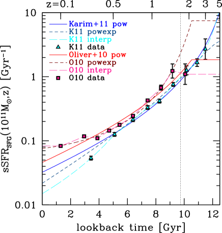
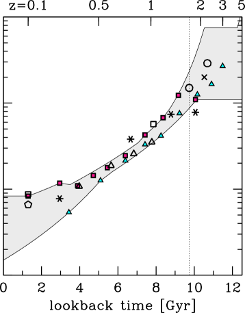
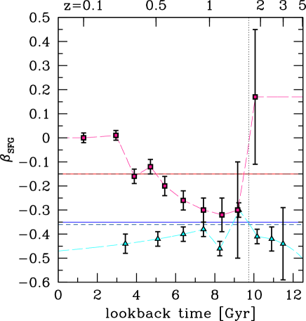
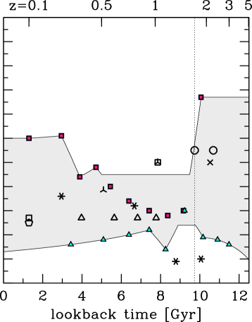
Figure 1.— Top panels: the sSFR of $10^{11}M_{\odot}$ galaxies as a function of redshift. Bottom panels: fits to the powerlaw slope of the SFR-$M_{*}$ relation as a function of redshifts. Left panels: lines show fits to K11 (magenta squares) and O10 (cyan triangle) SFR data (see the legend and numbered text for forms). Right panels: the shaded region marks the area enclosed by our fits (lines) from the left panels. The vertical dotted lines mark ${z_{\rm err}}$ from Figure 2. Points are a compilation of fits to SFR main sequence in redshift bins from a number of groups (hollow triangles: Noeske et al., 2007b; hollow squares: Elbaz et al., 2007; pentagons: Salim et al., 2007; circles: Pannella et al., 2009; crosses: Daddi et al., 2007; three-line cross: Dunne et al., 2009; asterisks: Rodighiero et al., 2010b).

Table 1Fit Parameters for $\psi(M_{\ast},z)$.

Data	$\psi$ Form	$A_{11}(\,{\rm Gyr}^{-1})$	$\alpha$	$\beta$	$\eta$	$\chi^{2}/n_{\rm dof}$
O10	pow (Eq. 1)	0.0460	3.36	$-0.15$	$\cdots$	$22.5^{*}$
O10	powexp (Eq. 2)	0.0759	$-3.14$	$-0.15$	4.02	$9^{*}$
O10	interpolated	$\cdots$	$\cdots$	$\cdots$	$\cdots$	0
K11	pow (Eq. 1 )	0.0324	3.45	$-0.35$	$\cdots$	1.90
K11	powexp (Eq. 2)	0.0219	5.61	$-0.36$	$-0.99$	1.15
K11	interpolated	$\cdots$	$\cdots$	$\cdots$	$\cdots$	0

Note. — Small formal error bars have been omitted, meaningful uncertainties are given by discrepancies between different survey results.

*Fits to specific SFR and $\beta_{\rm SFG}$ are based on the redshift-binned data shown in Figure 1 (not binned by mass).

We integrate fits to the SFR main sequence data to derive MSI-based SFHs. The fits are done separately to the K11 (radio) and the O10 (IR) surveys, thereby providing an estimate of systematic uncertainties in analysis or calibration that are otherwise difficult to estimate. They will also be used to extrapolate measurements to regions of stellar mass and redshift where SFRs are not well constrained (see §2.3.1 for further discussion).

The SFR main sequence is commonly fit to survey data with a power law form in redshift and mass,

$$\psi(M_{\ast},z)=A_{11}\left(\frac{M_{\ast}}{10^{11}M_{\odot}}\right)^{\beta+1}(1+z)^{\alpha}.$$ (1)

Parameters $\alpha$ and $\beta$ are then fit to data in redshift slices. Figure 1 shows the measured sSFR(z) at fixed $M_{\ast}=10^{11}M_{\odot}$ (which is characterized by $A_{11}(1+z)^{\alpha}$; top left) and $\beta(z)$ (bottom left) for SFGs from K11 and O10. The right panels of Figure 1 show data points from many recent surveys, demonstrating that measurements typically occupy the region between K11 and O10.

The $\beta(z)$ parameter in Figure 1 (bottom) shows the extent to which galaxies of different masses assemble at different rates. A negative value means more massive galaxies have smaller specific SFR (${\rm sSFR}\equiv{\rm SFR}/M_{\ast}$) and, therefore, must have formed a larger fraction of their stellar mass at high redshift. This is the “archaeological” form of downsizing, and is the only form of downsizing referred to throughout this paper. Some downsizing is evident from sSFRs – a process also implied by mass function evolution (e.g. Pérez-González et al., 2008; Conroy & Wechsler, 2009). The value of $\beta$ and its evolution vary by survey, but K11 showed that this variation can be largely explained by fluctuations at the edge of mass ranges, and aggressive color selection within the SFR main sequence. Despite the use of a wide variety of different methods and calibrations, there is rough agreement in sSFR observations, in the sense that trends are larger than the scatter between different studies.

In practice, to roughly characterize observations of the SFR main sequence reported by various studies, we fit three different forms to the K11 and O10 SFR data:

1. A power law form (“pow”) that follows Eq. 1 with constant $\alpha$ and $\beta$. The K11 fit is our fiducial model. The O10 fit includes a break to a constant $\psi(M_{\ast})$ at $z\geq 2$.
   

2. A power law times exponential form (“powexp”) that follows Eq. 2 with constant $\alpha$, $\beta$, and $\eta$,

   $$\psi(M_{\ast},z)=A_{11}\left(\frac{M}{10^{11}M_{\odot}}\right)^{\beta+1}(1+z)^{\alpha}e^{\eta z}.$$ (2)

   We thereby account for curvature in Figure 1 (left), and the form allows a formally consistent fit to the K11 SFG data (reduced-$\chi^{2}=1.15$ and $n_{\rm dof}=44$).
   

3. A non-parameteric form that linearly interpolates (in $1+z$) between measurements at different redshifts (“interp”). Outside of the data range, constant and linear extrapolations are used for O10 and K11 respectively.
   

Parameters of the power law and exponential fits are reported in Table 1. For K11 data, we derived the maximum likelihood $\alpha$, $\beta$ and $\eta$ from their average stacked SFR results and errors, binned in both mass and redshift, from their Table 3. For O10, the fits are done separately for the sSFR at $M_{\ast}=10^{11}M_{\odot}$ and $\beta$, based on the points and errors plotted in Figure 1. Fits are plotted as lines in the left panels of Figure 1.

2.3. Reliability of Results

Integration of SFRs to derive SFHs is limited by the availability of SFR main sequence data and the reliability of that data.

2.3.1 Completeness Limits and Extrapolations

The stellar mass at which SFGs are well represented in a dataset is a “completeness” threshold. Our fiducial dataset from K11 reports their $95\%$ statistical completeness threshold – the stellar mass at which the VLA-COSMOS flux limits and source confusion still allow $\mathrel{\raise 1.29167pt\hbox{$>$\kern-7.5pt\lower 4.30554pt\hbox{$\sim$}}}95\%$ of SFGs to be stacked in order to measure SFRs at a given redshift. Strictly speaking completeness limits in K11 make it impossible to derive star formation histories for dwarfs, and limits firm results to massive ($\mathrel{\raise 1.29167pt\hbox{$>$\kern-7.5pt\lower 4.30554pt\hbox{$\sim$}}}10^{10}M_{\odot}$) disks.

However, these limits are conservative, and do not mean that extrapolations are unreliable. On the contrary, there are no clear indications that the tight SFR-$M_{\ast}$ relation falls apart at any mass or redshift. Locally, SFR main sequence trends can be traced across the entire mass function (Brinchmann et al., 2004; Salim et al., 2007; Wyder et al., 2007), with sSFRs rising toward low masses and staying high in dwarf galaxies (e.g.,Lee et al., 2009b; James et al., 2008; Lee et al., 2011). Furthermore, the sequence is also in place at low masses at high redshift (González et al., 2011). More recently, Wuyts et al. (2011a) mapped the sequence to $10^{8}M_{\odot}$ and out to $z=2.5$, finding no obvious change in galaxy properties at any mass or redshift.

Still, data remains limited and hints of a flattening of sSFRs in low mass galaxies and at high redshift have been reported (see K11 for further discussion). Regions where MSI-based star formation histories rely on extrapolated trends are therefore noted with diagonal stripes in figures below.

2.3.2 SFRs at $z>1$ and Consistency with Stellar Mass Density

A number of studies (e.g., Hopkins & Beacom, 2006; Conroy & Wechsler, 2009; Wilkins et al., 2008b; Davé, 2008; Rudnick et al., 2006) have reported that the integral of the cosmic SFR density from $z\mathrel{\raise 1.29167pt\hbox{$>$\kern-7.5pt\lower 4.30554pt\hbox{$\sim$}}}2$ exceeds the growth in stellar mass density relative to what is observed (modulo mass loss). Since measurements of stellar mass density are not subject to the same extrapolation from high mass stars to the bulk of stellar mass, the discrepancy could imply an evolving IMF (e.g, Hopkins & Beacom, 2006; Wilkins et al., 2008a, b; Fardal et al., 2007; Pérez-González et al., 2008; van Dokkum, 2008; Davé, 2008; Gunawardhana et al., 2011; Borch et al., 2006), or a broader failure to properly model the SEDs of these denser, more active, lower metallicity, high-redshift galaxies (e.g., Nordon et al., 2010; Arnouts et al., 2007; although these are increasingly constrained by Herschel, see Elbaz et al., 2011).

In Figure 2, we compare the cosmic SFH from K11 with predictions for the cosmic SFH based on the buildup of stellar mass from a compilation by Wilkins et al. (2008a). Adjusting for their IMF, the K11 points are consistent with the 1-$\sigma$ errors on stellar mass growth predictions below ${z_{\rm err}}\equiv 1.6$ (marked by the vertical dashed line). SFR measurements at $>{z_{\rm err}}$ are discrepant by $>3\sigma$. The stellar populations that are measured, and the corresponding MSI results, cannot be reliably interpreted at $z>{z_{\rm err}}$. MSI-based findings at $z>{z_{\rm err}}$ are therefore noted with dotted shading in figures below.

In the context of past cosmic SFR measurements, K11 findings are on the low end of the Hopkins & Beacom (2006) SFR compilation (see K11 Figure 11), and so indicate that the K11 SFR main sequence is an outlier. On the other hand, K11 is consistent with both past IR data and the growth of stellar mass density in the universe at $z<{z_{\rm err}}$. Moreover, the total star formation observed by K11 since ${z_{\rm err}}$ is similar to the total median star formation inferred by Wilkins et al. (2008a) from the evolution of stellar mass density; applying a correction for a hypothetical evolving IMF would drive K11 measurements out of agreement with SFR data.

While O10 do not measure a cosmic SFH, Rodighiero et al. (2010a) included FIR measurements of the same SWIRE field in their measurements of the cosmic SFH, and K11 report that these measurements are consistent with their findings (within large error bars). The O10 measurements can therefore be considered valid in a similar redshift range, but with more stringent completeness limits because of their shallower SFR observations.

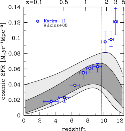
Figure 2.— Cosmic SFR from the K11 SFR sequence data compared to the cosmic SFR expected given the growth of stellar mass measured by Wilkins et al. (2008a). The gray region marks the Wilkins et al. (2008a) $1\sigma$ and $3\sigma$ uncertainty region adjusted from their IMF to a Chabrier (2003) IMF by adding $0.045{\,\rm dex}$ based on the difference in bolometric flux for a bursting population (calculated in PEGASE.2 Fioc & Rocca-Volmerange, 1997) . The vertical line marks the redshift above which SFRs are not well understood (${z_{\rm err}}\equiv 1.6$).

3. The MSI Approach: from Star Formation Rates to Star Formation Histories

With a reliable SFR main sequence in hand at $z\mathrel{\raise 1.29167pt\hbox{$<$\kern-7.5pt\lower 4.30554pt\hbox{$\sim$}}}1.6$, observations can be synthesized through MSI to calculate SFHs, $\Phi(t)$. The evolution of stellar mass in a given galaxy is described by a growth term from the observed SFR and a loss term from the galaxy-wide stellar mass loss rate,

$$\dot{M}_{\ast}(t)=\psi(M_{\ast},z)-\Re(t).$$ (3)

Galaxy-wide mass loss is given by an integral over the fractional mass lost rate ($\dot{f}_{\rm ml}$) from each single age stellar population (SSP) – calculated using the flexible stellar populations synthesis code (v2.0 Conroy & Gunn, 2010; Conroy et al., 2009, or see Leitner & Kravtsov, 2011 for fits),

$$\Re(t)=\int_{t_{0}}^{t}\Phi(t^{\prime})\dot{f}_{\rm ml}(t-t^{\prime})dt^{\prime}.$$ (4)

The SFH of that galaxy is then,

$$\Phi(t)=\psi(M_{\ast}(t),z),$$ (5)

where $\psi$ is a function of the evolving mass. $\Phi(t)$ and $M_{\ast}(t)$ can be thought of as the Lagrangian coordinate tracking a given galaxy, while $\psi$, the SFR main sequence, is the SFR at a fixed Eulerian coordinate in the space of stellar mass and redshift.

For our fiducial choice, galaxies start with boundary condition $M_{\ast 0}\equiv M_{\ast}(z_{\rm obs})$, and trace the median of the SFR main sequence given by Eq. 1 and K11 parameters (in Table 1) as they move back in time and down in stellar mass. Since $\Phi(t)$ is needed to calculate mass loss, but mass loss is needed to solve Eq. 3, a self-consistent solution for $M_{\ast}(t)$ requires iteration. Leitner & Kravtsov (2011) described the simple iteration procedure that is used here to converge on a self-consistent $\Phi(t)$ and $\Re(t)$.

Figure 3 shows mass growth for galaxies including the spread from variation between different SFR main sequence observations (described by fits in §2.2). Appendix A reports analytic approximations. MSI-based SFHs decay almost exponentially after early buildup, and are thus in general agreement with staged-$\tau$ models assumed by Noeske et al. (2007a).

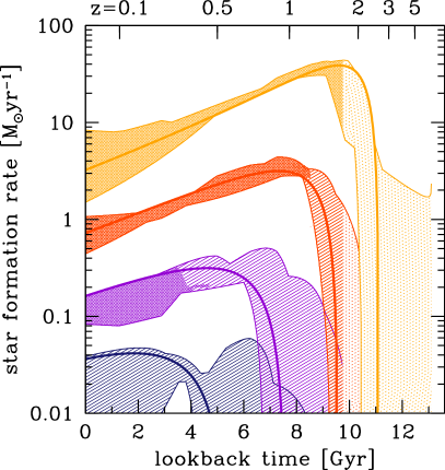
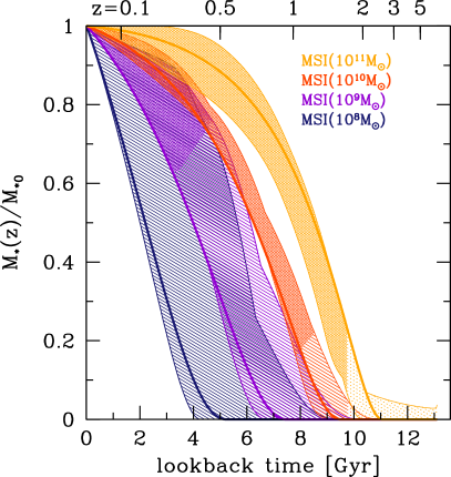
Figure 3.— The SFHs (left) and mass growth (right) from MSI, in galaxies of $M_{\ast 0}=10^{8}M_{\odot}$, $10^{9}M_{\odot}$, $10^{10}M_{\odot}$ and $10^{11}M_{\odot}$. Shaded regions show the variation between SFR main sequence observations and thick lines are fiducial power law SFR main sequence fit to K11 data. Results are shown where SFR main sequence data is robust and complete (cross hatching), extrapolated (diagonal stripes; see completeness discussion in §2.3.1) and compromised by observational uncertainties at $z>{z_{\rm err}}$ (dotted).

3.1. Assessing MSI Complications

In this section we address two issues – mergers and scatter – that were ignored by linking galaxies across SFR observations solely using the median SFR and resulting stellar mass evolution. We find that these issues are probably less important than variations between observations of the SFR main sequence, so readers interested in results can skip to §3.2.

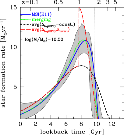
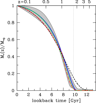
Figure 4.— Changes to MSI-based SFHs (left) and stellar mass growth (right) due to mergers and scatter in SFR-$M_{\ast}$ for SFGs of $M_{\ast 0}=10^{10.5}M_{\odot}$. The gray solid region encompasses the spread between MSI based on K11 and O10 data. The blue line shows the fiducial model to which other lines should be compared. The green dotted lines show averaged MSI merger simulations. The dashed lines show the average of Monte Carlo realizations of the lognormal SFR PDF: black short dashed shows a constant $\Delta_{\,{\rm log}({\rm SFR})}$ across time in a given galaxy and the red long-dashed line shows a constant $\Delta_{\,{\rm log}({\rm SFR})}$ that inverts at $z=1$. The vertical dotted line is at ${z_{\rm err}}$ from Figure 2.

3.1.1 Mergers

MSI is almost insensitive to mergers, both because sSFRs of SFGs are not strongly dependent on mass and because mergers are not common in SFGs at $z<2$. Starting from a $M_{*}(z_{\rm obs})$, galaxies disassemble according to their growth rate, $\dot{M_{\ast}}$, with increasing lookback time. If at some $z_{\rm split}$ there is a merger of ratio $\mu_{\rm mrat}$, the galaxy gets split into two progenitors, both of which continue to contribute to the SFH of the final galaxy. Since sSFRs are mass dependent, the same galaxy grows at a different rate if it is split into progenitors. The ratio of growth in a split to unsplit galaxy is

$$\gamma_{{\rm SFR}}=\frac{1+\mu_{\rm mrat}^{1+\beta}}{\left(1+\mu_{\rm mrat}\right)^{1+\beta}}.$$ (6)

Observations indicate that galaxies downsize ($\beta<0$, see §2.2), so low mass galaxies grow faster and $\gamma_{{\rm SFR}}>1$. Deviations are maximized for rare equal mass mergers, and $\gamma_{{\rm SFR}}\leq 1.3$.

To confirm that merging is not important to stellar mass growth, we couple MSI with merger rate estimates, thereby turning MSI into a empirical generator of merger trees. The merger rate per galaxy, $\nu(M_{\ast}(t),z,\mu_{\rm mrat})$, is tabulated from the semiempirical Halo Occupation Distribution based results of Hopkins et al. (2010) with code that they provide. The (dis-)assembly is then realized with 1,000 Monte Carlo simulations, where each galaxy and its progenitors evolve according to both their observed SFR, $\psi(M_{\ast},t)$, as well as by splitting their stellar mass into progenitor systems at each timestep with probability $\nu(M_{\ast}(t),z,\mu_{\rm mrat})dt$. SFRs and stellar masses are averaged at each timestep and the resulting SFH of the average galaxy due to merging is plotted in Figure 4, along with the same fiducial simulation without mergers. Merging results in very slightly younger SFGs.

Note that this is in no way a physical statement about merger rates or satellites. It is an empirical observation that splitting a SFG into its typical constituent progenitors should not (on average) substantially change the collective growth history of the galaxy.

3.1.2 Scatter in SFR-$M_{\ast}$ and Galaxy Environment

In reality, galaxy SFRs scatter around the median SFR-$M_{\ast}$ value, with approximately lognormal $0.3{\,\rm dex}$ scatter. (Elbaz et al., 2007; Noeske et al., 2007b; Elbaz et al., 2011). Taking $\Delta_{\,{\rm log}({\rm SFR})}$ to be the deviation of a given galaxy from the median relation in some timestep, there are two extreme scenarios for populating that scatter: the $\Delta_{\,{\rm log}({\rm SFR})}$ can be constant across timesteps, or $\Delta_{\,{\rm log}({\rm SFR})}$ can be totally uncorrelated between timesteps. In the correlation coefficient $c_{t}=0$ case (no covariance), average galaxies form stars at the average SFR inside of the lognormal scatter (about the median, $\psi$). Thus the $c_{t}$=0 case closely resembles the fiducial case (with the mean SFR replacing the median). In the case where $c_{t}=1$, active SFGs with $\Delta_{\,{\rm log}({\rm SFR})}>0$ are always active and hence formed a shorter time ago. Correspondingly, less active SFGs ($\Delta_{\,{\rm log}({\rm SFR})}<0$) are always less active and therefore formed at earlier epochs. When averaged, the result is a smeared out SFH as demonstrated in Figure 4.

Observations that parse the breadth of the SFR-$M_{\ast}$ relation for SFGs could implicate one of these scenarios. Insofar as galaxy environment affects accretion history, a second-order correlation of $\Delta_{\,{\rm log}({\rm SFR})}$ with galaxy environment would be the most likely cause of $c_{t}\neq 1$ (see Dutton et al., 2010). A number of groups have found persistent correlations between environment and SFG fraction (e.g., Kauffmann et al., 2004; Cooper et al., 2010; Patel et al., 2011; Sobral et al., 2011; Haines et al., 2007). However, focusing exclusively on SFGs, there are no conclusive indications that $\Delta_{\,{\rm log}({\rm SFR})}$ is significantly driven by environment. At $z\sim 1$, Sobral et al. (2011) found that SFGs form stars $\sim 50\%$ faster in group environments relative to more isolated galaxies of $M_{\ast}<4\times 10^{10}M_{\odot}$ (consistent with Elbaz et al., 2007). Meanwhile, at $z\approx 0.1$, findings are mixed: Peng et al. (2010) discerned no difference between SFRs at fixed mass and varied environment, but Haines et al. (2007) claimed a significant detection of an inverse $\Delta_{\,{\rm log}({\rm SFR})}$-density relation in low mass SFGs and a marginal inverse relation spanning $\sim 0.3{\,\rm dex}$ is also apparent in Popesso et al. (2011, see Figure 15) from their low $0.1\,{\rm Mpc}^{-2}<\Sigma<5\,{\rm Mpc}^{-2}$ to intermediate $5\,{\rm Mpc}^{-2}<\Sigma<30\,{\rm Mpc}^{-2}$ density environments. Clearly it is plausible that $c_{t}=0$, but there is also not enough information to conclude $c_{t}\neq 0$ – that either uniform trends in SFG fraction don’t carry over to the SFR-$M_{\ast}$ relation ($c_{t}=1$), or that SFGs encounter an environmental inversion.

To check for the impact of a (hypothetical) environmental inversion, we re-simulate average MSI SFHs taking the $c_{t}=1$ model from the previous section, and impose an inversion in the amplitude of the scatter for each Monte Carlo simulation at the $z_{\rm invert}=1$ time-step. Figure 4 shows the average of the realizations. This toy model introduces a sharp feature in the average SFH because $z<1$ active isolated galaxies have burned themselves out, leaving a population dominated by relatively passive systems that are relatively active at $z>z_{\rm invert}$. The resulting average mass growth and SFHs are similar to the fiducial model.

Other secondary correlations with $\Delta_{\,{\rm log}({\rm SFR})}$ may further constrain the SFHs of SFGs. Properties, such as galaxy clustering, circular velocity, morphology (e.g., Elbaz et al., 2007; Wuyts et al., 2011a), the evolution SFG number counts, and merging or gas physics, may be used to identify the position of galaxies in the scatter of the SFR main sequence. Each place important priors on SFG growth (see, e.g., Schiminovich et al., 2007; Boissier et al., 2010; Bouché et al., 2010). However, the focus here will be on the implications of consensus SFR observations in a straightforward empirical sense, rather than on embedding the integration in a more physics-driven semi-analytic model. These observations are enough, by themselves, to generate interesting and easily interpreted constraints on galaxy growth.

3.2. The Delayed Assembly of Star-Forming Galaxies

Figure 3 indicates that measuring the early stages of present-day SFG evolution does not require observations of the dawn of galaxy formation. Galaxies observed in the SFR main sequence at high redshifts (e.g., $z>3$) are mostly quiescent and massive by $z=0$, while present-day SFGs appear to have grown most of their mass starting at relatively low redshift ($1<z<2$).

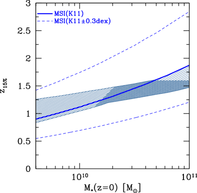
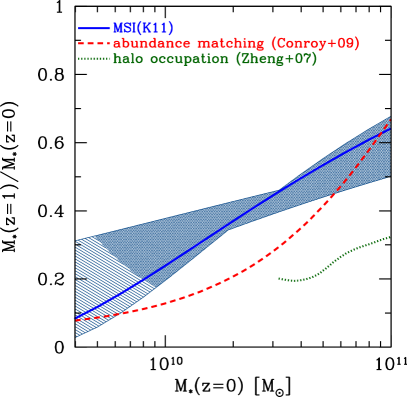
Figure 5.— Left panel: the redshift by which $15\%$ of stellar mass formed in all progenitors of a galaxy from MSI. The shading encompasses variation between K11 and O10 SFR main sequence observations. Striping indicates the reliability of the results as described in Figure 3. The dashed lines show, for reference, the effect of large scatter (or error) in $z_{15\%}$ calculated by adding $\pm 0.3{\,\rm dex}$ to the K11 (thick blue) SFR main sequence. Right panel: the average stellar mass fraction formed by $z=1$ in all progenitors as a function of $z=0$ stellar mass from MSI (blue as above), Abundance Matching (red dashed), and Halo Occupation modeling (green dotted).

3.2.1 Delayed Growth and Relevance to Bulge Formation

SFR main sequence measurements from K11 are deep enough that MSI can follow the growth of stellar mass back to a time when typical SFGs were almost a tenth of their current size. Figure 5 (left) shows the redshift after which MSI indicates average SFGs formed $15\%$ of their stars ($z_{15\%}$). The thin lines in the figure show the effect of a factor of two increase or decrease in the fiducial SFR main sequence; this can be interpreted as illustrating large systematic uncertainties, or a maximal estimate of the $68\%$ scatter in SFHs (i.e., in the $c_{t}=1$ case from §3.1.2, although ignoring ${z_{\rm err}}$).

We focus on $z_{15\%}$ specifically because, for $10^{10}M_{\odot}\mathrel{\raise 1.29167pt\hbox{$<$\kern-7.5pt\lower 4.30554pt\hbox{$\sim$}}}M_{\ast 0}\mathrel{\raise 1.29167pt\hbox{$<$\kern-7.5pt\lower 4.30554pt\hbox{$\sim$}}}5\times 10^{10}$, constraints on $z_{15\%}$ are still data-driven; $z_{15\%}$ results are affected by neither incompleteness, nor disagreement with mass function determinations (${z_{\rm err}}$ from Figure 2). This regime also bears particular relevance for disk galaxy structure and bulge formation in simulations since median observed bulge mass fractions are also $15\%$ (see §5.1 for further discussion). Moreover, focusing on this mass fraction circumvents complicating factors related to bulge formation (e.g., rejuvenated star formation from mergers).

The figure indicates that the peak of star formation in SFGs is delayed relative to high-redshift ($z\mathrel{\raise 1.29167pt\hbox{$>$\kern-7.5pt\lower 4.30554pt\hbox{$\sim$}}}2$) star formers: $85\%$ of stellar mass in many SFGs appears to form after $z\approx 1.5$.

3.2.2 Model Comparisons at $z=1$

Complementary semiempirical methods, based on the galaxy-dark matter connection and simulations, also expect delayed formation of SFGs. Figure 5 (right) shows the fraction of mass formed in galaxies by $z=1$, including results from Abundance Matching (Conroy & Wechsler, 2009, data from their Figure 3) and Halo Occupation analysis (Zheng et al., 2007b, data from their Figure 7). These methods paint galaxies onto dark matter halos in simulations at different epochs according to mass (Abundance Matching) or clustering (Halo Occupation), and then link galaxies across epochs using average dark matter accretion rates onto those dark matter halos during the intervening time. Note that these methods are applied to the galaxy population as a whole, rather than being restricted to SFGs; however, at $M_{\ast}\sim 2\times 10^{10}M_{\odot}$ galaxies transition to being mostly star-forming so the comparison is useful.

Both Abundance Matching and MSI predict lower mass galaxies formed a large portion of their mass after $z\approx 1$, while galaxies of $\sim 10^{11}M_{\odot}$ form most of their mass at higher redshifts. Unexpectedly, however, Conroy & Wechsler (2009) find that even less stellar mass was in place in $z=1$ progenitors than MSI infers – the addition of quiescent galaxies should increase the fraction of stars that form early. The Zheng et al. (2007b) Halo Occupation analysis predicts that even smaller stellar masses were formed before $z=1$ relative to Abundance Matching. For now, systematic errors in the halo-stellar mass relation can account for the $0.3{\,\rm dex}$ tension between different predictions (e.g., from errors on stellar masses and sample variance, see Behroozi et al., 2010; Leauthaud et al., 2011). Indeed, Figure 12 of Behroozi et al. (2010) explicitly shows that Zheng et al. (2007b) halos host fewer stars than most other determinations predict at $z=1$. With tighter constraints, differences from halo-based predictions might be used to infer star formation duty cycles or the possibility of a quenched phase.

4. Comparison of MSI with Fossil Record Analysis

SFHs are more traditionally derived through analysis of a galaxy’s fossil record. This analysis uses either a galaxy’s SED or, in the few local cases where individual stars can be resolved, stellar CMDs. Given an SED $F_{\lambda}$, a stellar census $\Phi(t_{\rm age})$ can be calculated by inverting $F_{\lambda}=\int\Phi(t_{\rm age})S_{\lambda}(t_{\rm age},Z)dt_{\rm age}$, where $S_{\lambda}(t,Z)$ is the SED produced by a SSP in a population synthesis model that includes the metallicity ($Z$) dependent stellar evolution tracks, an IMF, and dust extinction. CMD-based SFHs are similarly derived, but in this case stellar tracks are fit directly instead of being summed over.

Unfortunately, this inverse problem is strongly ill-conditioned; low levels of noise in $F_{\lambda}$ can result in widely varying ages for stellar population, with serious implications for interpretation of SED-based SFHs (see Moultaka et al., 2004; Moultaka & Pelat, 2000; Ocvirk et al., 2006; Cid Fernandes et al., 2005, 2001). Moreover, large statistics can insidiously shrink error bars without improving recoverable resolution. Still, fossil record analysis provides important clues to the growth of mass in galaxies, and is singularly important for measuring the growth of dwarf galaxies where SFR main sequence data is sparse.

4.1. Fossil Record Data: Samples from SDSS and LG+ANGST Dwarfs

Table 2Galaxy Samples

Mass Range $[M_{\odot}]$	${\rm N}_{\rm gal}$	$\langle M_{*}(z_{\rm obs})[M_{\odot}]\rangle$	$\langle z_{\rm obs}\rangle$	$\langle t_{\rm lb}[\,{\rm Gyr}]\rangle$	Source
$M_{\ast}\mathrel{\raise 1.29167pt\hbox{$<$\kern-7.5pt\lower 4.30554pt\hbox{$\sim$}}}10^{8}$	$32$	$4.0\times 10^{7}$	$D<4\,{\rm Mpc}$	$\sim 0$	LG+ANGST W11 dIrr (CMDs)
$10^{8}-10^{8.5}$	$1,115$	$2.1\times 10^{8}$	$0.014$	$0.19$	SDSSSFG (SEDs)
$10^{9}-10^{9.5}$	$12,156$	$2.1\times 10^{9}$	$0.032$	$0.43$	SDSSSFG (SEDs)
$10^{9}-10^{10}$	$39,390$	$5.0\times 10^{9}$	$0.042$	$0.57$	SDSSSFG (SEDs)
$10^{10}-10^{10.5}$	$50,071$	$2.0\times 10^{10}$	$0.070$	$0.92$	SDSSSFG (SEDs)
$10^{10.5}-10^{11}$	$55,780$	$5.8\times 10^{10}$	$0.098$	$1.26$	SDSSSFG (SEDs)
$10^{11}-10^{11.5}$	$29,187$	$1.7\times 10^{11}$	$0.12$	$1.61$	SDSSSFG (SEDs)

In this section, we briefly describe the fossil record samples and analysis methods used. Table 2 summarizes the relevant properties of the sub-samples from which SFHs are derived.

SED-based SFHs (for galaxies with $M_{\ast}>10^{8}M_{\odot}$) are drawn from the VESPA database (Tojeiro et al., 2007, 2009), which stores SFHs from VESPA applied to the spectroscopic sample of the of the SDSS DR7. SFGs are selected from the main galaxy sample (MGS Strauss et al., 2002) using emission line measurements from the general purpose SDSS pipeline, in order to exclude both quiescent galaxies and active galactic nuclei(AGNs). SFGs are required to have ${\rm H\alpha}$ emission detected at $>3\sigma$ significance. If ${\rm H\alpha}$, ${\rm H\beta}$, [${\rm NII}$] ($\lambda 6584$Å), [${\rm OIII}$] ($\lambda 5007$Å) are all detected at $>3\sigma$, then we exclude AGN with a cut in the BPT (Baldwin et al., 1981) diagram from Kauffmann et al. (2003, Eq. 1), $\,{\rm log}\left(\frac{[{\rm OIII}]}{{\rm H\beta}}\right)<0.61\left[\,{\rm log}\left(\frac{[{\rm NII}]}{{\rm H\alpha}}-0.05\right)\right]^{-1}+1.3$, and the requirement that ${\rm NII}/{\rm H\alpha}<0.6$; these cuts are in the spirit of Brinchmann et al. (2004). No efforts have been made to account for galaxy selection, but we note that harsher color cuts (e.g., $U-R<1.5$) selecting more active SFGs had no effect on our results. Placing a low S/N threshold (median S/N$>10$ in all bands with unmasked VESPA $\langle S/N\rangle>20$) also made little difference to SFHs.

The total SFG sample includes about 175,000 galaxies that are split predominantly into three VESPA measured stellar mass bins of $10^{9-10}M_{\odot}$,$10^{10-10.5}M_{\odot}$ and $10^{10.5-11}M_{\odot}$. Two smaller bins, at very low ($10^{8-8.5}M_{\odot}$) and high ($10^{11-11.5}M_{\odot}$) mass, are also recorded. Tojeiro et al. (2007) have shown that VESPA SFHs are consistent with SED analysis from textttMOPED (Heavens et al., 2000), but VESPA also somewhat mitigates over-fitting pitfalls by limiting parameters recovered as advocated by Ocvirk et al. (2006). The sample therefore represents the best SFH analysis of an unsurpassed number of galaxy fossil record observations.

For lower mass dwarf galaxies, we use the SFH compilation by W11 from the ANGST (Dalcanton et al., 2009) measured by Weisz et al. (2011b), and from the LG (Mateo, 1998, Table 1), with CMDs from Dolphin et al. (2005) and Holtzman et al. (2006). The sample is volume limited to $D\mathrel{\raise 1.29167pt\hbox{$<$\kern-7.5pt\lower 4.30554pt\hbox{$\sim$}}}4\,{\rm Mpc}$. Individual stars were resolved and fit with stellar tracks in a CMD. Present-day type and color has little bearing on past SFH beyond the last $1-2\,{\rm Gyr}$ (Weisz et al., 2011b, a), but we will confine our discussion to the relatively isolated LG+ANGST dwarf irregular (dIrr) sample ( W11, ) as a low-mass extension of our normal star-forming sample. The W11 analysis was performed with a Salpeter (1955) IMF, so stellar masses are multiplied by $-0.25{\,\rm dex}$ to convert to a Chabrier (2003) IMF. Their detection limits make IMF differences unimportant for cumulative star formation plots (see W11).

4.2. Uncertainties in Fossil Record Analysis

To account for age errors, we note that SSPs change logarithmically with age intervals and therefore convolve MSI results with a Gaussian filter in log-age. In order to choose a filter width, we note that the SFR weighted average bin size in VESPA is $\sim 0.4{\,\rm dex}$ and covariance between adjacent bins further reduces resolution. For much higher S/N SEDs, Ocvirk et al. (2006) found that disentangling confounding degeneracies, coupled with meager SSP differences, lead to age resolution (full width at half-maximum , ${\Delta_{\rm age}}$) limits of $\mathrel{\raise 1.29167pt\hbox{$>$\kern-7.5pt\lower 4.30554pt\hbox{$\sim$}}}0.8{\,\rm dex}$. Below we present results smoothed with ${\Delta_{\rm age}}=1.0{\,\rm dex}$, but findings are unchanged at $>10^{9}M_{\odot}$ assuming any $0.5{\,\rm dex}<{\Delta_{\rm age}}<1.0{\,\rm dex}$ (see Appendix B for further discussion).

W11 analysis reports broad age bins, such that covariance in simulated data result in uncertainties that are within measurement errors; but, again, this covariance cannot be mitigated by statistics (see their Appendix A and Figure 13, Weisz et al., 2011b). Age errors in CMD analysis can be smaller than in SEDs (see Gallart et al., 2005, for a discussion), but our CMD-related results below are qualitatively unchanged by the error model, so we will use the same smoothing filter for all comparisons.

In addition to resolution, there are substantial systematic uncertainties in stellar population synthesis (SPS) models. VESPA analysis, using both Bruzual & Charlot (hereafter BC03; 2003) and the Maraston (hereafter M05; 2005) SPS models, is shown in plots. Those differences render Poisson error on the mean (of order the point size), irrelevant for all of the SDSS samples in Table 2. For W11 dIrrs, statistical uncertainty is similar to uncertainty between stellar evolution tracks (see their Figure 3). In both cases, error estimates are only qualitative in the sense that they illustrate the difference between models and not the uncertainty in the model parameters.

4.3. Consistency with SDSS SEDs

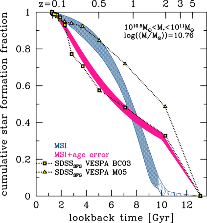
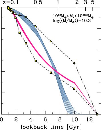
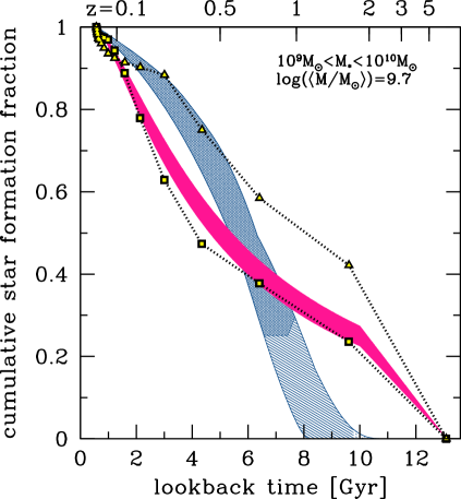
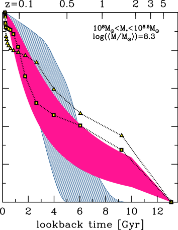
Figure 6.— Cumulative star formation from the SDSS SED modeling (points) and MSI (shaded regions) in four panels for different mass samples. VESPA’s SED analysis of SDSS is shown for the M05 (triangles), and BC03 (squares) population synthesis models. MSI (blue) was initialized with the same average mass and redshift as that of the SDSS samples and then smoothed to mimic age errors (magenta solid). The shading encompasses variation between K11 and O10 SFR main sequence observations. Striping indicates the reliability of the results as described in Figure 3.

Figure 6 shows the average cumulative star formation fraction for VESPA analyzed SDSS SFGs and MSI, divided into panels for different stellar mass bins. MSI models were initialized at the average mass and redshift of the SED comparison sample (Table 2). Black points mark BC03 (squares) and M05 (circles) SPS analysis. These models show substantial differences that are also visible in the (logarithmic) plots of previous studies (e.g., Panter et al., 2007; Tojeiro et al., 2009), likely originating in their different treatment of thermally-pulsing asymptotic giant branch (TP-AGB) stars. These discrepancies remain the subject of active debate (e.g., Maraston, 2005; Conroy & Gunn, 2010; Maraston, 2011; Kriek et al., 2010; MacArthur et al., 2010).

Focusing on the VESPA results, a cursory look suggests that SFGs appear to form stars with an S-curve age distribution. In that case, average present-day SFGs grew rapidly at high redshift ($z>2$) before biding their time at intermediate redshifts – while sSFRs were still $3-10$ times higher than today. Finally, they surge again, forming stars rapidly over the last $1-2\,{\rm Gyr}$.. Such present-day SFGs would have occupied highly biased position in the SFR main sequence, possibly leaving their mark in environmental or structural trends.

However, such a naive interpretation of the data is unwarranted in light of uncertainty in stellar population ages. This uncertainty drives the peak of SFR to spread out, and the logarithmic nature of variations in stellar populations naturally gives rise to that S-curve in cumulative star formation. Specifically, intermediate to old populations shift mass from a high(er) redshift SFR peak to low redshift, while a tail of star formation extends to the beginning of the universe (see figures in Appendix B also). Whatever the SED or CMD quality, the nature of this shape change should be a generic part of properly regularized SED-based analysis. The impact on “true” MSI predictions (blue) is a shift to SFHs that are well matched to the VESPA BC03 SED analysis of SDSS (magenta) at all masses shown.

4.4. Star Formation Trends and Local Dwarfs

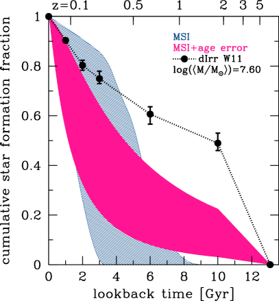
Figure 7.— Same as Figure 6, but black points are W11 CMD-based results for dwarf irregulars (circles). Error bars show statistical uncertainty on the mean, which is similar to systematic variation between different stellar evolution models. MSI trends are extrapolated over this mass range.

For the W11 analysis of dIrr, on the other hand, Figure 7 shows significant differences from extrapolation of MSI below the mass completeness range of SFR surveys. Our simple model of age errors and those errors estimated in W11 are unable to account for these differences. In this regime, MSI predicts excessive downsizing such that dwarfs form most of their mass below $z=1$, while the W11 dIrr galaxies form most of their mass at $z>2$.

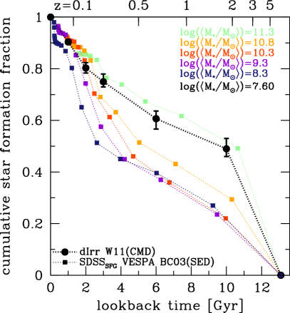
Figure 8.— Cumulative star formation for SDSS SFGs from VESPA BC03 SED modeling in mass bins at $10^{8-8.5}$, $10^{9-9.5}$, $10^{10-10.5}$, $10^{10.5-11}$, and $10^{11-11.5}$, colored (squares) from lightest to darkest respectively, compared to the W11 dIrr sample (black circles). Each mass bin has been rescaled to the linearly interpolated cumulative star formation fraction of the dIrr sample at their epoch of observation. Star formation moves to lower redshift as mass decreases (downsizing), but the dIrrs form more like the most massive sample.

Figure 8 demonstrates the extent of this shift in the context of the VESPA BC03 SED analysis that was matched by MSI trends. The figure shows SFHs in the range $10^{11-11.5}M_{\odot}$, $10^{10-10.5}M_{\odot}$, $10^{9-9.5}M_{\odot}$, and $10^{8-8.5}M_{\odot}$ (from lightest to darkest), plotted over the lower mass W11 dIrrs (most with $M_{\ast}\mathrel{\raise 1.29167pt\hbox{$<$\kern-7.5pt\lower 4.30554pt\hbox{$\sim$}}}10^{8}M_{\odot}$) that are scaled to the linearly interpolated dwarf mass at $\langle z_{\rm obs}\rangle$ of the given sample. Archaeological downsizing is apparent in the purely star-forming sample (as previously noted by, e.g., Cid Fernandes et al., 2005; Asari et al., 2007). Nevertheless, the W11 dIrr galaxies seem to reverse this trend: they assemble more like galaxies of $\sim 10^{11}M_{\odot}$, and deviate strongly from their $\sim 10^{8}M_{\odot}$ siblings analyzed with VESPA and trends in the SFR main sequence.

This is in line with a central conclusion of Weisz et al. (2011a), that the formation of dwarfs in the local volume agrees with the cosmic SFH (which is dominated by massive SFGs, and may be overestimated at $z\mathrel{\raise 1.29167pt\hbox{$>$\kern-7.5pt\lower 4.30554pt\hbox{$\sim$}}}{z_{\rm err}}$), but here we have highlighted that these lowest mass dwarf SFHs seem quite inconsistent with the cosmological downsizing trends found in SFR observations and the SED-based fossil record. A discussion of this shift, and its observational context follows in §5.2.

5. Discussion

In section 3 we showed that MSI indicates late formation of typical SFGs ($z\mathrel{\raise 1.29167pt\hbox{$<$\kern-7.5pt\lower 4.30554pt\hbox{$\sim$}}}2$ and $t_{\rm lb}\mathrel{\raise 1.29167pt\hbox{$<$\kern-7.5pt\lower 4.30554pt\hbox{$\sim$}}}10\,{\rm Gyr}$), then compared the corresponding mass growth with the fossil record in section 4. In this section we place these MSI results in a broader physical and observational context.

5.1. A Simulation Context

Main sequence integration has no connection to galaxy dynamics, so it is interesting to note that its implications align with the trends seen in increasingly successful cosmological simulations. In particular, the late-formation of SFGs suggested by MSI may resolve the (potentially orthogonal) struggle to reproduce the structure of late-type SFGs in simulations.

Current galaxy formation simulations typically convert too much low angular momentum gas into massive bulges. The observed median bulge-to-total (B/T) stellar mass ratio is $15\%$ in bright ($\geq 10^{10}M_{\odot}$) local late-type galaxies (Weinzirl et al., 2009; Gadotti & Kauffmann, 2007), and “bulgeless” disk galaxies are abundant in the local universe (especially dominating at $<10^{10.5}M_{\odot}$ Kormendy et al., 2010; Fisher & Drory, 2011). Such small bulges, embedded in star-forming disks, are rarely reproduced in the current generation of simulations of $M_{\ast 0}\geq 10^{10}M_{\odot}$ galaxies.

Importantly, whatever the physical or numerical mechanisms that drive simulated bulge formation (e.g., Piontek & Steinmetz, 2009; Brook et al., 2011; Governato et al., 2010), state-of-the-art simulations of SFGs consistently produce their excessively massive bulges at $z\mathrel{\raise 1.29167pt\hbox{$>$\kern-7.5pt\lower 4.30554pt\hbox{$\sim$}}}2$ – earlier than MSI indicates $\sim\kern-3.00003pt15\%$ of stellar mass should have assembled. Specifically, Scannapieco et al. (2011) and Stinson et al. (2010) find that their kinematic bulges comprise the majority of each one of their 17 galaxy’s stellar masses; the Scannapieco et al. (2011) bulges form at $z>2$, and the Stinson et al. (2010, Figure 14) non-disk stars also form early. The higher resolution Brooks et al. (2011) sample of 6 massive galaxies with ${\rm B/T}\geq 0.26$ ($\langle{\rm B/T}\rangle=0.44$) also form at least the majority of their mass at $z>1$ (A. Brooks private communication; also see, Brooks et al., 2011, and discussion of sSFRs therein). Guedes et al. (2011) simulated a Milky Way-like disk galaxy with a (photometric) ${\rm B/T}=0.26$, again, with almost all of the bulge mass forming at $z>2$. Suppressed star formation at $z>2$ is responsible for the reduced bulge fraction in a parameter study of a very massive disk in Agertz et al. (2011). Finally, Brook et al. (2011) forms a ${\rm B/T}=0.21$ disk with a SFH that closely matches our fiducial SFH expectation for a $10^{10}M_{\odot}$ system (Figure 3). Delayed formation seems not only achievable in simulations, but also may be important for reproducing typical disk structures.

Intriguingly, two small dwarf galaxy simulations by Governato et al. (2010) manage to form early without forming massive bulges (one is fit by an exponential profile and one has bulge-to-disk ratio of $0.08$). Such simulations may be important for understanding suppressed star formation at low masses and high redshift for all galaxies. They may also lead to a resolution of the unanticipated early growth of W11 dwarfs (but see the next section).

5.2. Resolved and High S/N Observations

The abrupt shift in the CMD-based age distribution of W11 dIrrs compared to SED- and MSI-based SFHs, could instead highlight problems with MSI-, SED-, or CMD-based SFHs. The handful of massive galaxies in Weisz et al. (2011b) form even more of their mass late, with the 0 most massive galaxies in their sample ($M_{\ast}>10^{7.75}M_{\odot}$) reported to have formed $64\pm 0.6\%$ of their stars at $z>2$. That is slightly more $z>2$ star formation than in the lower mass dIrrs ($52^{+4}_{-3}\%$) and makes the nuances of dwarf galaxy formation a less persuasive explanation for the transition to early-forming dwarfs.

Another explanation is simply that the sample is small and biased by the local group overdensity. However, those same W11 dwarfs fit nicely into sSFR trends when measured as part of the larger GALEX-HUGS11 sample of Lee et al. (2009b)(${\rm sSFR}_{\rm K11}\left[10^{7.6}M_{\odot},z=0\right]\approx{\rm sSFR}_{\rm LeeUV}\approx 0.4\,{\rm Gyr}^{-1}$).

Unfortunately, other analyses of resolved populations in SFG disks are limited in number and ability to discern age differences, with too-large error bars on mass formed in a given bin for statistically significant inferences (e.g., Williams et al., 2011). Where any constraint on the $z=2$ divide is reported, results are also mixed: NGC 300 (Gogarten et al., 2010, $2.4\times 10^{10}M_{\odot}$) formed $\sim 70\%$ of its stars at $z>2$, while M33 (Williams et al., 2009; Barker et al., 2007), and NGC 2967 (Williams et al., 2010) may have formed most of their mass at $z<2$.

MacArthur et al. (2009) and Sánchez-Blázquez et al. (2011) recently performed full spectrum fits to high S/N ($\geq 50$) data in the central regions of nearby disk galaxies. While these measurements target the inner disks and bulges of galaxies, the results endorse strikingly old populations for the bulk of stellar mass in galaxy disks. Of their collective 10 galaxies ($M_{\ast}\sim 10^{10}M_{\odot}$) with measurements to the disk scale-length ($r_{d}$), six (I0239, N7495, N7490, N0173, N1358, and N1365) appear to form most, in several cases more than $90\%$, of their stars at $r_{d}$ before $z=2$. The blue regions in Figure 6 shows that galaxies of this mass would be expected to form $10\%$ of their mass over the last $5\,{\rm Gyr}$. If such galaxies form $90\%$ of their entire stellar mass at $z>2$, they would have persisted as massive quenched disks for around $5\,{\rm Gyr}$.

If born out as representative, these results may demand either an important recalibration of SPS models, or a shift in our understanding of where present-day SFGs sit in the SFR main sequence (something not apparent in studies of environment, or the structural main sequence, see §3.1.2). More generally, such extreme examples highlight the value of cross checks between the SFR main sequence and fossil record analysis, especially of the sort recently undertaken by Wuyts et al. (2011b). Clearly, a larger number of high-S/N observations and robust examinations of disk ages will be crucial for a better understanding of SFG growth and of the galaxy fossil record.

6. Summary and Conclusions

We have derived the average growth of stellar mass in present-day SFGs by simple integration of the consensus SFR main sequence under the assumption that SFGs were always SFGs in the past (an approach that we term MSI). Our results regarding average stellar mass growth can be summarized as follows:

• SFGs form late such that only $\sim 15\%$ of the stellar mass in the progenitors of $5\times 10^{9}M_{\odot}\mathrel{\raise 1.29167pt\hbox{$<$\kern-7.5pt\lower 4.30554pt\hbox{$\sim$}}}M_{*0}\mathrel{\raise 1.29167pt\hbox{$<$\kern-7.5pt\lower 4.30554pt\hbox{$\sim$}}}10^{11}M_{\odot}$ galaxies was in place before $z=1-2$ (depending on mass and downsizing).

• It follows that massive SFGs at $z>2$ are not expected to be progenitors of typical SFGs today.

• The effect of mergers on MSI results was found to be negligible based on semiempirical merger trees generated in the MSI framework.

• Similarly, there is no clear evidence that the way SFGs occupy the distribution of SFRs in the SFR$-M_{*}$ relation significantly alter MSI results.

• Accurate analytic approximations to average SFHs derived from MSI are presented in Appendix A.

Moreover, the delayed formation of SFGs implied by our analysis (but first noted in the stage-$\tau$ models of Noeske et al., 2007a) was found to be consistent with observations of the evolution of stellar mass in the universe, is also implied by halo-based semiempirical methods (Conroy & Wechsler, 2009; Zheng et al., 2007a), and fits well in the context of increasingly successful cosmological simulations.

When comparing MSI-based SFHs to those inferred from the fossil record, we found that,

• Expected age uncertainties in SED-based analysis cause a characteristic shape distortion in derived SFHs.

• SED analysis of SDSS SFGs could be reconciled with MSI after accounting for these expected age uncertainties.

• Local dwarf galaxies with $\langle M_{*}\rangle<10^{8}$, on the other hand, were found to depart from MSI downsizing extrapolations, with SFHs resembling those of $10^{11}M_{\odot}$ galaxies.

We stressed that the last point may reflect systematic errors in population synthesis models rather than a physical transition. For a handful of cases, CMD and high S/N SED analysis of more massive galaxies suggests more early star formation than inferred from MSI. A larger sample of SFGs is greatly needed and it is clear from our SDSS comparison that a full understanding age uncertainties is crucial for interpretation of that data. It will be interesting to see how improved SED modeling and larger data sets can be accommodated in the SFR main sequence.

Appendix A Analytic SFHs

With a few approximations, accurate analytic formulae for average SFH and stellar mass growth based on SFR observations can be derived. Since these may be useful for tying chemical evolution or SPS models to SFR main sequence measurements (e.g., Wuyts et al., 2011b) or for simulation comparisons, they are provided below.

First, in the concordance cosmology, the expansion factor is linear as a function of lookback time to $<5\%$ accuracy until $t_{\rm lb}\approx 12.5\,{\rm Gyr}$ or $z\approx 4$,

$$(1+z)\approx(1-\lambda_{a}t_{\rm lb})^{-1},$$ (A1)

where $\lambda_{a}=(1-a(t_{\rm lin}))/t_{\rm lin}$ and we take $t_{\rm lin}=12\,{\rm Gyr}$ so that $\lambda_{a}=0.064\,{\rm Gyr}^{-1}$ in our cosmology. Rewriting Eq. 3 in terms of the stellar mass fraction formed $f_{\ast}(t)\equiv\frac{M_{\ast}(t)}{M_{\ast 0}}$, and with $R(t)\equiv\Re(t)/\Phi(t)$ being the fraction of the current SFR returned to the ISM by stellar mass loss, then, for a power law fit to the SFR main sequence (Eq. 1),

$$\dot{f_{\ast}}(t)=\left[1-R(t)\right]\dot{f}_{0}{f_{\ast}(t)}^{1+\beta}(1-\lambda_{a}t)^{-\alpha},$$ (A2)

where $\dot{f}_{0}=\frac{A_{11}}{M_{\ast 0}}\left(\frac{M_{\ast 0}}{10^{11}M_{\odot}}\right)^{\beta+1}$. Taking $R(t)=0.45$ and integrating for $f_{\ast}$,

$$f_{\ast}(t)=\left[1+\frac{\beta}{(\alpha-1)}\frac{\dot{f}_{0}\left[1-R(t)\right]}{\lambda_{a}}\left[(1+z)^{\alpha-1}-1\right]\right]^{-\frac{1}{\beta}}.$$ (A3)

Then, plugging Eq. A3 into Eq. A2, analytic SFHs, $\Phi(t)=M_{\ast 0}\dot{f}_{\ast}(t)/\left[1-R(t)\right]$, can be synthesized from a power law $\psi$:

$$\Phi(t)=M_{\ast 0}\dot{f}_{0}(1+z)^{\alpha}\left[1+\frac{\beta}{(\alpha-1)}\frac{\dot{f}_{0}\left[1-R(t)\right]}{\lambda_{a}}\left[(1+z)^{\alpha-1}-1\right]\right]^{-\frac{1+\beta}{\beta}}.$$ (A4)

$\alpha$ and $\beta$ parameters can be found in Table 1 (under the “pow” form) and are commonly reported with SFR sequence observations. Any broken power law in $\alpha$ or $\beta$ is a simple extension (e.g., for a flattening of $\alpha$ at $z\approx 2$ or a flattening of $\beta$ in dwarfs).

The dashed gray line in Figure 9 shows analytic SFHs and $f_{\ast}(t)$ for constant $R(t)=0.45$. Results are in good agreement with the full MSI procedure, but late mass growth is overestimated in massive galaxies because mass loss from old stars is not properly accounted for when assuming a constant return fraction (see Leitner & Kravtsov, 2011).

As a first order correction for massive galaxies, the return fraction can be decomposed into a constant term from young stars, $R_{0}$, and a term related to accumulated old stellar mass. The relative fraction of gas returned by old stars is roughly proportional to a galaxy’s age $(t_{\rm form}-t_{\rm lb})$ (i.e., amount of stellar mass if star formation were constant since $t_{\rm form}$) calibrated to a reference return fraction, $R_{11}$, in a galaxy of $10^{11}M_{\odot}$ with ${t_{\rm form}}_{11}$. Then

$$R(t_{\rm lb})=R_{0}\left(1+\frac{\left(t_{\rm form}-t_{\rm lb}\right)}{t_{\rm form}}\frac{t_{\rm form}}{{t_{\rm form}}_{11}}\frac{R_{11}}{R_{0}}\right),$$ (A5)

assigning $f_{\ast\rm form}(t_{\rm form})\equiv 0.1$:

$$\lambda_{a}t_{\rm form}=1-\left[1-\frac{(\alpha-1)}{\beta}\frac{\lambda_{a}(1-f_{\ast\rm form}^{-\beta})}{\dot{f}_{0}\left[1-R(t)\right]}\right]^{-\frac{1}{\alpha-1}}.$$ (A6)

We calculate $t_{\rm form}$ values using $R(t)=0.45$, and plug those values into Eq, A5, with $R_{0}=0.45$ and $R_{11}=0.30$. Inserting the full return rate from Eq. A5 into Eq. A3 results in the $\Phi(t)$ and $f_{\ast}(t)$ values plotted (dotted lines) over the full MSI models (solid lines) in Figure 9. The $f_{\ast}$ and SFH approximations are accurate to a couple of percent of the final stellar mass (i.e., $20\%$ error when the galaxy is $10\%$ of $M_{\ast 0}$). The same correction are equally accurate for the O10 parameterization.

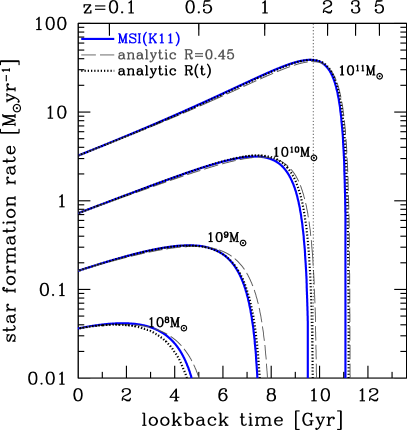
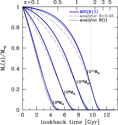
Figure 9.— SFHs (left) and mass growth (right) from MSI, in galaxies of $M_{\ast 0}=10^{8}M_{\odot}$, $10^{9}M_{\odot}$, $10^{10}M_{\odot}$ and $10^{11}M_{\odot}$. Calculations are shown for the fiducial SFR fit (K11) using the full MSI approach (blue lines), and analytic approximations with $\Re=0.45$ (gray long-dashed), and $\Re(t)$ (black dotted; given by Eq. A5). Vertical dotted lines are ${z_{\rm err}}$ from Figure 2.

Appendix B Notes on Age Resolution

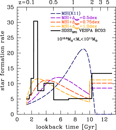
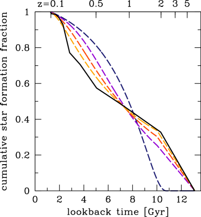
Figure 10.— SFH (left) and cumulative star formation fraction (right) for SDSS SFGs of $10^{10.5-11}M_{\odot}$ from VESPA analyzed with Bruzual & Charlot (2003) (solid black), compared to MSI (dashed) with varied age resolution (see legend). MSI starts with the same average mass and look back time as the SDSS sample. The first 7 VESPA age-bins were combined to remove artifacts.

In §4.3 we show that SFHs based on the fossil record can be misleading, particularly about early galaxy growth. The root of this claim is the consensus view that the maximum reliable precision of age determinations in SED-analysis is low ($>0.5{\,\rm dex}$ Ocvirk et al., 2006; Walcher et al., 2011; Cid Fernandes, 2007). Our solution is a similarly uncontroversial smoothing of the SFH to mimic age errors. The result, however, is a notable change in the shape of SFHs that brings VESPA results into line with cosmological SFR trends (i.e., the SFR main sequence). In light of the importance of noise modeling to this result, a discussion of age errors is prudent. For guidance, we rely on Ocvirk et al. (2006) who carried out a thorough simulation campaign to quantify the noise properties of SSPs and full spectrum fitting in PEGASE-HR (Le Borgne et al., 2004) with implications for interpretation of any optical SED inversion. This section provides a short summary of the issue, and a discussion of how it pertains to VESPA results.

Modeling the intrinsic SEDs of galaxies involves the conflicting goals of (1) finding a stellar population (metallicity and extinction) that generates a good fit to SED, and (2) not letting that population be shaped by noise in SEDs. Even fitting in the absence of noise is not clear cut because stellar evolution models do not match all of the observed features in galaxy spectra (see e.g., Tojeiro et al., 2007; Panter et al., 2007; Cid Fernandes et al., 2005; Conroy & Gunn, 2010; Walcher et al., 2011) and the calibration of important pieces of stellar evolution (e.g., TP-AGB stars at long wavelengths: Maraston, 2005; Conroy & Gunn, 2010; Maraston, 2011; Kriek et al., 2010 ; stellar abundance: Panter et al., 2007; MacArthur et al., 2009; IMF, etc.) are ongoing. Ocvirk et al. (2006) found that noise calibrated into the model PEGASE-HR spectra themselves place a fundamental floor of $\sim 0.4{\,\rm dex}$ on age recovery for even the highest S/N spectra. They also found that noise in SEDs typical of SDSS spectra (S/N$\approx 20$ per $\sim 3$Å pixel in the unmasked VESPA range) renders differences between simple SSPs unrecoverable within $\sim 0.5{\,\rm dex}$. Any smaller-scale time information derived from SEDs must come from noise, improved modeling, or the use of a larger spectral range. Moreover, these resolutions are further broadened when considering non-SSPs with uncertain metallicities, extinction and physical effects (e.g., Wuyts et al., 2009). Regularization techniques can be used to assign resolution to solutions so that they are consistent with these noise limitations and primarily responsive to signal.

VESPA attempts to regularize the stellar population solution using the general procedure of Ocvirk et al. (2006, STECMAP), but adaptively refined logarithmic age bins for basis vectors. Given a solution basis of age bins, metallicities and extinction, VESPA estimates the contribution of noise to the coefficients (parameters) that multiply the solution basis. The number of parameters used to describe the solution should be $\leq\kappa$, the number of coefficients that are not noise dominated (see Tojeiro et al., 2007, §2.2.2 ). Then, to select an appropriate age basis, the bins that contribute the most to the total flux in the model are iteratively refined until they reach the maximum ${\Delta_{\rm age}}\approx 0.2{\,\rm dex}$ resolution. $\kappa$ is recalculated at each iteration. Finally, the chosen solution is the most refined solution that has fewer non-zero flux age bins (and other model parameters) than $\kappa$.

Contrary to the results of (Ocvirk et al., 2006) that ${\Delta_{\rm age}}<0.4{\,\rm dex}$ is not achievable, VESPA regularly refines to its highest resolution ${\Delta_{\rm age}}\approx 0.2{\,\rm dex}$. A full exploration of this discrepancy is well beyond the scope of this paper, but one plausible explanation is that, since bins containing no flux do not count toward the parameter limit, $\kappa$, VESPA favors higher frequency solution variations than can be robustly extracted (R. Tojeiro, private communications). In contrast, STECMAP preferentially weights smooth basis vectors for their solutions using well tested algorithms to eliminate artifacts. Although it is not clear that the smoothed STECMAP basis is ideal (as noted by Ocvirk et al., 2006), the VESPA basis appears to be to aggressive. Ill conditioning of the inversion means there is no way to know exactly how noise-modified light gets interpreted into a stellar age spread.

Artifacts are to be expected but, supported by covariance primarily between adjacent bins in VESPA tests, we assume that VESPA will mimic the STECMAP regularization. That regularization favors small gradients in $\,{\rm log}(t_{\rm age})$, finds little bias in $\langle\,{\rm log}(t_{\rm age})\rangle$, and almost constant logarithmic resolution $\pm{\Delta_{\rm age}}/2$ about any median log-age value. In this case a log-age Gaussian convolution with constant full width half max (${\Delta_{\rm age}}$) is the obvious choice for a noise-model. The $1{\,\rm dex}$ resolution, as noted in §4.2, is motivated both by the (Tojeiro et al., 2007) covariance between adjacent bins and the typical mass-weighted size of the bins. The convolution preserves $\langle\,{\rm log}(t_{\rm age})\rangle$ and biases $\langle t_{\rm age}\rangle$, depending on how the $t_{\rm age}$ distribution is limited by cosmology.

Figure 10 demonstrates that the ${\Delta_{\rm age}}$ size for massive SFGs, does not qualitatively alter our results. The figure shows the SFH and cumulative star formation recovered by VESPA for galaxies of $10^{10-10.5}M_{\odot}$ using Bruzual & Charlot (2003) analysis binned and averaged at the highest age resolution (black solid line), compared to MSI models (dashed) smoothed in log-age with ${\Delta_{\rm age}}=0,0.5,0.75$ and $1{\,\rm dex}$. The first seven VESPA bins were combined to hide (dramatic) artifacts in these bins The S-curve noted in §4.3 grows (right) with increasing ${\Delta_{\rm age}}$ and, correspondingly, the SFH peak flattens (left).

References

- Abazajian et al. (2009) Abazajian, K. N., et al. 2009, ApJS, 182, 543
- Agertz et al. (2011) Agertz, O., Teyssier, R., & Moore, B. 2011, MNRAS, 410, 1391
- Arnouts et al. (2007) Arnouts, S., et al. 2007, A&A, 476, 137
- Asari et al. (2007) Asari, N. V., Cid Fernandes, R., Stasińska, G., Torres-Papaqui, J. P., Mateus, A., Sodré, L., Schoenell, W., & Gomes, J. M. 2007, MNRAS, 381, 263
- Baldwin et al. (1981) Baldwin, J. A., Phillips, M. M., & Terlevich, R. 1981, PASP, 93, 5
- Barker et al. (2007) Barker, M. K., Sarajedini, A., Geisler, D., Harding, P., & Schommer, R. 2007, AJ, 133, 1138
- Barro et al. (2011) Barro, G., et al. 2011, ApJS, 193, 30
- Bauer et al. (2011) Bauer, A. E., Conselice, C. J., Pérez-González, P. G., Grützbauch, R., Bluck, A. F. L., Buitrago, F., & Mortlock, A. 2011, MNRAS, 417, 289
- Bauer et al. (2005) Bauer, A. E., Drory, N., Hill, G. J., & Feulner, G. 2005, ApJ, 621, L89
- Behroozi et al. (2010) Behroozi, P. S., Conroy, C., & Wechsler, R. H. 2010, ApJ, 717, 379
- Bell (2003) Bell, E. F. 2003, ApJ, 586, 794
- Bell et al. (2007) Bell, E. F., Zheng, X. Z., Papovich, C., Borch, A., Wolf, C., & Meisenheimer, K. 2007, ApJ, 663, 834
- Boissier et al. (2010) Boissier, S., Buat, V., & Ilbert, O. 2010, A&A, 522, A18+
- Borch et al. (2006) Borch, A., et al. 2006, A&A, 453, 869
- Bothwell et al. (2011) Bothwell, M. S., et al. 2011, MNRAS, 415, 1815
- Bouché et al. (2010) Bouché, N., et al. 2010, ApJ, 718, 1001
- Bourne et al. (2011) Bourne, N., Dunne, L., Ivison, R. J., Maddox, S. J., Dickinson, M., & Frayer, D. T. 2011, MNRAS, 410, 1155
- Brinchmann et al. (2004) Brinchmann, J., Charlot, S., White, S. D. M., Tremonti, C., Kauffmann, G., Heckman, T., & Brinkmann, J. 2004, MNRAS, 351, 1151
- Brook et al. (2011) Brook, C. B., Stinson, G., Gibson, B. K., Roškar, R., Wadsley, J., & Quinn, T. 2011, MNRAS, 1697
- Brooks et al. (2011) Brooks, A. M., et al. 2011, ApJ, 728, 51
- Bruzual & Charlot (2003) Bruzual, G., & Charlot, S. 2003, MNRAS, 344, 1000
- Buat et al. (2010) Buat, V., et al. 2010, MNRAS, 409, L1
- Chabrier (2003) Chabrier, G. 2003, PASP, 115, 763
- Chary & Elbaz (2001) Chary, R., & Elbaz, D. 2001, ApJ, 556, 562
- Cid Fernandes (2007) Cid Fernandes, R. 2007, in IAU Symposium, Vol. 241, IAU Symposium, ed. A. Vazdekis & R. F. Peletier, 461–469
- Cid Fernandes et al. (2005) Cid Fernandes, R., Mateus, A., Sodré, L., Stasińska, G., & Gomes, J. M. 2005, MNRAS, 358, 363
- Cid Fernandes et al. (2001) Cid Fernandes, R., Sodré, L., Schmitt, H. R., & Leão, J. R. S. 2001, MNRAS, 325, 60
- Conroy & Gunn (2010) Conroy, C., & Gunn, J. E. 2010, ApJ, 712, 833
- Conroy et al. (2009) Conroy, C., Gunn, J. E., & White, M. 2009, ApJ, 699, 486
- Conroy & Wechsler (2009) Conroy, C., & Wechsler, R. H. 2009, ApJ, 696, 620
- Cooper et al. (2010) Cooper, M. C., et al. 2010, MNRAS, 409, 337
- Cowie & Barger (2008) Cowie, L. L., & Barger, A. J. 2008, ApJ, 686, 72
- Cowie et al. (1996) Cowie, L. L., Songaila, A., Hu, E. M., & Cohen, J. G. 1996, AJ, 112, 839
- Daddi et al. (2007) Daddi, E., et al. 2007, ApJ, 670, 156
- Dalcanton et al. (2009) Dalcanton, J. J., et al. 2009, ApJS, 183, 67
- Damen et al. (2009) Damen, M., Labbé, I., Franx, M., van Dokkum, P. G., Taylor, E. N., & Gawiser, E. J. 2009, ApJ, 690, 937
- Davé (2008) Davé, R. 2008, MNRAS, 385, 147
- Dolphin et al. (2005) Dolphin, A. E., Weisz, D. R., Skillman, E. D., & Holtzman, J. A. 2005, arXiv:astro-ph/0506430
- Drory & Alvarez (2008) Drory, N., & Alvarez, M. 2008, ApJ, 680, 41
- Dunne et al. (2009) Dunne, L., et al. 2009, MNRAS, 394, 3
- Dutton et al. (2010) Dutton, A. A., van den Bosch, F. C., & Dekel, A. 2010, MNRAS, 405, 1690
- Elbaz et al. (2007) Elbaz, D., et al. 2007, A&A, 468, 33
- Elbaz et al. (2010) —. 2010, A&A, 518, L29+
- Elbaz et al. (2011) —. 2011, A&A, 533, A119
- Fadda et al. (2006) Fadda, D., et al. 2006, AJ, 131, 2859
- Fardal et al. (2007) Fardal, M. A., Katz, N., Weinberg, D. H., & Davé, R. 2007, MNRAS, 379, 985
- Feulner et al. (2005) Feulner, G., Gabasch, A., Salvato, M., Drory, N., Hopp, U., & Bender, R. 2005, ApJ, 633, L9
- Fioc & Rocca-Volmerange (1997) Fioc, M., & Rocca-Volmerange, B. 1997, A&A, 326, 950
- Fisher & Drory (2011) Fisher, D. B., & Drory, N. 2011, ApJ, 733, L47+
- Gadotti & Kauffmann (2007) Gadotti, D., & Kauffmann, G. 2007, in IAU Symposium, Vol. 241, IAU Symposium, ed. A. Vazdekis & R. F. Peletier, 507–508
- Gallart et al. (2005) Gallart, C., Zoccali, M., & Aparicio, A. 2005, ARA&A, 43, 387
- Gogarten et al. (2010) Gogarten, S. M., et al. 2010, ApJ, 712, 858
- González et al. (2011) González, V., Labbé, I., Bouwens, R. J., Illingworth, G., Franx, M., & Kriek, M. 2011, ApJ, 735, L34
- Governato et al. (2010) Governato, F., et al. 2010, Nature, 463, 203
- Graham (2011) Graham, A. W. 2011, ArXiv e-prints
- Guedes et al. (2011) Guedes, J., Callegari, S., Madau, P., & Mayer, L. 2011, ApJ, 742, 76
- Gunawardhana et al. (2011) Gunawardhana, M. L. P., et al. 2011, MNRAS, 415, 1647
- Haines et al. (2007) Haines, C. P., Gargiulo, A., La Barbera, F., Mercurio, A., Merluzzi, P., & Busarello, G. 2007, MNRAS, 381, 7
- Heavens et al. (2000) Heavens, A. F., Jimenez, R., & Lahav, O. 2000, MNRAS, 317, 965
- Holtzman et al. (2006) Holtzman, J. A., Afonso, C., & Dolphin, A. 2006, ApJS, 166, 534
- Hopkins & Beacom (2006) Hopkins, A. M., & Beacom, J. F. 2006, ApJ, 651, 142
- Hopkins et al. (2009) Hopkins, P. F., et al. 2009, MNRAS, 397, 802
- Hopkins et al. (2010) —. 2010, ApJ, 715, 202
- Hunter et al. (2011) Hunter, D. A., Elmegreen, B. G., Oh, S.-H., Anderson, E., Nordgren, T. E., Massey, P., Wilsey, N., & Riabokin, M. 2011, AJ, 142, 121
- Ilbert et al. (2010) Ilbert, O., et al. 2010, ApJ, 709, 644
- Ivison et al. (2010) Ivison, R. J., et al. 2010, A&A, 518, L31+
- James et al. (2008) James, P. A., Prescott, M., & Baldry, I. K. 2008, A&A, 484, 703
- Jarvis et al. (2010) Jarvis, M. J., et al. 2010, MNRAS, 409, 92
- Karim et al. (2011) Karim, A., et al. 2011, ApJ, 730, 61
- Kauffmann et al. (2004) Kauffmann, G., White, S. D. M., Heckman, T. M., Ménard, B., Brinchmann, J., Charlot, S., Tremonti, C., & Brinkmann, J. 2004, MNRAS, 353, 713
- Kauffmann et al. (2003) Kauffmann, G., et al. 2003, MNRAS, 341, 54
- Kennicutt (1998) Kennicutt, Jr., R. C. 1998, ApJ, 498, 541
- Kormendy et al. (2010) Kormendy, J., Drory, N., Bender, R., & Cornell, M. E. 2010, ApJ, 723, 54
- Kriek et al. (2011) Kriek, M., van Dokkum, P. G., Whitaker, K. E., Labbe, I., Franx, M., & Brammer, G. B. 2011, arXiv:1103.0279
- Kriek et al. (2010) Kriek, M., et al. 2010, ApJ, 722, L64
- Le Borgne et al. (2004) Le Borgne, D., Rocca-Volmerange, B., Prugniel, P., Lançon, A., Fioc, M., & Soubiran, C. 2004, A&A, 425, 881
- Leauthaud et al. (2011) Leauthaud, A., et al. 2011, arXiv:1104.0928
- Lee et al. (2009a) Lee, J. C., Kennicutt, Jr., R. C., Funes, S. J. J. G., Sakai, S., & Akiyama, S. 2009a, ApJ, 692, 1305
- Lee et al. (2009b) Lee, J. C., et al. 2009b, ApJ, 706, 599
- Lee et al. (2011) —. 2011, ApJS, 192, 6
- Leitner & Kravtsov (2011) Leitner, S. N., & Kravtsov, A. V. 2011, ApJ, 734, 48
- Lonsdale et al. (2004) Lonsdale, C., et al. 2004, ApJS, 154, 54
- Lonsdale et al. (2003) Lonsdale, C. J., et al. 2003, PASP, 115, 897
- MacArthur et al. (2009) MacArthur, L. A., González, J. J., & Courteau, S. 2009, MNRAS, 395, 28
- MacArthur et al. (2010) MacArthur, L. A., McDonald, M., Courteau, S., & Jesús González, J. 2010, ApJ, 718, 768
- Magdis et al. (2010) Magdis, G. E., Elbaz, D., Daddi, E., Morrison, G. E., Dickinson, M., Rigopoulou, D., Gobat, R., & Hwang, H. S. 2010, ApJ, 714, 1740
- Mao et al. (2011) Mao, M. Y., Huynh, M. T., Norris, R. P., Dickinson, M., Frayer, D., Helou, G., & Monkiewicz, J. A. 2011, ApJ, 731, 79
- Maraston (2005) Maraston, C. 2005, MNRAS, 362, 799
- Maraston (2011) —. 2011, arXiv:1104.0022
- Mateo (1998) Mateo, M. L. 1998, ARA&A, 36, 435
- Mateus et al. (2006) Mateus, A., Sodré, L., Cid Fernandes, R., Stasińska, G., Schoenell, W., & Gomes, J. M. 2006, MNRAS, 370, 721
- Meurer et al. (2006) Meurer, G. R., et al. 2006, ApJS, 165, 307
- Moultaka et al. (2004) Moultaka, J., Boisson, C., Joly, M., & Pelat, D. 2004, A&A, 420, 459
- Moultaka & Pelat (2000) Moultaka, J., & Pelat, D. 2000, MNRAS, 314, 409
- Noeske et al. (2007a) Noeske, K. G., et al. 2007a, ApJ, 660, L47
- Noeske et al. (2007b) —. 2007b, ApJ, 660, L43
- Nordon et al. (2010) Nordon, R., et al. 2010, A&A, 518, L24+
- Ocvirk et al. (2006) Ocvirk, P., Pichon, C., Lançon, A., & Thiébaut, E. 2006, MNRAS, 365, 46
- Oliver et al. (2010) Oliver, S., et al. 2010, MNRAS, 405, 2279
- Pannella et al. (2009) Pannella, M., et al. 2009, ApJ, 698, L116
- Panter et al. (2007) Panter, B., Jimenez, R., Heavens, A. F., & Charlot, S. 2007, MNRAS, 378, 1550
- Papovich et al. (2011) Papovich, C., Finkelstein, S. L., Ferguson, H. C., Lotz, J. M., & Giavalisco, M. 2011, MNRAS, 412, 1123
- Patel et al. (2011) Patel, S. G., Kelson, D. D., Holden, B. P., Franx, M., & Illingworth, G. D. 2011, ApJ, 735, 53
- Peng et al. (2011) Peng, Y., Lilly, S. J., Renzini, A., & Carollo, M. 2011, arXiv:1106.2546
- Peng et al. (2010) Peng, Y.-j., et al. 2010, ApJ, 721, 193
- Pérez-González et al. (2005) Pérez-González, P. G., et al. 2005, ApJ, 630, 82
- Pérez-González et al. (2008) —. 2008, ApJ, 675, 234
- Piontek & Steinmetz (2009) Piontek, F., & Steinmetz, M. 2009, arXiv:0909.4167
- Popesso et al. (2011) Popesso, P., et al. 2011, A&A, 532, A145
- Quintero et al. (2004) Quintero, A. D., et al. 2004, ApJ, 602, 190
- Renzini (2009) Renzini, A. 2009, MNRAS, 398, L58
- Richards et al. (2009) Richards, J. W., Freeman, P. E., Lee, A. B., & Schafer, C. M. 2009, MNRAS, 399, 1044
- Roberts & Haynes (1994) Roberts, M. S., & Haynes, M. P. 1994, ARA&A, 32, 115
- Rodighiero et al. (2010a) Rodighiero, G., et al. 2010a, A&A, 515, A8+
- Rodighiero et al. (2010b) —. 2010b, A&A, 518, L25+
- Rodighiero et al. (2011) —. 2011, arXiv:1108.0933
- Rudnick et al. (2006) Rudnick, G., et al. 2006, ApJ, 650, 624
- Salim et al. (2007) Salim, S., et al. 2007, ApJS, 173, 267
- Salpeter (1955) Salpeter, E. E. 1955, ApJ, 121, 161
- Sánchez-Blázquez et al. (2011) Sánchez-Blázquez, P., Ocvirk, P., Gibson, B. K., Pérez, I., & Peletier, R. F. 2011, MNRAS, 415, 709
- Sargent et al. (2010a) Sargent, M. T., et al. 2010a, ApJ, 714, L190
- Sargent et al. (2010b) —. 2010b, ApJS, 186, 341
- Scannapieco et al. (2011) Scannapieco, C., White, S. D. M., Springel, V., & Tissera, P. B. 2011, arXiv:1105.0680
- Schiminovich et al. (2007) Schiminovich, D., et al. 2007, ApJS, 173, 315
- Schmidt (1959) Schmidt, M. 1959, ApJ, 129, 243
- Sobral et al. (2011) Sobral, D., Best, P. N., Smail, I., Geach, J. E., Cirasuolo, M., Garn, T., & Dalton, G. B. 2011, MNRAS, 411, 675
- Stinson et al. (2010) Stinson, G. S., Bailin, J., Couchman, H., Wadsley, J., Shen, S., Nickerson, S., Brook, C., & Quinn, T. 2010, MNRAS, 408, 812
- Strauss et al. (2002) Strauss, M. A., et al. 2002, AJ, 124, 1810
- Takeuchi et al. (2005) Takeuchi, T. T., Buat, V., & Burgarella, D. 2005, A&A, 440, L17
- Takeuchi et al. (2010) Takeuchi, T. T., Buat, V., Heinis, S., Giovannoli, E., Yuan, F.-T., Iglesias-Páramo, J., Murata, K. L., & Burgarella, D. 2010, A&A, 514, A4+
- Tojeiro et al. (2007) Tojeiro, R., Heavens, A. F., Jimenez, R., & Panter, B. 2007, MNRAS, 381, 1252
- Tojeiro et al. (2009) Tojeiro, R., Wilkins, S., Heavens, A. F., Panter, B., & Jimenez, R. 2009, ApJS, 185, 1
- van Dokkum (2008) van Dokkum, P. G. 2008, ApJ, 674, 29
- Walcher et al. (2008) Walcher, C. J., et al. 2008, A&A, 491, 713
- Walcher et al. (2011) Walcher, J., Groves, B., Budavári, T., & Dale, D. 2011, Ap&SS, 331, 1
- Wang et al. (2009) Wang, Y., Yang, X., Mo, H. J., van den Bosch, F. C., Katz, N., Pasquali, A., McIntosh, D. H., & Weinmann, S. M. 2009, ApJ, 697, 247
- Weinzirl et al. (2009) Weinzirl, T., Jogee, S., Khochfar, S., Burkert, A., & Kormendy, J. 2009, ApJ, 696, 411
- Weisz et al. (2011a) Weisz, D. R., et al. 2011a, arXiv:1101.1301
- Weisz et al. (2011b) —. 2011b, arXiv:1101.1093
- Werner et al. (2004) Werner, M. W., et al. 2004, ApJS, 154, 1
- Wetzel et al. (2011) Wetzel, A. R., Tinker, J. L., & Conroy, C. 2011, ArXiv e-prints
- Wilkins et al. (2008a) Wilkins, S. M., Hopkins, A. M., Trentham, N., & Tojeiro, R. 2008a, MNRAS, 391, 363
- Wilkins et al. (2008b) Wilkins, S. M., Trentham, N., & Hopkins, A. M. 2008b, MNRAS, 385, 687
- Williams et al. (2009) Williams, B. F., Dalcanton, J. J., Dolphin, A. E., Holtzman, J., & Sarajedini, A. 2009, ApJ, 695, L15
- Williams et al. (2010) Williams, B. F., et al. 2010, ApJ, 709, 135
- Williams et al. (2011) —. 2011, ApJ, 734, L22+
- Wuyts et al. (2009) Wuyts, S., Franx, M., Cox, T. J., Hernquist, L., Hopkins, P. F., Robertson, B. E., & van Dokkum, P. G. 2009, ApJ, 696, 348
- Wuyts et al. (2011a) Wuyts, S., et al. 2011a, ApJ, 742, 96
- Wuyts et al. (2011b) —. 2011b, ApJ, 738, 106
- Wyder et al. (2007) Wyder, T. K., et al. 2007, ApJS, 173, 293
- Yang et al. (2008) Yang, Y., Zabludoff, A. I., Zaritsky, D., & Mihos, J. C. 2008, ApJ, 688, 945
- York et al. (2000) York, D. G., et al. 2000, AJ, 120, 1579
- Zheng et al. (2007a) Zheng, X. Z., Bell, E. F., Papovich, C., Wolf, C., Meisenheimer, K., Rix, H.-W., Rieke, G. H., & Somerville, R. 2007a, ApJ, 661, L41
- Zheng et al. (2007b) Zheng, Z., Coil, A. L., & Zehavi, I. 2007b, ApJ, 667, 760