thanks: Corresponding Author. CVLab, Spaulding Rehabilitation Hospital, 125 Nashua Street, Boston, MA 02114

Multiplicative Propagation of Error During Recursive Wavelet Estimation

Michael A. Cohen mike@cns.bu.edu Department of Cognitive and Neural Systems, Boston University    Can Ozan Tan cotan@partners.org Cardiovascular Research Laboratory, Spaulding Rehabilitation Hospital and Department of Physical Medicine and Rehabilitation, Harvard Medical School
Abstract

Wavelet coefficients are estimated recursively at progressively coarser scales recursively. As a result, the estimation is prone to multiplicative propagation of truncation errors due to quantization and round-off at each stage. Yet, the influence of this propagation on wavelet filter output has not been explored systematically. Through numerical error analysis of a simple, generic sub-band coding scheme with a half-band low pass finite impulse-response filter for down sampling, we show that truncation error in estimated wavelet filter coefficients can quickly reach unacceptable levels, and may render the results unreliable especially at coarser scales.

pacs:
02.70.Rr, 02.60.Gf, 02.30.Mv, 02.60.Cb

I Introduction

With the exception of Haar wavelets, wavelet coefficients (e.g., in Coiflets or Daubechies wavelets) are approximations to equations without closed–form solutions. Coefficients are recursively estimated at progressively coarser scales, using the estimate on one scale as the input to the next. Such recursive schemes are prone to multiplicative propagation of errors due to quantization and round-off (”truncation errors”) in estimation in each scale. Sub-band coding (i.e., breaking the signal into a number of different frequency bands and encoding each one independently) and downsampling at each scale may determine the pattern of errors. Moreover, these truncation errors are not improved by sample size, and can dominate the variance of estimation. Yet, the propagation of truncation errors and their influence on estimated wavelet coefficients have not been explored systematically. In this note, we report the results from an error analysis of a simple, generic sub-band coding scheme with a half-band low pass finite impulse-response (FIR) filter for down sampling. We demonstrate the sub-band coding scheme, and derive the bounds for signal-to-noise ratio of the filter output in Section II, and provide a numerical analysis of truncation error propagation in Section III.

II Signal-to-Noise Ratio, Sub-Band Coding, and Downsampling

Due to the dependencies between the variables and the complexity of the expression, an exact formula for the signal-to-noise ratio (SNR) is intractable in general. However, an approximate expression (in decibels) can be given for the SNR

10log10𝔼[𝒮𝒩]10subscript10𝔼delimited-[]𝒮𝒩10\log_{10}\mathbb{E}\left[\dfrac{\mathcal{S}}{\mathcal{N}}\right] (1)

where 𝒮𝒮\mathcal{S} and 𝒩𝒩\mathcal{N} denote the power of the signal and noise. With small relative error, the expression in brackets can be replaced with 𝒮¯𝒩¯¯𝒮¯𝒩\dfrac{\overline{\mathcal{S}}}{\overline{\mathcal{N}}}, where ¯¯\bar{\cdot} denotes the mean. Assuming the respective coefficients of variation, 𝔠𝒮=σ(𝒮)𝒮¯subscript𝔠𝒮𝜎𝒮¯𝒮\mathfrak{c}_{\mathcal{S}}=\dfrac{\sigma(\mathcal{S})}{\overline{\mathcal{S}}}, and 𝔠𝒩=σ(𝒩)𝒩¯subscript𝔠𝒩𝜎𝒩¯𝒩\mathfrak{c}_{\mathcal{N}}=\dfrac{\sigma(\mathcal{N})}{\overline{\mathcal{N}}} are small (i.e. bounded by a a small constant ϵitalic-ϵ\epsilon), the minimal relative error can be obtained as

𝒮𝒩𝒮¯𝒩¯=𝒮¯𝒩¯([𝒮𝒮¯σ𝒮]𝔠𝒮[𝒩𝒩¯σ𝒩]𝔠𝒩1+[𝒩𝒩¯σ𝒩]𝔠𝒩)𝒮𝒩¯𝒮¯𝒩¯𝒮¯𝒩delimited-[]𝒮¯𝒮subscript𝜎𝒮subscript𝔠𝒮delimited-[]𝒩¯𝒩subscript𝜎𝒩subscript𝔠𝒩1delimited-[]𝒩¯𝒩subscript𝜎𝒩subscript𝔠𝒩\dfrac{\mathcal{S}}{\mathcal{N}}-\dfrac{\overline{\mathcal{S}}}{\overline{\mathcal{N}}}=\dfrac{\overline{\mathcal{S}}}{\overline{\mathcal{N}}}\left(\dfrac{\left[\dfrac{\mathcal{S}-\overline{\mathcal{S}}}{\sigma_{\mathcal{S}}}\right]\mathfrak{c}_{\mathcal{S}}-\left[\dfrac{\mathcal{N}-\overline{\mathcal{N}}}{\sigma_{\mathcal{N}}}\right]\mathfrak{c}_{\mathcal{N}}}{1+\left[\dfrac{\mathcal{N}-\overline{\mathcal{N}}}{\sigma_{\mathcal{N}}}\right]\mathfrak{c}_{\mathcal{N}}}\right) (2)

after a simple algebraic manipulation. The term in parenthesis consists of two approximately normally distributed random variables (given a large sample size) with zero mean and a small variance, divided by a normally distributed random variable with mean one and a small variance. Therefore, the difference on the left-hand side will be relatively small with high probability. From now on, we assume the numerator and denominator in equation 1 can be replaced by its expectation.

Let fksubscript𝑓𝑘f_{k} be the downsampling filter. Then, for a fixed input S𝑆S using a noise free filter of length N𝑁N, the detail coefficients dyzsubscript𝑑𝑦𝑧d_{yz} take the form

dyz=S2zyikk=1ik{1:N}zfikS2zyk=1z2k1iksubscript𝑑𝑦𝑧subscript𝑆superscript2𝑧𝑦subscriptsubscript𝑖𝑘superscriptsubscriptproductFRACOP𝑘1subscript𝑖𝑘conditional-set1𝑁𝑧subscript𝑓subscript𝑖𝑘subscript𝑆superscript2𝑧𝑦superscriptsubscript𝑘1𝑧superscript2𝑘1subscript𝑖𝑘d_{yz}=S_{2^{z}y}-\sum_{i_{k}}\prod_{{k=1\atop i_{k}\in\{1:N\}}}^{z}f_{i_{k}}S_{2^{z}y-\sum_{k=1}^{z}2^{k-1}i_{k}} (3)

When each of the filter coefficients fisubscript𝑓𝑖f_{i} is perturbed by noise (ϵi𝒩(0,λi)similar-tosubscriptitalic-ϵ𝑖𝒩0subscript𝜆𝑖\epsilon_{i}\sim\mathcal{N}(0,\lambda_{i}), where λisubscript𝜆𝑖\lambda_{i} is chosen to fix the input signal-to-noise ratio, SNRIsubscriptSNR𝐼\mathrm{SNR}_{I}) , the perturbed detail coefficient, d~yzsubscript~𝑑𝑦𝑧\tilde{d}_{yz}, takes the form

d~yz=dyz=S2zyk=1z(fik+ϵik)S2zyk=1z2k1iksubscript~𝑑𝑦𝑧subscript𝑑𝑦𝑧subscript𝑆superscript2𝑧𝑦superscriptsubscriptproduct𝑘1𝑧subscript𝑓subscript𝑖𝑘subscriptitalic-ϵsubscript𝑖𝑘subscript𝑆superscript2𝑧𝑦superscriptsubscript𝑘1𝑧superscript2𝑘1subscript𝑖𝑘\tilde{d}_{yz}=d_{yz}=S_{2^{z}y}-\prod_{k=1}^{z}(f_{i_{k}}+\epsilon_{i_{k}})S_{2^{z}y-\sum_{k=1}^{z}2^{k-1}i_{k}} (4)

At scale level z𝑧z, the output signal to noise ratio (SNRO)subscriptSNR𝑂\left(\mathrm{SNR}_{O}\right) is then given (in decibels) by

10log10𝔼ydyz2𝔼y(dyzd~yz)210subscript10𝔼subscript𝑦superscriptsubscript𝑑𝑦𝑧2𝔼subscript𝑦superscriptsubscript𝑑𝑦𝑧subscript~𝑑𝑦𝑧210\log_{10}\dfrac{\mathbb{E}\sum_{y}d_{yz}^{2}}{\mathbb{E}\sum_{y}(d_{yz}-\tilde{d}_{yz})^{2}} (5)

where

dyzd~yz\displaystyle d_{yz}-\tilde{d}{}_{yz} =\displaystyle= k,ikϵikj=1jkz(fij+ϵij)S2zyk=1z2k1iksubscript𝑘subscript𝑖𝑘subscriptitalic-ϵsubscript𝑖𝑘superscriptsubscriptproductFRACOP𝑗1𝑗𝑘𝑧subscript𝑓subscript𝑖𝑗subscriptitalic-ϵsubscript𝑖𝑗subscript𝑆superscript2𝑧𝑦superscriptsubscript𝑘1𝑧superscript2𝑘1subscript𝑖𝑘\displaystyle\sum_{k,i_{k}}\epsilon_{i_{k}}\prod_{{j=1\atop j\neq k}}^{z}(f_{i_{j}}+\epsilon_{i_{j}})S_{2^{z}y-\sum_{k=1}^{z}2^{k-1}i_{k}} (6)
=\displaystyle= k=1zjSkz1ijNϵijj{1:zSkz}1ijNfijS2zyk=1z2k1iksuperscriptsubscript𝑘1𝑧subscriptproductFRACOP𝑗superscriptsubscript𝑆𝑘𝑧1subscript𝑖𝑗𝑁subscriptitalic-ϵsubscript𝑖𝑗subscriptproductFRACOPsuperscript𝑗conditional-set1𝑧superscriptsubscript𝑆𝑘𝑧1subscript𝑖superscript𝑗𝑁subscript𝑓subscript𝑖superscript𝑗subscript𝑆superscript2𝑧𝑦superscriptsubscript𝑘1𝑧superscript2𝑘1subscript𝑖𝑘\displaystyle\sum_{k=1}^{z}\prod_{{j\in S_{k}^{z}\atop 1\leq i_{j}\leq N}}\epsilon_{i_{j}}\prod_{{j^{\prime}\in\{1:z-S_{k}^{z}\}\atop 1\leq i_{j^{\prime}}\leq N}}f_{i_{j^{\prime}}}S_{2^{z}y-\sum_{k=1}^{z}2^{k-1}i_{k}}

Assuming that E[SiSj]=δij𝐸delimited-[]subscript𝑆𝑖subscript𝑆𝑗subscript𝛿𝑖𝑗E[S_{i}S_{j}]=\delta_{ij}, we can approximate the numerator as

𝔼(dyz2)=𝔼superscriptsubscript𝑑𝑦𝑧2absent\displaystyle\mathbb{E}(d_{yz}^{2})= 1{ik|k=1z}2fk=2z2k1ikk=2z1fik1subscriptconditional-setsubscript𝑖𝑘𝑘1𝑧2subscript𝑓superscriptsubscript𝑘2𝑧superscript2𝑘1subscript𝑖𝑘superscriptsubscriptproduct𝑘2𝑧1subscript𝑓subscript𝑖𝑘\displaystyle 1-\sum_{\{i_{k}|k=1\cdots z\}}2f_{-\sum_{k=2}^{z}2^{k-1}i_{k}}\prod_{k=2}^{z-1}f_{i_{k}}
+{ik,ik|k=1z}fi0+k=2z2k1(ikik)k=1zfikk=2zfiksubscriptconditional-setsubscript𝑖𝑘subscriptsuperscript𝑖𝑘𝑘1𝑧subscript𝑓subscript𝑖0superscriptsubscript𝑘2𝑧superscript2𝑘1subscript𝑖𝑘subscriptsuperscript𝑖𝑘superscriptsubscriptproduct𝑘1𝑧subscript𝑓subscript𝑖𝑘superscriptsubscriptproduct𝑘2𝑧subscript𝑓subscriptsuperscript𝑖𝑘\displaystyle+\sum_{\{i_{k,}i^{\prime}_{k}|k=1\cdots z\}}f_{i_{0}+\sum_{k=2}^{z}2^{k-1}(i_{k}-i^{\prime}_{k})}\prod_{k=1}^{z}f_{i_{k}}\prod_{k=2}^{z}f_{i^{\prime}_{k}} (7)

Note that the indices {i1,ik,ik,k=2z}subscript𝑖1subscript𝑖𝑘subscriptsuperscript𝑖𝑘𝑘2𝑧\{i_{1},i_{k},i^{\prime}_{k},k=2\cdots z\} are freely varying in the above equation. Since fksubscript𝑓𝑘f_{k} is a low pass filter with unity gain, we can assume kfk=subscript𝑘subscript𝑓𝑘absent\sum_{k}f_{k}=1. We also assume that each of the fksubscript𝑓𝑘f_{k} are positive (there are many low pass filters which are strictly positive, and the gain can always be adjusted). Under these assumptions, and assuming no exclusions due to truncation, it is easy to show that bounds for the numerator, 𝔼(dyz2)𝔼superscriptsubscript𝑑𝑦𝑧2\mathbb{E}\left(d_{yz}^{2}\right), are

max(0,12maxkfk+minkfk)𝔼(dyz2)12minkfk+maxkfk012subscript𝑘subscript𝑓𝑘subscript𝑘subscript𝑓𝑘𝔼superscriptsubscript𝑑𝑦𝑧212subscript𝑘subscript𝑓𝑘subscript𝑘subscript𝑓𝑘\max(0,1-2\max_{k}f_{k}+\min_{k}f_{k})\leq\mathbb{E}(d_{yz}^{2})\leq 1-2\min_{k}f_{k}+\max_{k}f_{k} (8)
10log10𝔼(ydyz2)10log10N10zlog102+log10(12minkfk+maxkfk)10subscript10𝔼subscript𝑦superscriptsubscript𝑑𝑦𝑧210subscript10𝑁10𝑧subscript102subscript1012subscript𝑘subscript𝑓𝑘subscript𝑘subscript𝑓𝑘10\log_{10}\mathbb{E}(\sum_{y}d_{yz}^{2})\leq 10\log_{10}N-10z\log_{10}2+\log_{10}(1-2\min_{k}f_{k}+\max_{k}f_{k}) (9)
10log10𝔼(ydyz2)10log10Nzlog102+log10(max(0,12maxkfk+minkfk))10subscript10𝔼subscript𝑦superscriptsubscript𝑑𝑦𝑧210subscript10𝑁𝑧subscript102subscript10012subscript𝑘subscript𝑓𝑘subscript𝑘subscript𝑓𝑘10\log_{10}\mathbb{E}(\sum_{y}d_{yz}^{2})\geq 10\log_{10}N-z\log_{10}2+\log_{10}(\max(0,1-2\max_{k}f_{k}+\min_{k}f_{k})) (10)

These inequalities will be true for real data with a very small margin of error. However, only inequality 9 is likely to carry much weight.

Further note that by assumption, 𝔼[ϵiϵj]=10SNRI/10S2Nδij𝔼delimited-[]subscriptitalic-ϵ𝑖subscriptitalic-ϵ𝑗superscript10subscriptSNR𝐼10normsuperscript𝑆2𝑁subscript𝛿𝑖𝑗\mathbb{E}[\epsilon_{i}\epsilon_{j}]=10^{-\mathrm{SNR}_{I}/10}\dfrac{\left\|S^{2}\right\|}{N}\delta_{ij}. Therefore, in general,

10log10𝒩¯10subscript10¯𝒩\displaystyle 10\log_{10}\overline{\mathcal{N}} =𝔼y(dyzd~yz)2absent𝔼subscript𝑦superscriptsubscript𝑑𝑦𝑧subscript~𝑑𝑦𝑧2\displaystyle=\mathbb{E}\sum_{y}(d_{yz}-\tilde{d}_{yz})^{2}
=10log10j(10j(SNRI/10)ES2j[2j]!Nj2jj!𝔣𝔧\displaystyle=10\log_{10}\sum_{j}(10^{-j(\mathrm{SNR}_{I}/10)}\dfrac{E\left\|S\right\|^{2j}[2j]!}{N^{j}2^{j}j!}\mathfrak{f_{j}}
=SNRI10log10𝔣1+10log10[1+j=1K10j(SNRI/10)[2(j+1)]!𝔣𝔧2j+1j!𝔣1]absentsubscriptSNR𝐼10subscript10subscript𝔣110subscript101superscriptsubscript𝑗1𝐾superscript10𝑗subscriptSNR𝐼10delimited-[]2𝑗1subscript𝔣𝔧superscript2𝑗1𝑗subscript𝔣1\displaystyle=-\mathrm{SNR}_{I}-10\log_{10}\mathfrak{f_{1}}+10\log_{10}\left[1+\sum_{j=1}^{K}10^{-j(\mathrm{SNR}_{I}/10)}\dfrac{[2(j+1)]!\mathfrak{f_{j}}}{2^{j+1}j!\mathfrak{f_{1}}}\right] (11)
SNRI10log10𝔣1approximately-equals-or-equalsabsentsubscriptSNR𝐼10subscript10subscript𝔣1\displaystyle\approxeq-\mathrm{SNR}_{I}-10\log_{10}\mathfrak{f_{1}} (12)

where 𝔣jsubscript𝔣𝑗\mathfrak{f}_{j} is a factor that depends only on the filter coefficients fjsubscript𝑓𝑗f_{j} under the above assumptions. Equation 11 follows since S2=N,superscriptnorm𝑆2𝑁\left\|S\right\|^{2}=N, as S𝑆S is assumed to be white noise. The expansion in equation 11 involves terms weighting the higher Gaussian moments involving the perturbation of f𝑓f in equation 4.

The calculation of the expectation of the denominator in equation 5 is quite complicated. However, if we further assume that the input SNR is sufficiently small so that the summand in equation 11 is negligible, we only need to calculate 𝔣1subscript𝔣1\mathfrak{f_{1}}. Under these assumptions, moments higher than the second in the matching random variable need not be considered, and

𝔣1=y𝔼[{ij,,ij,j,j=1z}ϵijϵijk,k=1kjkjzfikfikS2zyk=1z2k1ikS2zyk=1z2k1ik]=y[{ij,,ij,j,j=1z}δ(ijij)k,k=1kjkjzfikfikδ(k=1z2k1δ(ikik))]=N2z[{ij,,ij,j,j=1z}k,k=1kjkjzfikfikδ(k=1z2k1(ikik))δ(ijij)]subscript𝔣1absentsubscript𝑦𝔼delimited-[]subscriptsubscript𝑖𝑗superscriptsubscript𝑖superscript𝑗𝑗superscript𝑗1𝑧subscriptitalic-ϵsubscript𝑖𝑗subscriptitalic-ϵsubscriptsuperscript𝑖𝑗superscriptsubscriptproductFRACOP𝑘superscript𝑘1FRACOP𝑘𝑗superscript𝑘superscript𝑗𝑧subscript𝑓subscript𝑖superscript𝑘subscript𝑓subscriptsuperscript𝑖superscript𝑘subscript𝑆superscript2𝑧𝑦superscriptsubscript𝑘1𝑧superscript2𝑘1subscript𝑖𝑘subscript𝑆superscript2𝑧𝑦superscriptsubscript𝑘1𝑧superscript2𝑘1subscriptsuperscript𝑖superscript𝑘missing-subexpressionsubscript𝑦delimited-[]subscriptsubscript𝑖𝑗subscriptsuperscript𝑖superscript𝑗𝑗superscript𝑗1𝑧𝛿subscript𝑖𝑗subscriptsuperscript𝑖superscript𝑗superscriptsubscriptproductFRACOP𝑘superscript𝑘1FRACOP𝑘𝑗superscript𝑘superscript𝑗𝑧subscript𝑓subscript𝑖superscript𝑘subscript𝑓subscriptsuperscript𝑖𝑘𝛿superscriptsubscript𝑘1𝑧superscript2𝑘1𝛿subscript𝑖𝑘subscriptsuperscript𝑖superscript𝑘missing-subexpression𝑁superscript2𝑧delimited-[]subscriptsubscript𝑖𝑗subscriptsuperscript𝑖superscript𝑗𝑗superscript𝑗1𝑧superscriptsubscriptproductFRACOP𝑘superscript𝑘1FRACOP𝑘𝑗superscript𝑘superscript𝑗𝑧subscript𝑓subscript𝑖superscript𝑘subscript𝑓subscriptsuperscript𝑖𝑘𝛿superscriptsubscript𝑘1𝑧superscript2𝑘1subscript𝑖𝑘superscriptsubscript𝑖superscript𝑘𝛿subscript𝑖𝑗subscriptsuperscript𝑖superscript𝑗\begin{array}[]{ccc}\mathfrak{f_{1}}&=\sum_{y}&\mathbb{E}\left[\sum_{\{i_{j,},i_{j^{\prime}}^{\prime},j,j^{\prime}=1\cdots z\}}\epsilon_{i_{j}}\epsilon_{i^{\prime}_{j}}\prod_{{k,k^{\prime}=1\atop{k\neq j\atop k^{\prime}\neq j^{\prime}}}}^{z}f_{i_{k^{\prime}}}f_{i^{\prime}_{k^{\prime}}}S_{2^{z}y-\sum_{k=1}^{z}2^{k-1}i_{k}}S_{2^{z}y-\sum_{k=1}^{z}2^{k-1}i^{\prime}_{k^{\prime}}}\right]\\ &=&\sum_{y}\left[\sum_{\{i_{j,},i^{\prime}_{j^{\prime}},j,j^{\prime}=1\cdots z\}}\delta(i_{j}-i^{\prime}_{j^{\prime}})\prod_{{k,k^{\prime}=1\atop{k\neq j\atop k^{\prime}\neq j^{\prime}}}}^{z}f_{i_{k^{\prime}}}f_{i^{\prime}_{k}}\delta(\sum_{k=1}^{z}2^{k-1}\delta(i_{k}-i^{\prime}_{k^{\prime}}))\right]\\ &=&\dfrac{N}{2^{z}}\left[\sum_{\{i_{j,},i^{\prime}_{j^{\prime}},j,j^{\prime}=1\cdots z\}}\prod_{{k,k^{\prime}=1\atop{k\neq j\atop k^{\prime}\neq j^{\prime}}}}^{z}f_{i_{k^{\prime}}}f_{i^{\prime}_{k}}\delta(\sum_{k=1}^{z}2^{k-1}(i_{k}-i_{k^{\prime}}^{\prime}))\delta(i_{j}-i^{\prime}_{j^{\prime}})\right]\end{array} (13)

Equation 13 shows that we have all products of all filter coefficients of length 2z2𝑧2z, but two are excluded. The excluded ones represent the same scale, and are required to be evaluated at the same index. One remaining coefficient is fixed so that both products of coefficients would contribute to the same detail coefficient. To obtain a bound on this sum of products, we again assume jfj=1subscript𝑗subscript𝑓𝑗1\sum_{j}f_{j}=1. In this case,

N2z/2zmin|f|𝔣1N2z/2zmaxfsuperscript𝑁2𝑧superscript2𝑧𝑓subscript𝔣1superscript𝑁2𝑧superscript2𝑧𝑓N^{2}z/2^{z}\min|f|\leq\mathfrak{f}_{1}\leq N^{2}z/2^{z}\max f

and thus,

10log10ydyz2𝔼y(dyzdyzp)2SNRI10log10N+10log10(12minkfk+maxkfk)10log10zlogminf10subscript10subscript𝑦superscriptsubscript𝑑𝑦𝑧2𝔼subscript𝑦superscriptsubscript𝑑𝑦𝑧superscriptsubscript𝑑𝑦𝑧𝑝2subscriptSNR𝐼10subscript10𝑁10subscript1012subscript𝑘subscript𝑓𝑘subscript𝑘subscript𝑓𝑘10subscript10zf10\log_{10}\dfrac{\sum_{y}d_{yz}^{2}}{\mathbb{E}\sum_{y}(d_{yz}-d_{yz}^{p})^{2}}\leq\mathrm{SNR}_{I}-10\log_{10}N+10\log_{10}(1-2\min_{k}f_{k}+\max_{k}f_{k}\mathrm{)-10\log_{10}z-\log\min f} (14)

when there is no truncation due to coefficients being out of bounds.

The two bounds (equations 9 and 14) on the SNR posit that for each scale, the SNR will decrease linearly with slope one as a function of the input SNR, and will fall off logarithmically per octave. That is, the actual data degrades at a rate of -1.6 decibels per octave, and a linear fit to 10log10z10subscript10𝑧10\log_{10}z would yield a reduction of 0.920.920.92dB per octave. Additional non-linear factors and other factors not treated in this simple model are operative in the numerical simulations.

III Numerical Analysis
Refer to caption
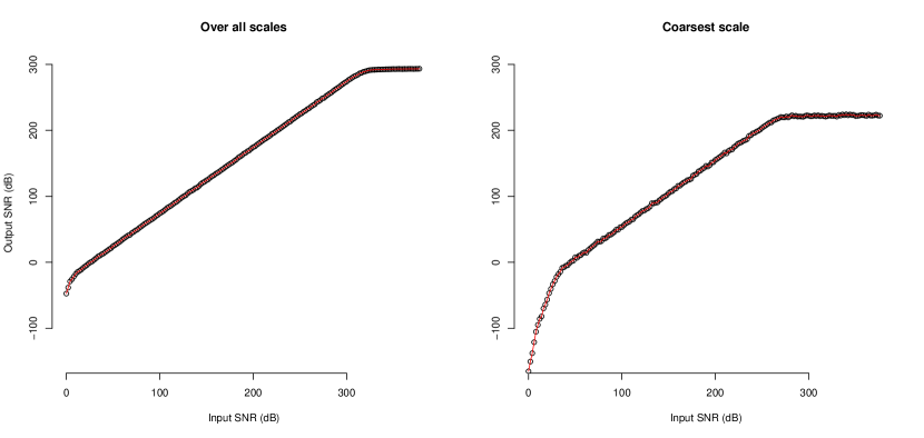
Figure 1: The relation between input and output SNR for the perturbed wavelet filter over all wavelet scales (2229superscript22superscript292^{2}-2^{9}, left panel) and for the coarse scale (22superscript222^{2}, right panel) within double machine precision.

To study truncation errors numerically, we generated a unit–power white noise time series (n=214𝑛superscript214n=2^{14}) (our results are qualitatively the same for different classes of time series), downsampled the time series by a factor of two using a FIR low pass filter of order N=30𝑁30N=30 (downsampling filter FIR1 Short et al. (2011)), and chose the difference of the low pass filter from the identity as our detail coefficients. Coefficients used in a typical estimation procedure depend on two integers: m𝑚m, the number of times the data is downsampled prior to estimation, and k𝑘k, the number of octaves used in the estimation. We used m=7𝑚7m=7 and k=6𝑘6k=6 in numerical analyses of the overall process for definiteness. The SNR for each scale was also studied individually. For error analysis, we perturbed the downsampling filter while systematically varying the standard deviation, λisubscript𝜆𝑖\lambda_{i}, of the noise ϵisubscriptitalic-ϵ𝑖\epsilon_{i} (equation 4) so that the input signal-to-noise ratio (SNRI)subscriptSNR𝐼\left(\mathrm{SNR}_{I}\right) ranged from 380 to 0 decibels (dB). For each input SNR, we chose 100 white noise time series, perturbed the downsampling filter, and investigated the effect of the input SNR for each time series to the output SNR of the filter given by

𝒪(SNRO)=10log10ijdij2ij(d~ijdij)2𝒪subscriptSNR𝑂10subscript10subscript𝑖𝑗superscriptsubscript𝑑𝑖𝑗2subscript𝑖𝑗superscriptsubscript~𝑑𝑖𝑗subscript𝑑𝑖𝑗2\mathcal{O}(\mathrm{SNR}_{O})=10\log_{10}\dfrac{\sum_{ij}d_{ij}^{2}}{\sum_{ij}(\tilde{d}_{ij}-d_{ij})^{2}} (15)

where dijsubscript𝑑𝑖𝑗d_{ij} is the ithsuperscript𝑖thi^{\mathrm{th}} detail coefficient obtained at level j𝑗j by subtracting the low pass filtered value from the coefficient prior to downsampling, and d~ijsubscript~𝑑𝑖𝑗\tilde{d}_{ij}is the same coefficient obtained from the perturbed filter (cf. equation 5).

The SNR of the output (SNROsubscriptSNR𝑂\mathrm{SNR}_{O}) was approximately linearly related to that of the input (SNRIsubscriptSNR𝐼\mathrm{SNR}_{I}) (Figure 1, left panel) with the equation

𝒪(SNRO)=25.8+0.994×𝒪(SNRI)𝒪subscriptSNRO25.80.994𝒪subscriptSNRI\mathcal{O}\left(\mathrm{SNR_{O}}\right)=-25.8+0.994\times\mathcal{O}\left(\mathrm{SNR_{I}}\right) (16)
Refer to caption
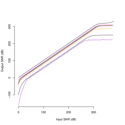
Figure 2: Degradation of output SNR as a function of scale. Progressively lower traces depict the relation for progressively coarser scales, from 213superscript2132^{13} to 22superscript222^{2}.

This relation shows that on average, a 104superscript10410^{-4} error in the estimated filter coefficients results in a 103superscript10310^{-3} error in the output. It should be noted, however, that this is a conservative estimate for the overall output error. In fact, stringent constraints may be necessary to attain sufficient accuracy at coarser scales because of the degradation of output SNR (Figure 2).
Refer to caption
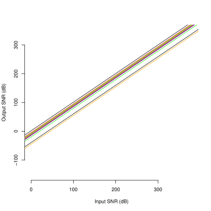
Figure 3: The linear relation between input and output SNR for scales 22superscript222^{2} to 213superscript2132^{13} in the 502705027050-270 dB input SNR range. Lower traces show the relation for coarser scales.
Table 1: Growing intercept of the relation between input and output SNR with coarser scales. See also Figure 3.
Scale (2nsuperscript2𝑛2^{n}) Intercept
2 -44.78
3 -39.86
4 -25.23
5 -14.59
6 -11.26
7 -9.87
8 -7.60
9 -4.61

Complete relation between 𝒪(SNRO)𝒪subscriptSNR𝑂\mathcal{O}(\mathrm{SNR}_{O}) and 𝒪(SNRI)𝒪subscriptSNR𝐼\mathcal{O}(\mathrm{SNR}_{I}) for the range of double machine precision (Figure 1, right panel) shows that between approximately 50 to 270 dB input SNR, output SNR is approximately a linear function (equation 16). In contrast, output SNR is flat when the input SNR is greater than 270 dB (where less than one bit of noise is added), and accelerates to -\infty from 0 dB when the input SNR is below 50 dB. Moreover, although the output SNR is linearly related to that of the input with a slope of 1 for all scales ranging from k=22𝑘superscript22k=2^{2} to k=29𝑘superscript29k=2^{9} within the range of 502705027050-270 dB input SNR (Figure 3; cf. equation 16), the intercept of this relation degrades at coarser scales (Table 1). Therefore, coarser scales are disproportionally affected. These results highlight that truncation errors in wavelet coefficients can quickly reach to unacceptable levels. For example, suppose that one requires the noise in the output of the coarse scale wavelet coefficients to be less than 111% of the output power. In this case, the noise power in the filter coefficients must be 100 dB, or the filter coefficients must produce errors less than approximately 5×1055superscript1055\times 10^{-5}.

Refer to caption
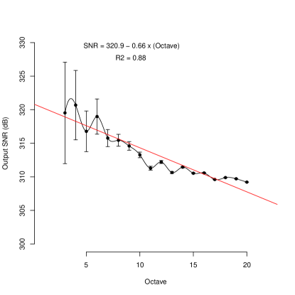
Figure 4: An error analysis for the FFT of size 28superscript282^{8}. The output SNR is over 300300300 dB, and the reduction in precision is about 0.850.850.85 for each additional octave. Vertical bars show 95% confidence intervals.

To put this error amplification in perspective, consider simple filtering via Fast Fourier Transform (FFT) of up to size 220superscript2202^{20}. In this case, SNR of the signal degrades only by about 20 dB from its maximal value of 306325306325306-325 dB (Figure 4). This relatively small loss indicates that in practice, memory would be exhausted before the truncation error becomes a problem. In contrast, the sub-band coding scheme reported here (thus, most wavelet filters) require a significant length convolution (N=30𝑁30N=30) at each stage of the calculation. Thus, whereas the FFT requires log2Nsubscript2𝑁\log_{2}N multiplications for each of the N𝑁N elements inverted, wavelet filtering and sub-band coding schemes can require 30log2Nsuperscript30subscript2𝑁30^{\log_{2}N} calculations. This difference can be significant at moderate input SNRs since repeated truncation errors may result in a catastrophic loss of precision.

IV Conclusion

Our results show that truncation error in the wavelet filter coefficients due to quantization and round-off may amplify due to the the multiplicative propagation, and can reach substantial levels. In cases where the relative error in the wavelet coefficients is too large, the wavelet tree (k)𝑘(k) grows too deep, or the wavelet filter (N)𝑁(N) is too long, this propagation of truncation errors may render the results unreliable especially at coarser scales. Note that although the sub-band analysis presented here is not identical to downsampling using Coiflets or Daubechies filters Daubechies (1982), small errors in the coefficients will still propagate in the latter case because the propagation depends strongly on the length of the filter applied prior to the downsampling. We expect errors with relatively large D15 (N=30𝑁30N=30 coefficient Daubechies) filter to be comparable to the case presented here.

References

  • Short et al. (2011) T. Short, U. Ligges, S. Schnackenberg, H.-W. Borchers, and S. Krey, Signal processing toolbox for R (2011).
  • Daubechies (1982) I. Daubechies, Ten Lectures on Wavelets (CBMS-NSF Regional Conference Series in Applied Mathematics), The Art of Computer Programming (SIAM: Society for Industrial and Applied Mathematics, 1982), 1st ed.