Bias in generation of random graphs

Abstract

We study the statistical properties of the generation of random graphs according the configuration model, where one assigns randomly degrees to nodes. This model is often used, e.g., for the scale-free degree distribution $\sim d^{\gamma}$. For the efficient variant, where non-feasible edges are rejected and the construction of a graph continues, there exists a bias, which we calculate explicitly for a small sample ensemble. We find that this bias does not disappear with growing system size. This becomes also visible, e.g., for scale-free graphs when measuring quantities like the graph diameter. Hence, the efficient generation of general scale-free graphs with a very broad distribution ($\gamma<2$) remains an open problem.

I Introduction

Networks have become a very valuable tool when analyzing complex systems like social communities, protein interactions, the Internet or the spread of diseases Watts (1999); Albert and Barabási (2002); Dorogovtsev and Mendes (2003); Newman (2003); Boccaletti et al. (2006); Newman and Barabási (2006). There are two basic approaches to analyze the creation, structure, and behavior of networks: One is to look at specific real-world networks and analyze as many parameters as possible, comparing them to other specific real-world networks. The second approach is to generalize form the given data and to find network ensembles which describe one or several real-world networks as close as possible. These ensembles are intended to be generated within computer simulations Hartmann (2009) and analyzed using statistical methods. Thus, one has to find methods for generating model networks exhibiting the desired features. These samples should have good statistical properties, which means that each realization of the graph should be created with a desired probability, often this the uniform ensemble. A generation method which fulfills this is called unbiased.

Well known ensembles are small-world networks Watts and Strogatz (1998); Watts (199) and scale-free networks, the latter exhibiting a power-law distribution with density

$$P(d)\sim d^{-\gamma}\quad(d>0)$$ (1)

for the degrees $d$, i.e., the number of neighbors of a node. Such a behavior for the degree distribution is often observed for real-world systems Redner (1998); Broder et al. (2000); Barabási et al. (2000); Jeong et al. (2000); Liljeros et al. (2001); Newman (2005). A very efficient method to generate random graphs is preferential attachment de Solla Price (1976); Barabási and Albert (1999); Dorogovtsev et al. (2000); Krapivsky and Redner (2001). For some networks, like citation networks, this is a very suitable model. Nevertheless, this does not allow to generate graphs with a very broad degree distribution $\gamma<2$. Also, the preferential attachment process does create certain correlations, in particular the obtained graphs are always connected. Hence, for general models which do not make any assumptions beyond the degree distributions, other methods have to be used.

A more general approach is to first draw a degree sequence from the desired degree distribution and in a second step to assign the edges randomly such that all simple graphs (without multiple connections or self-loops) which are feasible for this degree sequence are equiprobable Molloy and Reed (1995). Note that this generates labeled graphs, i.e., each node is distinguishable from the other nodes. This means, e.g., the (single) graph with degrees $d_{1}=2$, $d_{2}=1$, $d_{3}=1$ is different from the graph exhibiting $d_{1}=1$, $d_{2}=2$, $d_{3}=1$. A method which is frequently used for graphs with predefined degree sequences is the configuration model. Bender and Canfield Bender and Canfield (1978) and Bóllobas Bóllobas (1980) introduced the mathematical background in 1978–1980. A very efficient algorithm was described by Newman et al. Newman et al. (2001) in 2001. For each vertex with a given degree, stubs are created, which are the points where edges are emerging from the vertex. In a second step random pairs of stubs are connected until there are no stubs left. In order to be able to connect all stubs the total number of stubs must be even. For randomly drawn sets of stubs this can be archived by disregarding sets with an odd number of stubs and generating a new set. In the configuration model, however, it is possible that two stubs of the same vertex are connected creating a self loop, or two different vertices are connected with multiple edges. When statistically analyzing networks usually one considers simple graphs. Therefore self-loops and multiple edges have to be avoided when generating these graphs in a computer. There are several possibilities how to deal with this problem described in Britton et al. (2006).

One method (“refusal”), is to disregard all non-simple graphs and redo the algorithm until a simple graph is created. In other words, as soon as a self-loop or multiple edge is created all connections made so far have to be disregarded and the generation process is restarted. This procedure will generate all graphs with a given set of degrees with equal probability Britton et al. (2006). The disadvantage of this procedure is that many attempts may be needed to create a simple graph with this method,. This becomes quite annoying in particular for scale free graphs with a broad degree distribution ($\gamma<2$) where for a large number of nodes it becomes impossible to generate a single graph instance. For example, if one accepts for constructing a graph up to one CPU hour, for $\gamma=1$ only graphs with about $n=30$ nodes are feasible while for $\gamma=2$ one can go up to $n=300$.

In practice, in many publications a different approach (“repetition”) is used: Much fewer graphs are thrown away if, when encountering the generation of a forbidden edge, the connections made so far are kept and only the last connection is disregarded and a new pair of stubs is randomly drawn as explicitly mentioned by Milo et al. Milo et al. (2002) or later on by Catanzaro et al. Catanzaro et al. (2005). Apparently this approach is used in many applications, although sometimes no details are given how these conflicts during the graph generation are solved, like, e.g., in the original Ref. Newman et al. (2001). Nevertheless, the ensemble generated in this way exhibits a bias since now the sub-pairing probability depends on the graph generated so far. This was observed for one sample degree sequence of a very small multigraph by King King (2004). The existence of this bias leads to the question, whether this bias persists when going to larger, realistic graphs. In particular it could be that for measurable quantities, within error bars, the results of the true and the biased ensembles agree. We will show in this paper that indeed the bias persists when studying larger graphs, in particular it will be visible for a global graph property, the graph diameter.

The reminder of the paper is organized as follows: Next, in the second section, we introduce a simple restricted ensemble, which allows us to investigate its statistical properties as a function of the system size. We will understand for its smallest instance explicitly how the bias arises when repeating the creation of edges in case of forbidden edges. In the third section, we study this bias as a function of the system size, for a small range of sizes, where this is feasible. In the fourth section, we investigate the behavior of the graph diameter for ensembles of scale-free graphs. Finally, in the conclusions, we summarize our results and discuss other approaches like Markov chain Monte Carlo simulations Taylor (1982) or a recently proposed rejection-free method Genio et al. (2010) where the graphs carry additional weights.

II Example

Figure 1: Seven possible realizations of a graph with five vertices for the degrees $d_{1}=2,d_{2}=2,d_{3}=2,d_{4}=1,d_{5}=1$

In order to compare both variants of the configuration model, with edge repetition or without (i.e., refusal), we look at a simple example. Consider a graph with 5 vertices. For this example and for the examples in the subsequent section, we aim at graphs having roughly half of the nodes exhibiting degree 1 and half of the nodes degree 2. For our example here, the degree and therefore the number of stubs for each vertex is fixed as follows: $d_{1}=2,d_{2}=2,d_{3}=2,d_{4}=1,d_{5}=1$. Connecting all stubs can lead to two possible graph topologies as shown in figure 1. Either vertex 4 and 5 are connected and the resulting graph is split into two subgraphs ($A$), or the graph is a single line with a variable order of the vertices ($B$). For an unbiased sampling, each of the seven realizations of the graph should occur with the same probability. Since only one realization leads to the graph topology $A$ and 6 to the graph topology $B$, the ratio $\frac{p(A)}{p(B)}$ should be $\frac{1}{6}$. The process of building up the graph by connecting stubs using the approach where the process is restarted once an invalid edge is obtained (refusal) is illustrated in figure 2.

Figure 2: (color online) Generation of graph with five vertices having degrees $d_{1}=2,d_{2}=2,d_{3}=2$ (black circles), $d_{4}=1,d_{5}=1$ (open circles) with refusing non-simple graphs. Starting from the left, in each step two stubs are picked randomly and connected which can lead to several configurations, shown by pictographs. Configurations which are equivalent are summarized into one pictograph. For example, whether in the first step node 1 and 2, or node 1 and 3 are connected makes no difference. Possible transitions between configurations are indicated by lines. The transition probabilities to reach a certain configuration from the current one are indicated by rational numbers shown next to the lines. The probabilities to have reached a certain configuration are indicated by the rational numbers beneath the pictographs. Reaching a non-valid configuration is indicated by the “crossed out” graphs at the bottom of the different columns.

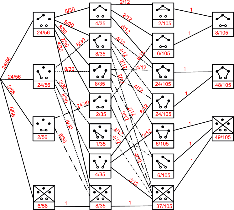
One starts (left Fig. 2) with a completely unconnected graph. In the first step one out of eight stubs is picked, the stub is removed from the pool and a second stub (out of the seven remaining ones) is picked at random. The associated vertices are connected. There are four different possible configurations after the first edge has been made. Three valid edges are: Two vertices of degree 2 are connected, a vertex with degree 2 is connected to a vertex with degree 1, or the two vertices with degree 1 are connected. A forbidden edge is attempted, if the first and the second stub belong to the same vertex, i.e., a self edge. This latter case is disregarded by restarting the graph-generation process. All probabilities shown in Fig. 2 can be easily calculated by hand. This leads finally to the probability $p$ for the different topologies. The probability to generate graph topology $A$ in one trial is $p(A)=\frac{8}{105}$, $p(B)=\frac{48}{105}$ and the probability to end up disregarding the graph is $p(C)=\frac{49}{105}$. Considering the valid topologies one finds a ratio of the two graph topologies of $p(A)/p(B)=1/6$ as expected. Hence, even for this small graph for only about 50% of the times the graph-generation process will lead to a valid graph while in the other case the process has to be restarted from an empty graph.

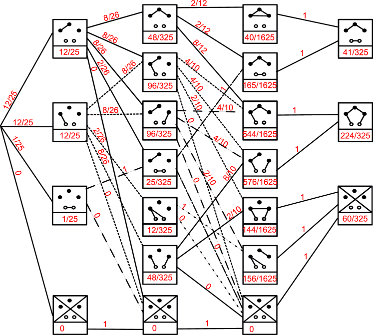
Fewer restarts are needed, if the second variant (repetition) is applied, i.e., if just the last pair of stubs leading to a forbidden edge is disregarded. This generation process is shown in figure 3. In each step the transition probability $p_{\rm trans}(i\to j)$ from one configuration $i$ to another $j$ is calculated in the following way: It contains the probability $p_{\rm direct}(i\to j)$ that the corresponding stubs are selected immediately. Nevertheless, since after an invalid choice the step is repeated, more terms contribute, e.g., the probability $p_{\rm error}(i)$ that first an invalid pair of stubs is selected times the probability $p_{\rm direct}(i\to j)$ that in the second try the corresponding stubs are selected. In the same way, also the probability contributes that two invalid tries are performed before a valid pair of subs is selected, and so on:

$$p_{\rm trans}(i\to j) = \sum_{n=0}^{\infty}p_{\rm direct}(i\to j)\left(p_{\rm error}(i)\right)^{n}$$ (2)

$$= \frac{p_{\rm direct}(i\to j)}{1-p_{\rm error}(i)}$$ (3)

By manually calculating these probabilities, on arrives at the process displayed in Fig. 3. Note that as long as there exists a valid edge which can be formed, this method does not have to restart the complete generation process. For this reason, the probability that one has to restart the full process is zero in early stages. There are however configurations towards the termination of the process which have only stubs left that lead to forbidden edges. In these few cases the generation process has to be restarted. The ratio of the two graph topologies is $p(A)/p(B)=\frac{41}{224}$ which is different from the correct ratio of $1/6=28/224$. The probability of forming a graph topology, where the graph splits into two subgraphs is too high, compared to the formation of a single line.

Figure 3: (color online) Generation of the same graph as shown in Fig. 2, see there for details, but now with repeated selection of pairs of stubs in case invalid edges are selected.

III Size-dependence

The number of vertices and the degrees in the example in previous section were chosen to be as simple as possible such that an effect can be observed. Nevertheless, one might wonder whether for larger graphs, the bias somehow decreases such that in the end it becomes unimportant. In order to investigate how this effect behaves for larger $n$, the two methods (refusal/repetition) are compared numerically by randomly generating a large number of graphs using a predetermined list of stubs and counting the number of generated instances for each graph realization. Again we aimed at graphs where roughly half of the nodes have degree 1 and the other half has degree 2. We considered graph sizes $n=6,8,10,12$. An even higher number of nodes is not feasible, because the number of possible graphs increases strongly. For $n=8$ and $n=12$ exactly half of the vertices have degree 1 and the other half has degree 2. For $n=6$ ($n=10$) two (four) vertices have degree 1 and four (six) vertices degree 2. This results in an even number of stubs in all cases. The number of generated graphs was chosen such that on average 10000 graphs were created per possible graph realization. The exact number of possible realizations (bins of the histogram) for each graph size $n$ can be found in table 1. The resulting histograms are shown in figure 4.

Figure 4: (color online) Histograms for number of generated graph realizations. The two approaches repetition (red x symbols) and refusal of non-simple graphs (black $+$ symbols) are compared for different graph sizes $n=6,8,10,12$.

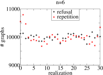
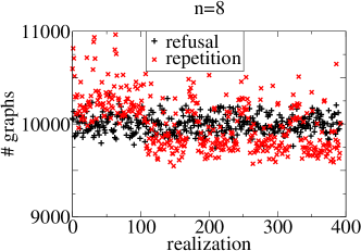
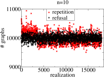
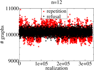
For all sizes shown in figure 4 each realization occurs, within statistical variation, with the same probability, if the entire graph is refused as soon as the first forbidden edge occurs. If just the forbidden edges are disregarded (repetition), some realizations appeared significantly more often than others. These deviations are especially prominent for large graph sizes. Hence, the bias of the repetition method does not disappear!

The make the statement also more quantitatively, we calculated p-values from a chi-squared test Hartmann (2009) for the sampled histograms assuming an equal distribution of realizations. The resulting p-values are shown in table 1. In addition to the p-values from 10000 sampled graphs per bin as used in the figures, also the resulting p-values for a smaller number of 1000 graphs per bin are shown.

n	# bins	1000/bin		10000/bin
		refusal	repetition	refusal	repetition
6	31	$0.75$	$2.8\cdot 10^{-3}$	$0.33$	$4.6\cdot 10^{-23}$
8	393	$0.52$	$8.5\cdot 10^{-19}$	$0.76$	$0.0$
10	18012	$0.15$	$4.1\cdot 10^{-142}$	$0.36$	$0.0$
12	332790	$0.91$	$0.0$	$1.0$	$0.0$

Table 1: The p-values obtained from a chi-squared test for the sampled histograms assuming an uniform distribution of realizations ($\leftrightarrow$ bins) for an average of 1000 and 10000 sampled graphs per bin.

The p-value for the refusal method varies between 0.15 and 1.00 for the different cases. This statically supports the result that all graph realizations are equiprobable, hence the ensemble is not biased. When using the method with repetition of edge creation the value is by several orders of magnitude smaller and decreases quickly for increasing graph size $n$. For a large number of samples per bin and/or large graphs, the p-value is even just 0 within the standard numerical accuracy. This clearly shows that the different graphs are not equiprobable.

Another way to analyze the statistics of the graph generation process is to find a measurable quantity that might differ on average when using different generation methods. Here, we considered the graph diameter , which is among all pairwise shortest path distances of a graph the longest one (omitting infinite distance if two nodes are not connected). For the sample graphs of Sec. II, one obtains an average diameter of $212/156\approx 3.79$ for the (unbiased) refusal approach, while for the repetition approach a much smaller value of $978/325\approx 3.01$ is obtained. For larger systems sizes the difference becomes smaller, but still measurable: The average diameter $d_{\max}$ and the standard error for $10^{7}$ randomly generated graphs of size $n=6,8,10,12$ with degrees as described above can be found in table 2. We state differences of the diameters normalized by the maximum standard error $\tilde{\sigma}$ given by

$$\Delta=(d_{\max}({\rm refusal})-d_{\max}({\rm repetition}))/\tilde{\sigma}\,.$$ (4)

The differences in diameter are now quite small but still statistically significant. Hence, studying measurable quantities might be a promising approach to investigate ensembles of even larger graphs, which we present in the next section.

$n$	$d_{\max}$ refusal	$d_{\max}$ repetition	$\Delta$
6	$2.4839\pm 0.0001$	$2.4771\pm 0.0001$	68
8	$2.4580\pm 0.0001$	$2.4570\pm 0.0001$	10
10	$2.8632\pm 0.0001$	$2.8628\pm 0.0001$	4
12	$2.7831\pm 0.0001$	$2.7843\pm 0.0001$	-12

Table 2: Mean diameter $d_{\max}$ and standard error for $10^{7}$ sampled graphs, for the refusal and repetition approaches, respectively, for different graph sizes $n$. The last column displays the normalized differences $\Delta$ of the diameters.

IV Diameter of scale-free graphs

To investigate, whether the bias present in the repetition approach is measurable for even larger graphs, we studied scale-free graphs where the node degrees are sampled from the distribution shown in Eq. 1. For $\gamma\leq 2$ the first moment of this distribution diverges in the thermodynamic limit. For $\gamma\leq 3$ the second moment diverges. This can lead to vertices with very high degrees. Figure 5 shows the mean diameter of scale-free graphs with exponents of $\gamma=2$, $3$, $4$ for 10000 generated graphs as a function of the number of vertices $n$. Here we also generated graphs where the maximum degree is cut off at $\sqrt{n}$. This cutoff was suggested by Catanzaro et al. Catanzaro et al. (2005) in order to remove degree correlations, which occur otherwise for $\gamma<3$. Also preventing very high degrees allows to generate larger graphs at low values of $\gamma$ using the refusal approach. Nevertheless, we only studied $\gamma\geq 2$, because otherwise the refusal method does not allow to study very large systems for all cases.

Figure 5: (color online) Average diameter $d_{\max}$ of scale-free graphs with exponents of $\gamma=2$, $3$ and $4$ for $10^{4}$ generated graphs as a function of the number of vertices $n$ using four different approaches. The error bars are smaller than the symbol size.

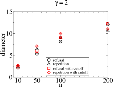
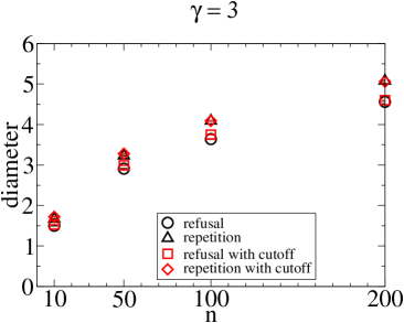
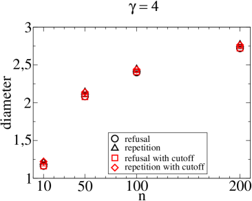
For $\gamma=2$ the diameters deviate depending on the method which is used for graph creation. The deviation increases for increasing system size. Including the cutoff increases the diameters for both generation approaches, but it does not reduce the difference between both generation methods. For $\gamma=3$, the differences between the different case become smaller. For $\gamma=4$ there is even very little difference in diameter for graphs generated with both methods. Introducing a cutoff for the highest degree does not change the diameter at all in this case, since high degrees are anyway very rare.

To study the differences between the unbiased refusal and the biased repetition approaches more quantitatively, we also calculated the normalized differences $\Delta$ (Eq. 4) between the average diameters, see Tan. 3. Clearly, even for large graphs, the error introduced by the bias of the repetition approach is quite significant.

$\Delta$	$n=10$	$n=50$	$n=100$	$n=200$
$\gamma=2$	-35	-37	-18	17
$\gamma=2$ cutoff	-34	-39	-18	21
$\gamma=3$	-28	-32	-23	-26
$\gamma=3$ cutoff	-32	-29	-17	-15
$\gamma=4$	-25	-15	-11	-8
$\gamma=4$ cutoff	-29	-15	-8	-7

Table 3: Normalized difference $\Delta$ between the average diameters for scale free graphs ($\gamma=2,3,4$), also when additionally introducing a degree cutoff at $\sqrt{n}$.

V Conclusions

We have studied the statistics of generating random (labeled, simple) undirected graphs with prescribed degree sequences using the configuration-model approach. The basic idea is to assign each node a number of stubs equal to its degree and then pair randomly selected stubs. This leads to an unbiased sample, i.e., the weight is uniform, if only valid simple graphs are kept and all others refused. In many cases, e.g., for scale-free graphs with a very broad tail, this is very inefficient. Hence, in the literature very often an approach is used where invalid edges are immediately rejected and instead the current stub-selection step is repeated. In this way much larger graphs can be generated, even for a very broad degree distribution. Nevertheless, this ensemble is biased, as can be seen from a very simple example of a graph with five nodes.

Our statistical analysis of related degree sequences for graphs sizes $n=6$, 8, 10, 12 shows that this bias does not disappear. Instead, by using a chi-squared test, we could show that the p-value decreases quickly such that it becomes zero within the numerical accuracy. Even worse, for measurable quantities like the diameter, the average estimates differ by many error bars, also for much larger sizes such as $n=200$. Hence, for a careful analysis of graphs, either with prescribed degree sequences or for an ensemble obtained by randomly drawing degree sequences, the configuration model with repetition does not work properly.

Recently, Del Genio et al. Genio et al. (2010) proposed a rejection-free approach which is based on restricting the sampling in each step to the set of edges such that for the remaining degree sequence there is still a simple undirected graph. The algorithm introduces a bias which is controlled by calculating weights which allow for correcting for this bias. Unfortunately, the distribution of weights exhibit a log-normal distribution. Hence, in each set of sampled graphs, there will be few samples which nevertheless carry a weight which is many orders of magnitude larger than the typical weight. In a sample study in Ref. Genio et al. (2010) for scale-free graphs with $\gamma=3$ and $n=100$, the largest sampled graph (among $10^{6}$ graphs) exhibited a weight which exceeded the typical weight by a factor of $10^{26}$. Hence, to calculate any measurable quantity, an extremely small number of graphs (usually one if the graphs are large) will contribute within a set of graphs generated by this approach. Note that the algorithm of Blitzstein and Diaconis Blitzstein and Diaconis (2006), which was proposed in 2006, suffers from the same problem. Therefore, it would be very useful to alter these approaches such that preferentially graphs with large weight are generated. Whether this is possible remains an open question in the moment.

Hence, to our knowledge, there is to data no practical approach which allows efficiently to sample graphs rejection-free of any given degree sequence without a bias. Hence, it appears that one still should use methods which are based on Markov-chain Monte Carlo methods, i.e. which start with any feasible graph and perform swaps of randomly selected edges Taylor (1982). Unfortunately, this approach creates correlations between subsequent graphs, hence one has to take additional effort to estimate mixing (decorrelation) times.

VI Acknowledgements

We thank Charo Del Genio for useful discussions. The simulations were performed at the HERO high-performance computing facility (supported by the DFG, INST 184/108-1 FUGG) at the University of Oldenburg.

References

- Watts (1999) D. J. Watts, Small Worlds (Princeton University Press, Princeton, NJ, 1999).
- Albert and Barabási (2002) R. Albert and A.-L. Barabási, Rev. Mod. Phys. 74, 47 (2002).
- Dorogovtsev and Mendes (2003) S. N. Dorogovtsev and J. F. F. Mendes, Evolution of Networks: From biological nets to the Internet and WWW (Oxford University Press, 2003).
- Newman (2003) M. E. J. Newman, SIAM Review 45, 167 (2003).
- Boccaletti et al. (2006) S. Boccaletti, V. Latora, Y. Moreno, M. Chavez, and D. U. Hwang, Phys. Rep. 424, 175 (2006).
- Newman and Barabási (2006) M. E. J. Newman and A. L. Barabási, The structure and dynamics of networks (Princeton University Press, Princeton, NJ, 2006).
- Hartmann (2009) A. K. Hartmann, Practical Guide to Computer Simulations (World Scientific, Singapore, 2009).
- Watts and Strogatz (1998) D. J. Watts and S. H. Strogatz, Nature 393, 440 (1998).
- Watts (199) D. J. Watts, Amer. J. Sociol. 105, 493 (199).
- Redner (1998) S. Redner, Eur. Phys. J. B 4, 131 (1998).
- Broder et al. (2000) A. Broder, R. Kumar, F. Maghoul, P. Raghavan, S. Rajagopalan, R. Stata, A. Tomkins, and J. Wiener, Computer Networks 33, 309 (2000).
- Barabási et al. (2000) A. L. Barabási, R. Albert, and H. Jeong, Physica A 281, 69 (2000).
- Jeong et al. (2000) H. Jeong, B. Tombor, R. Albert, Z. N. Oltvai, and A.-L. Barabási, Nature 407, 651 (2000).
- Liljeros et al. (2001) F. Liljeros, C. R. Edling, L. A. N. Amaral, H. E. Stanley, and Y. Aberg, Nature 411, 901 (2001).
- Newman (2005) M. E. J. Newman, Contemporaray Physics 43, 323 (2005).
- de Solla Price (1976) D. J. de Solla Price, J. Ameri. Soc. Inform. Sci. 27, 292 (1976).
- Barabási and Albert (1999) A. L. Barabási and R. Albert, Science 286, 509 (1999).
- Dorogovtsev et al. (2000) S. N. Dorogovtsev, J. Mendes, and A.N.Samukhin, Phys. Rev. Lett. 85, 4633 (2000).
- Krapivsky and Redner (2001) P. L. Krapivsky and S. Redner, Phys. Rev. E 63, 066123 (2001).
- Molloy and Reed (1995) M. Molloy and B. Reed, Rand. Struct. Algor. 6, 161 (1995).
- Bender and Canfield (1978) E. Bender and R. Canfield, J. of Comb. Theory A 24, 296307 (1978).
- Bóllobas (1980) B. Bóllobas, European J. Combin. 1, 311 (1980).
- Newman et al. (2001) M. E. J. Newman, S. H. Strogatz, and D. J. Watts, Phys. Rev. E 64, 026118 (2001).
- Britton et al. (2006) T. Britton, M. Deijfen, and A. Martin-Löf, Journal of Statistical Physics 124 No.6, 1377 (2006).
- Milo et al. (2002) R. Milo, S. Shen-Orr, S. Itzkowitz, D. Chklovskii, and U. Alon, Science 298, 824 (2002).
- Catanzaro et al. (2005) M. Catanzaro, M. Boguná, and R. Pastor-Satorras, Phys. Rev. E 71, 27103 (2005).
- King (2004) O. D. King, Phys. Rev. E 70, 058101 (2004).
- Taylor (1982) R. Taylor, SIAM Algor. Discr. Math. 3, 115 (1982).
- Genio et al. (2010) C. I. D. Genio, H. Kim, Z. Toroczkai, and K. Bassler, Plos One 5, e10012 (2010).
- Blitzstein and Diaconis (2006) J. Blitzstein and P. Diaconis (2006), unpublished.