Multifractal finite-size-scaling and universality at the Anderson transition
Abstract
We describe a new multifractal finite size scaling (MFSS) procedure and its application to the Anderson localization-delocalization transition. MFSS permits the simultaneous estimation of the critical parameters and the multifractal exponents. Simulations of system sizes up to and involving nearly independent wavefunctions have yielded unprecedented precision for the critical disorder and the critical exponent . We find that the multifractal exponents exhibit a previously predicted symmetry relation and we confirm the non-parabolic nature of their spectrum. We explain in detail the MFSS procedure first introduced in our Letter [Phys. Rev. Lett. 105, 046403 (2010)] and, in addition, we show how to take account of correlations in the simulation data. The MFSS procedure is applicable to any continuous phase transition exhibiting multifractal fluctuations in the vicinity of the critical point.
pacs:
71.30.+h,72.15.Rn,05.45.DfI Introduction
One of the most fascinating aspects of the Anderson localization-delocalization transition is the occurrence of multifractal fluctuations of the wavefunction intensity at the critical point.EveM08 ; MorKMG02 ; HasSWI08 ; FaeSPL09 While, strictly speaking, the fluctuations are truly multifractal only at the critical point, where the correlation length diverges, multifractal fluctuations nevertheless persist on either side of the transition on length scales less than the correlation length.Cuevas2007 The persistence of the fluctuations can be clearly seen in Fig. 1, where the wavefunction intensities for some typical critical, metallic and localized wavefunctions are plotted. In this paper we show how to exploit this persistence by combining multifractal analysis with finite size scaling to arrive at a very powerful method for the quantitative analysis of the Anderson transition, or any continuous phase transition that exhibits multifractal fluctuations: Multifractal Finite Size Scaling (MFSS).
Below we describe in detail the MFSS procedure and we demonstrate its potential by employing it to make a more comprehensive analysis of the Anderson transition in three dimensions than given in our Letter.RodVSR10 As we describe, the MFSS procedure permits the simultaneous estimation of the usual critical parameters, such as the location of the critical point and the critical exponent, and the multifractal exponents. Moreover, MFSS offers the opportunity to examine the consistency of the estimates of the critical parameters against the choice of multifractal exponent used in the scaling analysis.
The organization of the paper is as follows. In Section II, we describe briefly the Anderson model of a disordered systems and the numerical simulation of the Anderson transition. In Section III, we define the generalized multifractal exponents (GMFEs) used in MFSS, and derive the corresponding scaling laws. The relation between the GMFEs and the scaling properties of the probability density function (PDF) of wavefunction intensities is discussed in Section IV. In Section V we demonstrate the necessity of avoiding correlations in the wavefunctions. In Sections VI and VII we present results from standard and multifractal FSS, including estimates for the critical parameters and multifractal exponents. Finally, details of how to account for the inevitable correlations in different coarse grainings of the same simulation data, as well as how to check the stability of the scaling fits, are collected in the Appendices.
II The eigenstates of the Anderson model
We consider the three-dimensional (3D) Anderson Hamiltonian in site basis,
| (1) |
where site is the position of an electron in a cubic lattice of volume — where is measured in terms of the lattice constant —, denote nearest neighbors, periodic boundary conditions are assumed and are random on-site energies uniformly distributed in the interval . The Hamiltonian is diagonalized in the vicinity of the band centre for different degrees of disorder , close to the critical value where the localization-delocalization transition occurs. The eigenstates are numerically obtained using the Jadamilu library.SchBR06 ; BolN07 ; VasRR08
| 20 | 5138 (5006, 5374) |
|---|---|
| 30 | 5079 (5011, 5143) |
| 40 | 5168 (5012, 5351) |
| 50 | 5042 (5005, 5125) |
| 60 | 5027 (5009, 5082) |
| 70 | 5032 (5010, 5058) |
| 80 | 5028 (5013, 5048) |
| 90 | 5083 (5006, 5328) |
| 100 | 5024 (5020, 5041) |
| 110 | 4331 (4214, 4589) |
| 120 | 3103 (3000, 3757) |
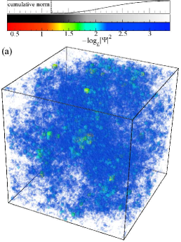
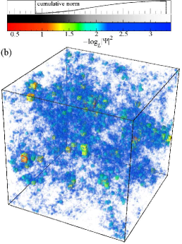
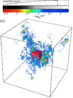
We have considered only a single eigenstate per sample (disorder realization), namely, the eigenstate with energy closest to . This is costly in terms of computing time, but as we shall show later, absolutely essential to avoid the strong correlations that exist between eigenstates of the same sample. System sizes range from to , and disorder values are in the interval . For each size and disorder combination, we have taken at least samples for , for a total of wavefunctions. The average number of states considered for each pair is indicated in Table 1. In Fig. 1 we show some wavefunctions for around the critical point.
III Scaling Laws for generalized multifractal exponents around the critical point
III.1 Multifractality at the critical point
It is known that the eigenstates of the 3D Anderson model (1) exhibit multifractal fluctuations at the critical point.Aok83 ; Jan94a ; EveM08 Here, we recapitulate briefly the basics of multifractal analysis.
To analyze the multifractal properties of wavefunctions in dimensions of a system of size , we coarse grain the wavefunction intensity on a scale . The system is partitioned into boxes of volume . A probability
| (2) |
is defined for each box . It is more convenient to work, not directly with the box probability , but with a related random variable , defined by
| (3) |
Here, is the ratio of the box size to the system size
| (4) |
Multifractality means that, if we count the number of boxes for which the value of the random variable falls in a given small interval , this number scales with as
| (5) |
in the limit that , i.e. that these boxes form a fractal with a fractal dimension that depends on . The set of all fractal dimensions is known as the multifractal spectrum.
Generalized inverse participation ratios (GIPR) or -moments are obtained by summing over the boxes
| (6) |
For later use, it is also convenient to define
| (7) |
As a consequence of multifractality it can be shown that at the critical point the GIPRs obey the scaling law
| (8) |
in the limit that . Here, the brackets denote an ensemble average. The mass exponents depend non-linearly on . They are conveniently expressed in terms of anomalous scaling exponents ,
| (9) |
The multifractal spectrum and the exponents are related via a Legendre transformation,
| (10) |
which defines singularity strengths and a singularity spectrum .
Multifractal exponents can also be defined from the scaling law corresponding to the geometric or typical average of the GIPRs
| (11) |
The relation between the typical and ensemble averaged multifractal exponents is now well understood, FosRL09 ; EveM08 and the multifractal properties of the 3D Anderson transition have been thoroughly studied using this standard formalism.SchG91 ; GruS95 ; MilRs97 ; VasRR08 ; RodVR08 ; RodVR08a
III.2 Multifractal behavior in the vicinity of the critical point
To extend multifractal analysis beyond the critical point we define a generalized mass exponent
| (12) |
Here, the tilde is used to emphasize that this equation applies throughout the critical region not just at the critical point. This generalized mass exponent becomes the usual mass exponent at the critical point in the limit .
Next we proceed to suggest a finite size scaling law for the GIPRs and from that derive a scaling law for these generalized mass exponents. Close to the transition, we may suppose that the GIPRs are determined by the ratios of the length scales and to the localization (correlation) length in the insulating (metallic) phase . This can be justified using renormalization group arguments,Car96 and is the basis for the scaling theory of localization.AbrALR79 ; LeeR85 This leads to the following scaling law for the GIPRsYakO98
| (13) |
At the critical point the correlation length has a power law divergence
| (14) |
described by a critical exponent . Thus, the scaling correctly reproduces the invariance of the GIPRs with exhibited by Eq. (8) at the critical point.
The scaling law for the GIPRs can be rearranged as follows to give a scaling law for the generalized mass exponents,
| (15) |
The function is related to the original . The factor has been explicitly included so that
| (16) |
The generalized anomalous scaling exponents
| (17) |
will then obey
| (18) |
By exact analogy with Eq. (10) we may define generalized singularity strengths
| (19) |
The scaling law for these quantities follows immediately from Eq. (15),
| (20) |
We may also define a generalized singularity spectrum
| (21) |
obeying a corresponding scaling law,
| (22) |
The scaling law for the GIPRs can be expressed in the entirely equivalent form
| (23) |
This remark applies equally well to the scaling laws for other quantities. Writing the scaling laws in this way immediately suggests a standard FSS analysis by fitting the disorder and system size dependence at fixed . As we show below this is indeed possible and works well. It does not, however, permit the estimation of the various multifractal exponents.
A much more exciting application of the above scaling laws (15)–(22) is to fit the variation with disorder, system size and box size. This allows not only the estimation of the usual critical parameters and but also the simultaneous determination of a multifractal exponent for a particular . Moreover, the use of different moments of the wavefunctions and different averages (ensemble, typical) provides a test of the stability of the estimates for the critical parameters, as these should be average- and -independent.
III.3 Averaging and the limit
| GMFE | Error estimation | Definition using the PDF |
|---|---|---|
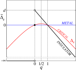
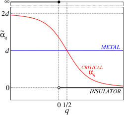
We emphasize that the generalized multifractal exponents (GMFEs) are equal to the corresponding scale invariant multifractal exponents only at the critical point in the limit .
Recalling the trivial scaling of and , we see that GMFEs and , independent of , , and . This is equivalent to .
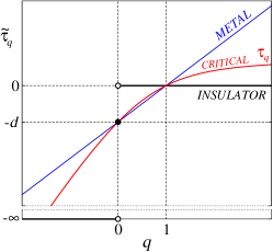
To understand better the behavior of the GMFEs as functions of , which is depicted schematically in Fig. 2, we discuss the expected behaviors in the thermodynamic limit in the metallic and insulating phases, and at the critical point.
In the metallic phase, for sufficiently large system size or sufficiently small disorder, the states are homogeneously extended and . It follows that , and for all .
In the insulating phase, for sufficiently large system sizes or large enough disorder, the wavefunctions approach an extremely localized state and . Then, for , , and . While for , the moments diverge, and . We emphasize that the insulating limit has been confirmed by analytical calculations for 3D exponentially localized states (with finite localization lengths).note-gmfelimit We note that the metallic and insulating limits can be reached either as or as for any fixed .
At the critical point, we recover the multifractal exponents as . These are known to obey a symmetry relation,MirFME06
| (24) |
or equivalently
| (25) |
This symmetry has been studied for Anderson transitions in different systems and dimensionality,MilSNE07 ; MilE07 ; EveMM08a ; ObuSFGL08 ; ObuSFGL07 ; FyoOR09 ; RodVR08 and has also been experimentally measured.FaeSPL09 The corresponding limits for can be obtained following similar reasonings and calculations.note-gmfelimit
IV Scaling for the PDF of wavefunction intensities around the critical point
It is also possible, and indeed, sometimes more convenient, to work directly with the probability density function (PDF) of .RodVR09 At the critical point the distribution is multifractal
| (26) |
and exhibits scale invariance, provided that is held fixed. Equation (26) can be used to estimate the multifractal spectrum directly from numerically calculated histograms of values.RodVR09 When we broaden attention to the critical regime, we find that, when is sufficiently small, we may approximate the PDF using the generalized multifractal spectrum (21)
| (27) |
This relation could be the basis for an alternative definition of the generalized singularity spectrum from the PDF. While there will be quantitative differences with (21) we would expect the results of scaling analysis to be unchanged.
The GMFEs can be obtained from the PDF. We consider as an example. Setting in Eq. (19) we have
| (28) |
The result of averaging is the same for all boxes, so
| (29) |
Thus corresponds to the mean value of the PDF. Expressions for general are given in Table 2.
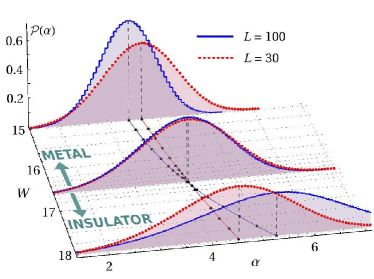
The scaling of with system size for fixed in the vicinity of the transition is shown in Fig. 3. This figure shows clearly that the scaling of the distribution of wavefunction intensities, or the distribution of a related quantity such as the local density of states (LDOS), could be used to characterize the Anderson transition.MirF94 Indeed, in Ref. RodVSR10, the critical parameters were successfully estimated from a scaling analysis of the system size and disorder dependence of the maximum of the PDF of at fixed . A similar procedure might be applied to experimental LDOS data obtained using STM techniques,HasSWI08 ; RicRMZ10 ; MorKMG02 ; KraCWC10 ; MilKRR10 or by direct imaging of ultracold atom systems.BilJZB08 ; RoaDFF08
V Remarks on correlations amongst wavefunctions
In exact diagonalization studies of disordered systems, it is common practice to average over eigenstates located within a small energy window. This is because the initialization and diagonalization of very large matrices is computationally demanding. Time can be saved by generating several eigenstates for the same sample. There is, however, a price to be paid. Eigenstates of the same sample are correlated, since they are solutions of the Schrödinger equation with the same potential. We have found that these correlations distort the statistical analysis. In particular, the error estimation becomes unreliable and the precision of critical parameters is overestimated, i.e. the error bars are erroneously small.
To quantify the correlations amongst wavefunctions from the same sample, we have studied the average correlation between two eigenstates with energies , , close to , such that . The correlation is defined as,
| (30) |
Here, is the -th power of the box probability Eq. (2) for the eigenstate with energy , and the prime indicates the same quantity calculated for the eigenstate with energy . The covariance is calculated using (47), where the sum is over boxes. The covariance is normalized to the product of the standard deviations, where again the sum is over boxes. The correlation can thus be calculated for two eigenfunctions from the sample, or two eigenfunctions from a pair of samples. A further ensemble average over samples, or pairs of samples, as appropriate, was taken to arrive at Fig. 4. On the left is the correlation obtained using pairs of eigenstates of the same sample. On the right is the correlation obtained using eigenstates of two different samples. A maximum correlation (anticorrelation) corresponds to , whereas statistical independence implies a vanishing . The correlation is shown as a function of the moment , for different degrees of coarse-graining and for three values of the disorder . (Note that, in the limit , the numerator and the denominator in (30) both go to zero. The finite solution of this indetermination is not necessarily unity, as one may naively expect.) Near the critical point, the correlation between eigenstates of the same sample is high, while for eigenstates of different samples correlation is, as expected, absent. We conclude that it is not safe to include in the MFSS analysis more than one state from a given sample, as these correlations render the subsequent statistical analysis unreliable.
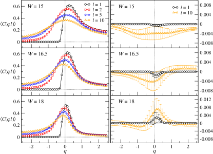
On the left of Fig. 4 we observe how the correlation varies with . For large positive , large wavefunction amplitudes dominate the -th moment of the box probability, while for large negative small amplitudes dominate. In both cases the correlation is reduced. We think that this occurs because only a small number of boxes contribute significantly to the extreme values of the distribution. We have checked that the overall shape of the correlations in the insulating regime agrees with calculations for 1D exponentially localized states. Another feature is that for negative correlations are absent for box size but are restored when the wavefunction is coarse-grained. This may indicate that very small wavefunction amplitudes are affected by random noise, which averages away when the wavefunction is coarse-grained. We have verified that similar behavior occurs for wavefunctions calculated using other numerical libraries, e.g. LAPACK.AndBBB87 We strongly recommend the use of coarse-graining to evaluate negative moments, even for 1-D models, such as power-law random banded matricesMirFME06 and others.FyoOR09
We emphasize that in this work — with the exception of the data on the left of Fig. 4 — we have used only one eigenfunction per sample.
VI Single-parameter scaling at fixed
We study first the scaling of the GMFEs , , , at fixed .note-scalinglaw This simplifies the scaling laws (18) and (20), which become one parameter functions,
| (31) |
where denotes any of the above mentioned exponents. Since is fixed, the multifractal exponents cannot be estimated, as they merge with the zero-th order term in the expansion of the scaling functions and (see Eqs. (18) and (20)). Nevertheless the critical disorder and the critical exponent can be estimated. We demonstrate the consistency of the estimates of these parameters for different values, and their independence on the type of average (typical or ensemble) considered.
VI.1 Expansion in relevant and irrelevant scaling variables
In order to fit data for the GMFEs, we follow the standard procedure of Ref. SleO99a, and include two kinds of corrections to scaling, (i) nonlinearities of the dependence of the scaling variables, and (ii) an irrelevant scaling variable that accounts for a shift with of the apparent critical disorder at which the curves cross. After expanding to first order in the irrelevant scaling variable, the scaling functions take the form
| (32) |
Here, and are the relevant and irrelevant scaling variables, respectively. The irrelevant component is expected to vanish for large , so . Both the scaling functions are Taylor-expanded
| (33) |
The scaling variables are expanded in terms of up to order and , respectively,
| (34) |
The fitting function is characterized by the expansion orders . The total number of free parameters to be determined in the fit is (including , and ).
The localization (correlation) length, up to a constant of proportionality, is . After subtraction of corrections to scaling
| (35) |
and the data for the GMFEs should fall on the single-parameter curves
| (36) |
VI.2 Numerical procedure at fixed
When performing FSS, the aim is to identify a stable expansion of the scaling function that fits the numerical data. The best fit is found by minimizing the statistic over the parameter space. The validity of the fit is decided by the -value or goodness-of-fit. We take as the threshold for an acceptable fit. As a rule of thumb the expansion orders are kept as low as possible while giving acceptable and stable fits. Once a stable fit has been found, the precision of the estimates of the critical parameters is estimated by Monte Carlo simulation, i.e. by fitting a large set of synthetic data sets generated by adding appropriately scaled random normal errors to an ideal data set generated from the best-fit model. A detailed description of the FSS procedure, with some examples, is given in Appendix A.
We performed a detailed FSS analysis for and for both ensemble and typical averages for different values of at a fixed value of , i.e. the box-size is always . The GMFEs were obtained for system-sizes ranging between and and for values of the disorder . The average number of independent wavefunctions involved in the calculation for each , is indicated in Table 1.
VI.3 Results for
| Average | ||||||||||
|---|---|---|---|---|---|---|---|---|---|---|
| ENS | 10 | 181 | 0.39 | 3 1 2 0 | ||||||
| TYP | 10 | 177 | 0.49 | 3 1 2 0 | ||||||
| ENS | 11 | 181 | 0.38 | 4 1 2 0 | ||||||
| TYP | 10 | 177 | 0.49 | 3 1 2 0 | ||||||
| ENS | 11 | 180 | 0.40 | 4 1 2 0 | ||||||
| TYP | 10 | 178 | 0.47 | 3 1 2 0 | ||||||
| ENS | 11 | 176 | 0.49 | 3 2 2 0 | ||||||
| TYP | 11 | 173 | 0.56 | 4 1 2 0 | ||||||
| ENS | 12 | 168 | 0.63 | 5 1 2 0 | ||||||
| TYP | 12 | 171 | 0.58 | 5 1 2 0 | ||||||
| ENS | 12 | 167 | 0.65 | 5 1 2 0 | ||||||
| TYP | 12 | 182 | 0.33 | 4 1 3 0 | ||||||
| ENS | 11 | 174 | 0.53 | 4 1 2 0 | ||||||
| TYP | 11 | 178 | 0.45 | 4 1 2 0 | ||||||
| ENS | 11 | 172 | 0.56 | 4 1 2 0 | ||||||
| TYP | 11 | 167 | 0.64 | 5 0 2 0 | ||||||
| ENS | 11 | 175 | 0.51 | 4 1 2 0 | ||||||
| TYP | 11 | 168 | 0.65 | 4 0 3 0 | ||||||
| ENS | 11 | 174 | 0.52 | 4 1 2 0 | ||||||
| TYP | 11 | 170 | 0.61 | 4 1 2 0 | ||||||
| ENS | 12 | 166 | 0.67 | 4 1 3 0 | ||||||
| TYP | 12 | 168 | 0.64 | 4 2 2 0 | ||||||
| ENS | 10 | 179 | 0.45 | 3 1 2 0 | ||||||
| TYP | 10 | 178 | 0.47 | 3 1 2 0 | ||||||
| ENS | 10 | 182 | 0.38 | 3 1 2 0 | ||||||
| TYP | 10 | 175 | 0.52 | 3 1 2 0 | ||||||
| ENS | 10 | 184 | 0.34 | 3 1 2 0 | ||||||
| TYP | 10 | 176 | 0.50 | 3 1 2 0 | ||||||
| ENS | 11 | 179 | 0.43 | 3 2 2 0 | ||||||
| TYP | 10 | 179 | 0.45 | 3 1 2 0 | ||||||
| ENS/TYP | 10 | 175 | 0.53 | 3 1 2 0 | ||||||
| ENS | 12 | 178 | 0.43 | 4 1 3 0 | ||||||
| TYP | 12 | 187 | 0.25 | 4 1 3 0 | ||||||
| ENS | 13 | 168 | 0.62 | 4 2 3 0 | ||||||
| TYP | 14 | 168 | 0.59 | 5 2 3 0 | ||||||
| ENS/TYP | 13 | 168 | 0.61 | 4 3 2 0 | ||||||
| ENS | 11 | 176 | 0.48 | 4 1 2 0 | ||||||
| TYP | 11 | 171 | 0.59 | 4 1 2 0 | ||||||
| ENS | 11 | 183 | 0.35 | 5 1 1 0 | ||||||
| TYP | 11 | 194 | 0.17 | 5 1 1 0 | ||||||
| ENS | 10 | 175 | 0.54 | 4 1 1 0 | ||||||
| TYP | 10 | 172 | 0.58 | 3 2 1 0 | ||||||
| ENS | 9 | 169 | 0.68 | 4 0 1 0 | ||||||
| TYP | 10 | 187 | 0.28 | 4 1 1 0 |
The details of the fits are listed in Table 3.note-fits In Fig. 5 we plot the estimates of , , and , along with their confidence intervals, as functions of .
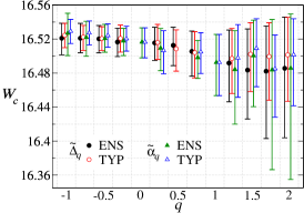
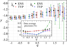
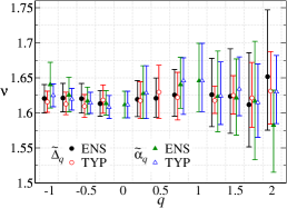
The estimates of the critical disorder, critical exponent and irrelevant exponent, both for different values of the power and the type of average considered, are mutually consistent. The values are also consistent with previous estimates obtained using transfer-matrix methods.SleO99a ; MilRSU00 ; SleOK00 The value of the irrelevant exponent is not directly comparable with previous transfer matrix studies since it is not clear that the dominant irrelevant correction should be the same for wavefunction intensity data.
In Fig. 5 there is a clear tendency for the error bars to increase for . This occurs because the average precision of the data (see the inset in Fig. 5) degrades quickly for , especially for the ensemble average. In general, for the same number of states, the precision is better when typical average is considered. Also, for , the precision of the data for is significantly better than that for , although this doesn’t translate into smaller uncertainties for the critical parameters.
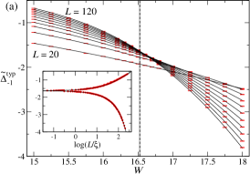
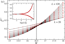
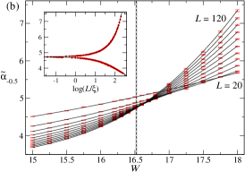
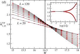
In Fig. 6 we show some examples of the calculated GMFEs together with the corresponding best fits. The FSS plots can be understood from the phase diagrams for the GMFEs discussed in Section III and depicted in Fig. 2. The GMFEs for () tend towards the metallic (insulating) limit as , which is located above or below the corresponding critical value depending on . We recall that, at fixed , the value of the GMFE at the crossing point does not correspond to the scale invariant multifractal exponent, which is recovered only as .
VI.4 The range
For , the expected critical value of is not located between the values of the metallic and insulating limits (see Fig. 2). This anomalous behavior makes a reliable FSS analysis in this interval of very difficult.
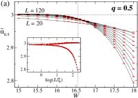
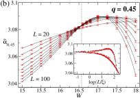
For the values in the metallic limit and at the critical point are expected to be the same (), while the value in the insulating limit is expected to be zero. As shown in Fig. 7(a), for and the data are almost independent of both and . While, for , the dependence on is very strong, as the data tend to the insulating limit. This behavior cannot be reliably described by a power series expansion.
For the value of at the critical point is now expected to be larger than the values in both the metallic and insulating limits. Data for is shown in Fig. 7(b). Very close to the critical point, a standard scaling behavior with opposite dependence at each side of the transition is visible. However, for larger disorder, the dependence is again reversed so as to approach the value in the insulating limit. We wish to emphasize that this is not a numerical artefact. Rather, analytical calculations for 3D exponentially localized states confirm the behavior.
VII Multifractal FSS
We now consider the scaling behavior of the GMFEs as function not only of disorder and system size but in addition the box-size using scaling laws (18) and (20). This permits the simultaneous estimation of the multifractal exponents and the critical parameters , , . This is a major advance over traditional multifractal analysis, where the position of the critical point must be estimated in a separate FSS analysis before the multifractal analysis.
VII.1 Fitting of correlated data
Different coarse-grainings for the same disorder and system size use the same set of eigenstates, which induces correlations among the estimates of GMFEs for different and the same and . These correlations must be properly taken into account in MFSS. To do so we generalize the definition of in the numerical minimization by including the full covariance matrix for the GMFEs. We describe the calculation of the covariance matrix and the -minimization procedure for correlated data in Appendices B and C.
VII.2 Expansion of scaling functions
In MFSS, the scaling functions are functions of two independent variables and . While these variables are independent because the system size and the box size vary independently, they involve the same scaling variable and renormalize in the same way. In addition, we need to allow for non-linear dependence in and for irrelevant scaling variables. We have found that the most important irrelevant contribution is due to the box-size . Therefore, we use the expansion
| (37) |
and similarly for . Here, and are the relevant and irrelevant scaling variables, with and the corresponding exponents. Note that we expand to second order in the irrelevant variable. We find that this is necessary to fit the data reliably. The functions are expanded,
| (38) |
for , as are the fields as described in Eq. (34). The expansion of the scaling function is then characterized by the indices . The number of free parameters is given by
| (39) |
After subtraction of irrelevant corrections we have
| (40) |
and the numerical data should fall on a common surface rather than a common curve as in standard FSS.
VII.3 Results
We have carried out the MFSS analysis on the ensemble averaged GMFEs for different , and for . The estimates of the critical parameters and the multifractal exponents, together with full details of the fits, are included in Table 4.
We have considered different ranges of data for different trying to maximize the number of points that we could fit in a stable manner, while keeping the value of . The minimum values of occurring in our data sets are () for and () for . Because of the need for coarse-graining for negative , as discussed in Section II, we exclude all data for .
| ( for ) | (prec.) | Expansion | |||||||
|---|---|---|---|---|---|---|---|---|---|
| 25 | 667 | 0.36 | 3 2 1 1 1 1 2 0 | ||||||
| 25 | 667 | 0.36 | 3 2 1 1 1 1 2 0 | ||||||
| 25 | 460 | 0.59 | 3 2 1 1 1 1 2 0 | ||||||
| 26 | 379 | 0.76 | 4 2 1 1 0 1 2 0 | ||||||
| 27 | 473 | 0.40 | 3 2 2 1 1 1 2 0 | ||||||
| 27 | 429 | 0.14 | 4 2 1 1 0 1 3 0 | ||||||
| 29 | 500 | 0.12 | 4 2 2 1 0 1 3 0 | ||||||
| 27 | 530 | 0.34 | 4 2 1 1 0 1 3 0 | ||||||
| 27 | 597 | 0.35 | 4 2 1 1 0 1 3 0 | ||||||
| 23 | 515 | 0.57 | 4 1 1 1 1 1 2 0 | ||||||
| 23 | 531 | 0.37 | 4 1 1 1 1 1 2 0 | ||||||
| 23 | 549 | 0.20 | 3 1 2 1 1 1 2 0 | ||||||
| 19 | 566 | 0.11 | 3 1 1 1 0 1 2 0 |
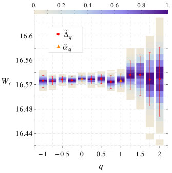
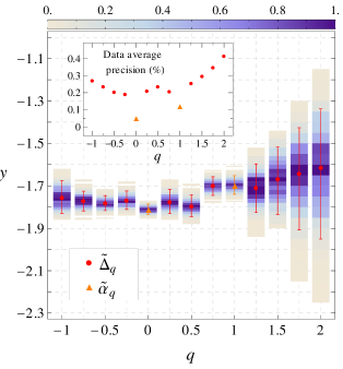
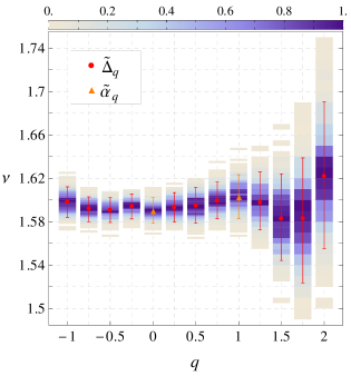
The best-fit estimates for , and as functions of are shown in Fig. 8. The consistency of the estimates of the critical parameters for different is remarkable. Compared with the FSS at fixed of Section VI, the estimate of the irrelevant exponent is more stable. As increases, the uncertainty for the estimates of , and grow. This is partly due to the loss of precision in the data for high (see the inset in Fig. 8), but this does not fully explain the large difference in the uncertainty between sets with similar precisions, for example and . We believe that the difference is caused by the amplitude of the irrelevant component in the data, which is larger for . (We have confirmed this by examining the dependence of the coefficient in the expansion (37).) If the amplitude of the irrelevant shift in the data is small, the estimation of the irrelevant exponent becomes very ambiguous. This in turn leads to an increase in the uncertainties of all the other parameters. The best precision is achieved for (). From the MFSS analysis of this GMFE we find
| (41) |
and
| (42) |
where the error limits correspond to confidence intervals.
VII.4 Scaling surfaces
In Fig. 9 we show the best fits and the corresponding scaling surfaces for and . The upper plots display the GMFEs and cross-sections of the global fit displayed at the different values occurring in the data set. The bottom plots show the scaling functions in terms of the two variables and . (The visualization of the scaling functions is improved when is chosen instead of as the second variable.) The scale invariant multifractal exponents correspond to the asymptotic value at the critical point as . This is highlighted in the insets of Fig. 9(c,d), where the behavior of the scaling function at criticality — when the sheets of extended and localized phases meet — is shown versus .
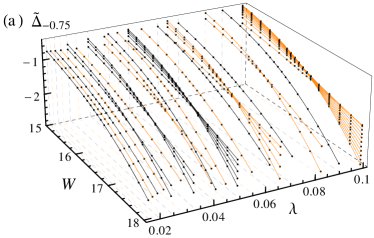
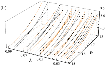
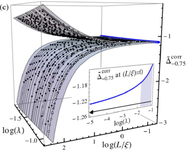
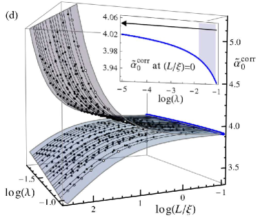
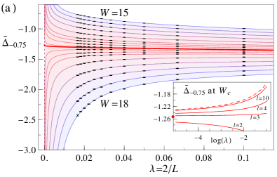
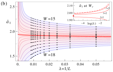
The transition can also be visualized as shown in Fig. 10 where we display a cross-section at fixed box-size of the data and the fit for and . This provides an alternative way to monitor the Anderson transition.WafPL99 ; AniKPF07 ; KraS10 We see the flow with increasing (decreasing ) towards the metallic or insulating limits depending on the disorder , and at the critical point the convergence to the multifractal exponent. At the critical point, the scaling law (37) reduces to
| (43) |
From this we find that this convergence differs for different . This is illustrated in the insets of Fig. 10.
VII.5 The multifractal spectrum
Previous work by some of the authors, using standard multifractal analysis at , suggested that the symmetry relation (24) for holds for the 3D Anderson model.VasRR08 ; RodVR08 ; RodVR09 Our improved analysis given here confirms this at . As shown in Fig. 11, the exponents satisfy the symmetry relation for the range of values considered.
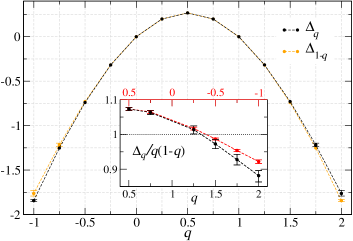
The symmetry relation (25) for , is also satisfied by our estimates and . A more careful analysis in terms of the reduced exponents reveals a slight violation of the symmetry beyond . We suspect that this reflects minor limitations in our extrapolation, rather than a genuine violation of the symmetry relation. (Particulary for where the range of is more restricted because of the absence of data for .) We note that the validity of the symmetry relation for the whole -range depends on the absence of termination points for the ensemble average multifractal spectrum,EveM08 which is still an open question for the 3D Anderson transition.RodVR09
Our data in Fig. 11 (inset) clearly show that the multifractal spectrum is not parabolic, i.e. that the reduced exponents depend on . This is in agreement with previous results at the 3D Anderson transition, where non-parabolicity has been directly observed in ,RodVR08 and in the non-Gaussian nature of the PDF, .RodVR09 ; HuaW10 A non-parabolic multifractal spectrum implies that the distribution of wavefunction intensities at the transition, and consequently also of the LDOS, is not a log-normal distribution, in contrast to recent claims.SchSBF10
VIII Conclusions
We have shown how to exploit the persistence of multifractal fluctuations away from the critical point on scales below the correlation length to perform a multifractal finite size scaling analysis. We demonstrated the potential of this approach by applying it to the Anderson localization-delocalization transition in the 3D Anderson model. We validated our proposed scaling laws for the generalized multifractal exponents and we estimated the critical disorder at the band center and the critical exponent describing the divergence of the localisation length . A remarkable consistency of these estimated critical parameters for different averages (ensemble and typical) and different generalized multifractal exponents (different ) was seen. We also found that the multifractal spectrum exhibits the predicted symmetry and confirmed its non-parabolic nature.
Recently, the value of for the Anderson transition has been estimated for a variety of systems, including disordered phonons PinR11 , electrons in non-conventional lattices EilFR08 or with topological disorder, KriA11 a disordered Lenard-Jones fluid, HuaW09 and cold-atom quantum kicked-rotors, ChaLGD08 ; LemCSG09 finding agreement with our results. The universality of the critical exponent for the Anderson transition is, therefore, well established and a value for is widely accepted by the community.
In our approach, scaling versus system size yields the critical exponent, while scaling versus box size yields the multifractal exponents. Thus, these exponents do not appear to be intrinsically related. Nevertheless, such a connection has been suggested by Kramer Kra93 and Janssen,Jan94a who discussed a lower bound for in terms of the multifractal exponents, namely
| (44) |
From our estimate of , the confidence interval for is . Remarkably, all our estimates for fall within this interval. Although this bound has not been widely discussed in the literature, we find the agreement intriguing.
Multifractal fluctuations have been observed in the local density of states near the metal-insulator transition in semiconductorsMorKMG02 ; HasSWI08 ; RicRMZ10 and in the intensity fluctuations of ultrasound near the Anderson transition in a random elastic network.HuSPS08 ; FaeSPL09 We believe that multifractal finite size scaling as demonstrated here has potential in the quantitative analysis of this sort of experimental data.KraCWC10 ; MilKRR10 ; BilJZB08 ; RoaDFF08 ; ChaLGD08 ; LemCSG09 ; LemLDS10
Acknowledgements.
The authors gratefully acknowledge EPSRC (EP/F32323/1, EP/C007042/1, EP/D065135/1) for financial support. A.R. acknowledges financial support from the Spanish government (FIS2009-07880).Appendix A Fitting procedure
A.1 Table of fits.
The first step is to generate a table of fits by varying the expansion indices of the model over a reasonable range of values. Since the number of combinations of the indices increases exponentially, we impose sensible restrictions. Let us consider, for example, the single-parameter FSS of Section VI, where the expansion (32) is characterized by the indices . We expect the irrelevant components to be less important than the relevant part of the scaling function. Therefore we impose the restriction and . For the single-parameter FSS we generate tables for each containing usually a few hundred index-combinations. For the MFSS of Section VII we generate initial tables of index-combinations for each and for different sets of data.
We decide whether or not a fit is acceptable based on the goodness-of-fit or -value. This is the probability that for degrees of freedom we would observe a value of larger than the one obtained for the best fit. To calculate this probability we use the approximation
| (45) |
Here, is the Euler gamma function, is the upper incomplete gamma function, and denotes the number of degrees of freedom in the model, i.e. the number of data minus the number of free parameters in the fit. We use as a criterion for an acceptable fit.
After excluding unacceptable fits we order the table according to the number of free parameters.
A.2 Stability of fits.
A good fit must not only give an acceptable value, it must also be stable. By stable we mean that the estimates of the fit parameters, and specially of the critical parameters, must not change significantly when the expansion orders are increased. In order to check the stability of a particular expansion, for example in fixed- FSS, we consider all expansions where each index is separately increased by , and also the case where all indices are increased by at the same time. If the critical parameters from all these fits lie within the uncertainty interval obtained for the estimates of the initial expansion, then we regard that fit as stable. The search for a stable fit proceeds by considering acceptable fits from the initial table in increasing order with the number of free parameters. As a general rule we try to find the simplest stable fit. We give examples of this procedure in Tables 5 and 6. While the criterion for a stable fit can certainly be debated we think that our criterion is sensible and helps avoid the ambiguity that may arise from an arbitrary choice of a particular fit with an acceptable value.
| 3 1 2 0 | 10 | 178 | 0.47 | 16.521 | 1.726 | 1.610 |
| - 3 1 2 1 - | 11 | 172 | 0.58 | 16.512 | 1.701 | 1.602 |
| - 3 1 3 0 - | 11 | 174 | 0.53 | 16.521 | 1.718 | 1.609 |
| 3 1 3 1 | 12 | 171 | 0.57 | 16.516 | 1.691 | 1.600 |
| - 3 2 2 0 - | 11 | 172 | 0.58 | 16.520 | 1.712 | 1.613 |
| 3 2 2 1 | 12 | 172 | 0.56 | 16.519 | 1.702 | 1.603 |
| 3 2 3 0 | 12 | 171 | 0.57 | 16.517 | 1.704 | 1.618 |
| 3 2 3 1 | 13 | 171 | 0.55 | 16.516 | 1.697 | 1.610 |
| - 4 1 2 0 - | 11 | 173 | 0.55 | 16.523 | 1.723 | 1.619 |
| 4 1 2 1 | 12 | 172 | 0.56 | 16.519 | 1.704 | 1.604 |
| 4 1 3 0 | 12 | 173 | 0.53 | 16.523 | 1.722 | 1.618 |
| 4 1 3 1 | 13 | 171 | 0.55 | 16.517 | 1.696 | 1.605 |
| 4 2 2 0 | 12 | 172 | 0.56 | 16.521 | 1.714 | 1.615 |
| 4 2 2 1 | 13 | 172 | 0.54 | 16.521 | 1.716 | 1.618 |
| 4 2 3 0 | 13 | 170 | 0.56 | 16.519 | 1.709 | 1.624 |
| - 4 2 3 1 - | 14 | 170 | 0.54 | 16.518 | 1.704 | 1.619 |
| Expansion | |||||||
|---|---|---|---|---|---|---|---|
| 3 2 2 1 1 1 2 0 | 27 | 473 | 0.40 | 16.530 | 1.811 | 4.048 | 1.590 |
| 4 2 2 1 1 1 2 0 | 30 | 466 | 0.46 | 16.531 | 1.811 | 4.048 | 1.593 |
| 3 3 2 1 1 1 2 0 | 31 | 467 | 0.43 | 16.530 | 1.810 | 4.048 | 1.592 |
| 3 2 3 1 1 1 2 0 | 29 | 466 | 0.46 | 16.531 | 1.813 | 4.048 | 1.593 |
| 3 2 2 2 1 1 2 0 | 30 | 466 | 0.46 | 16.532 | 1.813 | 4.048 | 1.591 |
| 3 2 2 1 2 1 2 0 | 29 | 472 | 0.39 | 16.530 | 1.806 | 4.047 | 1.591 |
| 3 2 2 1 1 2 2 0 | 29 | 469 | 0.42 | 16.530 | 1.813 | 4.048 | 1.590 |
| 3 2 2 1 1 1 3 0 | 28 | 471 | 0.42 | 16.531 | 1.812 | 4.048 | 1.589 |
| 3 2 2 1 1 1 2 1 | 28 | 467 | 0.46 | 16.530 | 1.809 | 4.047 | 1.581 |
| 4 3 3 2 2 2 3 1 | 48 | 435 | 0.62 | 16.528 | 1.795 | 4.046 | 1.597 |
A.3 Uncertainties for fitting parameters.
To determine the uncertainties (confidence intervals) of the estimates of the fit parameters we use a Monte Carlo method.
Given a candidate expansion for a stable fit, we generate a perfect data set from that fit. We then generate at least synthetic data sets by sampling randomly from an appropriate (see below) multivariate normal distribution centered on the perfect data set. We then fit these data sets, using the same expansion of the scaling functions, and build histograms of the estimates for the critical parameters. From these histograms, the corresponding, possibly asymmetric, confidence interval is obtained by removing of the events at each end of the distribution.
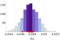
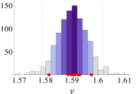
For single-parameter FSS at fixed , the simulation data are uncorrelated and it is sufficient to use a product of independent normal distributions centered on the perfect data set with the same standard deviations as the simulation data to generate the synthetic data sets. In Fig. 12 we show the resulting histograms for the fit of at fixed .
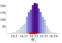
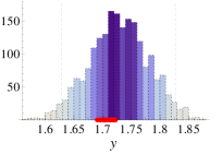
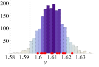
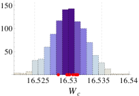
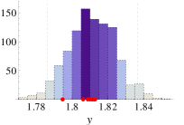
For MFSS the simulation data are correlated and these correlations must be taken into account when generating the synthetic data sets. In this case, the appropriate distribution is a multivariate normal distribution centered on the perfect data set and with the covariance matrix estimated from the simulation data as described in Appendix B. A simple way to generate the necessary correlated data is to use the Cholesky decomposition of the covariance matrix to define an auxiliary set of independent normally distributed random variables with unit variance (see Appendix C). In Fig. 13 we show the histograms for critical parameters obtained from the MFSS of .
Appendix B Calculation of the covariance matrix for correlated data
In this section only we distinguish between the expectation value or population mean indicated by angular brackets, and the sample mean indicated by an overline. To avoid a cumbersome notation we do not make this distinction elsewhere in the paper. In practical calculations, the population mean is always estimated using the sample mean.
The correlation between two random variables and can be characterized in terms of the covariance, defined as
| (46) |
Note that , gives the variance for the variable . From samples , of the pair of random variables, the covariance can be estimated as,Davidson03
| (47) |
Here, the overline indicates the sample mean
| (48) |
and similarly for . We also need the covariance of the sample means. This follows from (46)
| (49) |
Furthermore, we need to consider random variables that are in turn functions of random variables such that
| (50) |
where . Assuming that it is reasonable to linearize the functions in the range of interest, the covariance matrix of the random variables ,
| (51) |
is related to the covariance matrix of the variables by
| (52) |
Here, is the matrix of derivatives
| (53) |
evaluated at .
We now consider the application of the formulae above to the determination of the uncertainties of the GMFE . Correlations only arise between values of this exponent calculated for different coarse-grainings of the same set of samples. Therefore, the covariance matrix for this quantity is block diagonal in disorder and system size . Consider two different coarse-grainings and , and corresponding estimates, and , of the values of this GMFE for these coarse-grainings. Application of the formulae above is then straightforward because is a function of only (see Table 2). The result is
| (54) |
Application of the formulae above to the determination of the uncertainties of the GMFE is more complicated because it is a function of and . The result is
| (55) |
For the formulae are considerably simpler,
| (56) | ||||
| (57) |
Appendix C minimization for correlated data
Let be the result of the -th simulation performed for simulation parameters . The uncertainties and correlations amongst the simulation data are described by a covariance matrix . We fit a model to the simulation data by varying the parameters of the model so as to minimize the chi-squared statistic
| (58) |
In practice it is convenient to perform a Cholesky factorization, , where is an upper triangular matrix, so that can be expressed as the square norm of a vector .
In MFSS, are the values of the GMFE under consideration and . The covariance matrix is calculated as described in Appendix B.
References
- (1) F. Evers and A. D. Mirlin, Rev. Mod. Phys. 80, 1355 (2008).
- (2) S. Faez et al., Phys. Rev. Lett. 103, 155703 (2009).
- (3) M. Morgenstern et al., Phys. Rev. Lett. 89, 136806 (2002).
- (4) K. Hashimoto et al., Phys. Rev. Lett. 101, 256802 (2008).
- (5) E. Cuevas and V. E. Kravtsov, Physical Review B 76, 235119 (2007).
- (6) A. Rodriguez, L. J. Vasquez, K. Slevin, and R. A. Römer, Phys. Rev. Lett. 105, 046403 (2010).
- (7) O. Schenk, M. Bollhöfer, and R. Römer, SIAM Journal of Sci. Comp. 28, 963 (2006).
- (8) M. Bollhöfer and Y. Notay, Comp. Phys. Comm. 177, 951 (2007).
- (9) L. J. Vasquez, A. Rodriguez, and R. A. Römer, Phys. Rev. B 78, 195106 (2008).
- (10) M. Janssen, Int. J. Mod. Phys. B 8, 943 (1994).
- (11) H. Aoki, J. Phys. C 16, L205 (1983).
- (12) M. S. Foster, S. Ryu, and A. W. W. Ludwig, Phys. Rev. B 80, 075101 (2009).
- (13) M. Schreiber and H. Grussbach, Phys. Rev. Lett. 67, 607 (1991).
- (14) H. Grussbach and M. Schreiber, Phys. Rev. B 51, 663 (1995).
- (15) F. Milde, R. A. Römer, and M. Schreiber, Phys. Rev. B 55, 9463 (1997).
- (16) A. Rodriguez, L. J. Vasquez, and R. A. Römer, Phys. Rev. B 78, 195107 (2008).
- (17) A. Rodriguez, L. J. Vasquez, and R. A. Römer, Eur. Phys. J. B 67, 77 (2009).
- (18) J. L. Cardy, Scaling and Renormalization in Statistical Physics (Cambridge University Press, Cambridge, 1996).
- (19) E. Abrahams, P. W. Anderson, D. C. Licciardello, and T. V. Ramakrishnan, Phys. Rev. Lett. 42, 673 (1979).
- (20) P. A. Lee and T. V. Ramakrishnan, Rev. Mod. Phys. 57, 287 (1985).
- (21) K. Yakubo and M. Ono, Phys. Rev. B 58, 9767 (1998).
-
(22)
For 3D exponentially localized states, with a finite localization length , an analytical calculation of the insulating limit for the GMFEs for reveals the following behavior.
For , the moments and saturate and become -independent as . This implies
For we find and asymptotically, which lead to
The latter limit is also obtained for . - (23) A. D. Mirlin, Y. V. Fyodorov, A. Mildenberger, and F. Evers, Phys. Rev. Lett. 97, 046803 (2006).
- (24) Y. V. Fyodorov, A. Ossipov, and A. Rodriguez, J. Stat. Mech. 2009, L12001 (2009).
- (25) F. Evers, A. Mildenberger, and A. D. Mirlin, Phys. Rev. Lett. 101, 116803 (2008).
- (26) A. Mildenberger et al., Phys. Rev. B 75, 094204 (2007).
- (27) A. Mildenberger and F. Evers, Phys. Rev. B 75, 041303 (2007).
- (28) H. Obuse et al., Phys. Rev. Lett. 101, 116802 (2008).
- (29) H. Obuse et al., Phys. Rev. Lett. 98, 156802 (2007).
- (30) A. Rodriguez, L. J. Vasquez, and R. A. Römer, Phys. Rev. Lett. 102, 106406 (2009).
- (31) A. D. Mirlin and Y. V. Fyodorov, Phys. Rev. Lett. 72, 526 (1994).
- (32) A. Richardella et al., Science 327, 665 (2010).
- (33) V. Krachmalnicoff, E. Castanié, Y. De Wilde, and R. Carminati, Phys. Rev. Lett. 105, 183901 (2010).
- (34) D. L. Miller et al., Nature Physics 6, 811 (2010).
- (35) J. Billy et al., Nature 453, 891 (2008).
- (36) G. Roati et al., Nature 453, 895 (2008).
- (37) E. Anderson et al., LAPACK Users’ Guide (Society for Industrial Mathematics, Philadelphia, PA., 1987).
-
(38)
It must be stressed that the scaling laws given here are different from those suggested in the past. In particular for , Eq. (20) for a fixed box size implies a relation of the form
This differs from the scaling law proposed in Refs. Jan94a, ; HucS92,
Moreover, this latter scaling law is in error because the renormalization of the lattice constant (or box size) has been neglected. In fact, for the 3D Anderson model, the latter scaling law produces estimates for which violate the universality of the transition (Ref. VasSRR09, ). - (39) B. Huckestein and L. Schweitzer, Physica A 191, 406 (1992).
- (40) L. J. Vasquez, K. Slevin, A. Rodriguez, and R. A. Römer, Ann. Phys. (Berlin) 18, 901 (2009).
- (41) K. Slevin and T. Ohtsuki, Phys. Rev. Lett. 82, 382 (1999).
- (42) The fits at fixed for , for , and for for do not fully satisfy our stability requirements, as one of the expansions in the stability test gives estimates slightly outside the corresponding confidence intervals. We suspect this is due to the numerical -minimization not being able to resolve two neighboring minima. If we reduce the data set by restricting slightly the range of or the range of , we quickly find stability for the same expansion, giving very similar confidence intervals. Therefore, we include the results for the fits using the whole data set.
- (43) F. Milde, R. A. Römer, M. Schreiber, and V. Uski, Eur. Phys. J. B 15, 685 (2000).
- (44) K. Slevin, T. Ohtsuki, and T. Kawarabayashi, Phys. Rev. Lett. 84, 3915 (2000).
- (45) S. Waffenschmidt, C. Pfleiderer, and H. v. Löhneysen, Phys. Rev. Lett. 83, 3005 (1999).
- (46) S. Anissimova et al., Nature Physics 3, 707 (2007).
- (47) S. V. Kravchenko and M. P. Sarachik, in 50 years of Anderson localization (World Scientific Publishing, 2010), Chap. 17, pp. 361–384.
- (48) F. Wegner, Nucl. Phys. B 316, 663 (1989).
- (49) B. J. Huang and T.-M. Wu, Phys. Rev. E 82, 051133 (2010).
- (50) G. Schubert et al., Phys. Rev. B 81, 155106 (2010).
- (51) S. D. Pinski and R. A. Römer, J. Phys.: Conf. Ser. 286, 012025 (2011).
- (52) A. Eilmes, A. M. Fischer, and R. A. Römer, Phys. Rev. B 77, 245117 (2008).
- (53) J. J. Krich and A. Aspuru-Guzik, Phys. Rev. Lett. 106, 156405 (2011).
- (54) B. J. Huang and T.-M. Wu, Phys. Rev. E 79, 041105 (2009).
- (55) J. Chabé et al., Phys. Rev. Lett. 101, 255702 (2008).
- (56) G. Lemarié et al., Phys. Rev. A 80, 043626 (2009).
- (57) B. Kramer, Phys. Rev. B 47, 9888 (1993).
- (58) H. Hu et al., Nature Physics 4, 945 (2008).
- (59) G. Lemarié et al., Phys. Rev. Lett. 105, 090601 (2010).
- (60) A. C. Davidson, Statistical Models (Cambridge University Press, Cambrigde, UK, 2003).