Exact quantum statistics for electronically nonadiabatic systems using continuous path variables

Abstract

We derive an exact, continuous-variable path integral (PI) representation of the canonical partition function for electronically nonadiabatic systems. Utilizing the Stock-Thoss (ST) mapping for an $N$-level system, matrix elements of the Boltzmann operator are expressed in Cartesian coordinates for both the nuclear and electronic degrees of freedom. The PI discretization presented here properly constrains the electronic Cartesian coordinates to the physical subspace of the mapping. We numerically demonstrate that the resulting PI-ST representation is exact for the calculation of equilibrium properties of systems with coupled electronic and nuclear degrees of freedom. We further show that the PI-ST formulation provides a natural means to initialize semiclassical trajectories for the calculation of real-time thermal correlation functions, which is numerically demonstrated in applications to a series of nonadiabatic model systems.

I Introduction

Electronically nonadiabatic processes lie at the heart of chemical phenomena, including electron solvation dynamics, erb95 ; fw91 ; bs91 ; bs92 ; am09 ; tfm08 energy transfer at metal surfaces,amw04 and radiationless transitions in the condensed phase.hn08 ; fkf76 Elucidating the mechanisms and rates for these processes remains a critical challenge from both the theoretical and experimental perspectives.

In an electronically nonadiabatic process, the Born-Oppenheimer separation of nuclear and electronic motions breaks down, necessitating a description of the coupled motions of the electrons and nuclei. The exponential scaling of exact quantum mechanical methods has motivated the development of numerous mixed quantum-classical (MQC) methods for nonadiabatic dynamics, in which the nuclei are typically treated using classical mechanics and electronic degrees of freedom (DoF) are treated at the quantum mechanical level. These methods, which include the broad classes of mean-fieldpe27 ; cz04 and surface hoppingpp69 ; rk99 ; ad00 ; jct90 ; ovp97 ; awj02 ; mfh95 ; yhw07 approaches, have been succesfully employed in a range of applications. However, it has been shown that processes including non-radiative electronic relaxationer98 and resonance energy transferwhm09 require a consistent description of the coupling between the electronic and nuclear DoF, an inherently challenging task in the MQC framework.jcb00

Semiclassical (SC) methods allow for a dynamically consistent treatment of the electronic and nuclear motion.whm09 ; hdm79 ; gs97 ; gs05 This can be achieved by mapping discrete electronic states to a continuous variable representation using, for instance, spin coherent statesyt75 ; jrk79 ; hk80 ; ms00 or bosonization techniques based on angular momentum theory.th40 ; js65 In particular, Stock and Thoss used the latter approach to derive the mapping Hamiltonian, an exact Cartesian representation of the quantum Hamiltonian for an $N$-level system.gs97 The mapping Hamiltonian has been successfully used in the SC description of processes for which a system initially occupies a pure electronic state.xs97 ; sb051 ; sb052 ; na07 However, use of this approach to calculate real-time quantum thermal correlation functions (TCFs) has relied on initializing SC trajectories to an approximate description of the Boltzmann distribution.hw98 ; jap03 ; eb09 The demonstrated sensitivity aag00 ; gs99 ; gs05 of the calculated TCFs to the initialization scheme indicates that progress is needed to improve the accuracy and generality of this approach.

In this paper, we derive an exact continuous variable PI representation for the Boltzmann distribution of general, N-level systems. This is achieved in the mapping framework using a projection operator to constrain the electronic coordinates to the physical subspace of the mapping. We numerically demonstrate that the resulting PI-ST representation is exact for the calculation of equilibrium properties of two- and three-state systems with coupled electronic and nuclear DoF. We further show that the PI-ST formulation can be used to initialize SC trajectories to an exact quantum Boltzmann distribution, and using the SC initial value representation (SC-IVR) method,whm01 we obtain accurate real-time TCFs for a series of nonadiabatic model systems.

II Theory

II.1 The mapping Hamiltonian

Consider the general $N$-level Hamiltonian operator

$$H=h_{0}(\mathbf{R},\mathbf{P})+\displaystyle\sum_{n,m=1}^{N}V_{nm}(\mathbf{R})|\psi_{n}\rangle\langle\psi_{m}|,$$ (1)

where $(\mathbf{R},\mathbf{P})$ represent the nuclear positions and momenta, $\{\psi_{n}\}$ is the basis of electronic states, and $\{V_{nm}(\mathbf{R})\}$ is the set of potential energy matrix elements. Furthermore, $h_{0}(\mathbf{R},\mathbf{P})=T(\mathbf{P})+V_{0}(\mathbf{R})$, where $T(\mathbf{P})$ is the nuclear kinetic energy operator and $V_{0}(\mathbf{R})$ is a state-independent part of the potential energy.

Following the ST mapping approach,gs97 the $N$-level system is represented by a system of $N$ uncoupled harmonic oscillators (HO), such that

$$|\psi_{n}\rangle\langle\psi_{m}| \rightarrow a_{n}^{+}a_{m}$$ (2)

$$|\psi_{n}\rangle \rightarrow |0_{1}0_{2}\cdots 1_{n}\cdots 0_{N}\rangle.$$ (3)

Here, we have introduced the boson creation and annihilation operators $a_{n}^{+}$ and $a_{n}$, which obey the commutation rules $\left[a_{n}^{+},a_{m}\right]=\delta_{nm}$. We have also introduced the singly excited oscillator (SEO) states $|n\rangle\equiv|0_{1}\cdots 1_{n}\cdots 0_{N}\rangle$, which are $N$-oscillator eigenstates with a single quantum of excitation in the n^th mode. The resulting form of the Hamiltonian operator is

$$H=h_{0}(\mathbf{R},\mathbf{P})+\displaystyle\sum_{n,m=1}^{N}a_{n}^{+}V_{nm}(\mathbf{R})a_{m},$$ (4)

or equivalently in the SEO basis,

$$H=h_{0}(\mathbf{R},\mathbf{P})+\sum_{n,m=1}^{N}|n\rangle V_{nm}(\mathbf{R})\langle m|.$$ (5)

Introducing the Cartesian representation of the boson operators,

$${x}_{n}=\frac{1}{\sqrt{2}}(a_{n}+a_{n}^{+})\;\;\text{and}\;\;{p}_{n}=\frac{i}{\sqrt{2}}(a_{n}^{+}-a_{n}),$$ (6)

we obtain the corresponding Cartesian representation of the Hamiltonian operator,

$$H=h_{0}(\mathbf{R},\mathbf{P})+\frac{1}{2}\displaystyle\sum_{n,m=1}^{N}\left({x}_{n}{x}_{m}+{p}_{n}{p}_{m}-\delta_{nm}\right)V_{nm}(\mathbf{R}).$$ (7)

The mapping Hamiltonian in Eq. (7), also known as the Meyer-Miller-Stock-Thoss Hamiltonian, was originally derived as a classical model for an electronically nonadiabatic system;hdm79 it was later shown to be an exact and general representation for the quantum mechanical Hamiltonian.gs97

II.2 PI discretization

The canonical partition function is obtained from the trace of the Boltzmann operator,

$$Z=\text{Tr}\left[e^{-\beta H}\right],$$ (8)

where $\beta$ is the reciprocal temperature and the trace is taken over the states that span the electronic and nuclear DoF. The resolution of the identity for this space can be expressed as

$$\mathbf{I}=\int d\mathbf{R}\displaystyle\sum_{n=1}^{N}|\mathbf{R},n\rangle\langle\mathbf{R},n|,$$ (9)

where $\mathbf{R}$ indicates nuclear positions and $n$ indicates the SEO state, as before. Repeated insertion of this completeness relation yields a path integral discretization of the partition function,

$$Z =$$

$$\int d\{\mathbf{R}_{\alpha}\}\sum_{\{n_{\alpha}\}=1}^{N}\prod_{\alpha=1}^{P}\langle\mathbf{R}_{\alpha}n_{\alpha}|e^{-\beta_{P}H}|\mathbf{R}_{\alpha+1}n_{\alpha+1}\rangle,\;\;\;$$

where $P$ is the number of time-slices and $\beta_{P}=\beta/P$. We have introduced the notation $\int d\left\{\mathbf{R}_{\alpha}\right\}\equiv\left(\prod_{\alpha=1}^{P}\int d\mathbf{R}_{\alpha}\right)$ and $\sum_{\{n_{\alpha}\}=1}^{N}\equiv\left(\prod_{\alpha=1}^{P}\sum_{n_{\alpha}=1}^{N}\right)$.

The standard Trotter approximationet58 can be used to factorize the matrix elements in this equation, yielding

$$Z = \lim_{P\rightarrow\infty}\int d\left\{\mathbf{R}_{\alpha}\right\}\prod_{\alpha=1}^{P}\left(\frac{MP}{2\pi\beta}\right)^{\frac{f}{2}}e^{-\beta_{P}V_{0}(\mathbf{R}_{\alpha})}$$ (11)

$$\times \text{exp}\left[-\frac{MP}{2\beta}(\mathbf{R}_{\alpha}-\mathbf{R}_{\alpha+1})^{T}\cdot(\mathbf{R}_{\alpha}-\mathbf{R}_{\alpha+1})\right]$$

$$\times \sum_{\{n_{\alpha}\}=1}^{N}\;\prod_{\alpha=1}^{P}\langle n_{\alpha}|e^{-\beta_{P}\mathcal{V}(\mathbf{R}_{\alpha})}|n_{\alpha+1}\rangle,$$

where $f$ is the number of nuclear DoF, $\mathcal{V}(\mathbf{R})=\sum_{n,m=1}^{N}|n\rangle V_{nm}(\mathbf{R})\langle m|$ is the potential energy operator, and we set $\hbar=1$ throughout this paper. In Eq. (11), we have assumed that the Hamiltonian in Eq. (1) is expressed in the diabatic representation, although a similar approach could also be pursued in the adiabatic representation.hdm79 Similar expressions for PI discretization in the basis of discrete electronic states have been obtained. cds99 ; mha01 ; jrs07

The SEO basis in Eq. (11) can be transformed to the Cartesian coordinate basis by first using a projection operator to select the subset of SEO states from the full set of N-oscillator states,

$$\sum_{n=1}^{N}|n\rangle\langle n|=\prod_{i=1}^{N}\left[\sum_{j_{i}=0}^{\infty}|j_{i}\rangle\langle j_{i}|\right]\mathcal{P},$$ (12)

where the projectior operator is defined as

$$\mathcal{P}=\displaystyle\sum_{n=1}^{N}|n\rangle\langle n|.$$ (13)

Then, the full oscillator basis is replaced using

$$\sum_{j_{i}=0}^{\infty}|j_{i}\rangle\langle j_{i}|=\int d\text{x}_{i}|\text{x}_{i}\rangle\langle\text{x}_{i}|,$$ (14)

yielding a transformation from the SEO basis to the Cartesian coordinate basis for the electronic DoF,

$$\sum_{n=1}^{N}|n\rangle\langle n|=\int d\mathbf{x}|\mathbf{x}\rangle\langle\mathbf{x}|\mathcal{P}.$$ (15)

As in Klauder’s work with spin coherent states,jrk97 the projection operator in Eq. (15) constrains electronic coordinates to a specific manifold in phase space. However, PI formulations using spin coherent states have only proven numerically tractable in the semiclassical limit, jrk85 ; jrk97 ; al99 ; ms00 ; aa00 ; vk07 whereas we shall derive a PI formulation that can be used for exact numerical simulations.

Substituting Eq. (15) into Eq. (11), we obtain an exact PI discretization of the canonical partition function in continuous variables,

$$Z = \lim_{P\rightarrow\infty}\int d\left\{\mathbf{R}_{\alpha}\right\}\prod_{\alpha=1}^{P}\left(\frac{MP}{2\pi\beta}\right)^{\frac{f}{2}}e^{-\beta_{P}V_{0}(\mathbf{R}_{\alpha})}$$ (16)

$$\times e^{-\frac{MP}{2\beta}(\mathbf{R}_{\alpha}-\mathbf{R}_{\alpha+1})^{T}.(\mathbf{R}_{\alpha}-\mathbf{R}_{\alpha+1})}\int d\left\{\mathbf{x}_{\alpha}\right\}$$

$$\times \prod_{\alpha=1}^{P}\langle\mathbf{x}_{\alpha}|e^{-\beta_{P}\mathcal{V}(\mathbf{R}_{\alpha})}\mathcal{P}|\mathbf{x}_{\alpha+1}\rangle,$$

leaving only the task of evaluating the matrix elements in the last term to obtain a computationally useful expression.

We note that a short-time approximation to the electronic matrix elements could be performed directly in the Cartesian representation at this stage. However, we find that a more numerically stable result is obtained by making the approximation in the SEO representation, such that

$$\langle\mathbf{x}|e^{-\beta_{P}\mathcal{V}(\mathbf{R})}\mathcal{P}|\mathbf{x}^{\prime}\rangle=\displaystyle\sum_{n,m=1}^{N}\langle\mathbf{x}|n\rangle\mathbf{\mathcal{M}}_{nm}(\mathbf{R})\langle m|\mathbf{x}^{\prime}\rangle,$$ (17)

where $\mathbf{\mathcal{M}}_{nm}(\mathbf{R})=\langle n|e^{-\beta_{P}\mathcal{V}(\mathbf{R})}|m\rangle$. Recognizing that the coordinate space SEO wavefunction is the product of $(N-1)$ ground state HO wavefunctions and one first excited state HO wavefunction, we have

$$\langle\mathbf{x}|n\rangle=\frac{\sqrt{2}}{\pi^{N/4}}\;[\mathbf{x}]_{n}\;e^{-\frac{1}{2}\mathbf{x}^{T}\cdot\mathbf{x}},$$ (18)

where $\left[.\right]_{n}$ denotes the $n^{\text{th}}$ component of the enclosed vector. The Boltzmann matrix element in the SEO representation can then be obtained following textbook procedures,dc87 such that to order $\vartheta(\beta_{P}^{2})$,

$$\mathbf{\mathcal{M}}_{nm}(\mathbf{R})=\left\{\begin{array}[]{cc}e^{-\beta_{P}V_{nn}(\mathbf{R})}&,n=m,\\ -\beta_{P}V_{nm}(\mathbf{R})\;e^{-\beta_{P}V_{nn}(\mathbf{R})}&,n\neq m.\\ \end{array}\right.$$ (19)

In the zero coupling limit, the matrix elements $\mathbf{\mathcal{M}}_{nm}(\mathbf{R})$ assume a diagonal form so that the different components of the electronic position vectors do not mix. The off-diagonal matrix elements are related to the penalty of ring-polymer kink formation, in which neighboring PI time-slices reside on different diabatic electronic surfaces.dc81 ; aoc83

Finally, substituting Eqs. (18) and (19) into Eq. (16), we arrive at the exact, continuous-variable PI-ST representation of the canonical partition function for a nonadiabatic system with $f$ nuclear DoF coupled to $N$ electronic states,

$$Z = \lim_{P\to\infty}\left(\frac{2MP}{\beta\pi^{N+1}}\right)^{\frac{fP}{2}}\int d\left\{\mathbf{R}_{\alpha}\right\}\int d\left\{\mathbf{x}_{\alpha}\right\}$$ (20)

$$\times \prod_{\alpha=1}^{P}\mathcal{A}_{\alpha}\;\mathcal{F}_{\alpha}\;\mathcal{G}_{\alpha},$$

where

$$\mathcal{A}_{\alpha}=e^{-\frac{MP}{2\beta}(\mathbf{R}_{\alpha}-\mathbf{R}_{\alpha+1})^{T}\cdot(\mathbf{R}_{\alpha}-\mathbf{R}_{\alpha+1})}\;e^{-\beta_{P}V_{0}(\mathbf{R}_{\alpha})},$$ (21)

$$\mathcal{F}_{\alpha}=\mathbf{x}_{\alpha}^{T}\;\mathbf{\mathcal{M}}(\mathbf{R}_{\alpha})\;\mathbf{x}_{\alpha+1},\;\;\text{and}$$ (22)

$$\mathcal{G}_{\alpha}=e^{-\mathbf{x}_{\alpha}^{T}\cdot\mathbf{x}_{\alpha}}.$$ (23)

Eqs. (20) - (23) will be used to calculate numerically exact equilibrium properties for nonadiabatic systems.

We note that our PI-ST formulation is different from the result derived in Ref. sb01, , since we include a projection operator to constrain the system to the physical subspace of the mapping. For cases where the system is prepared in a pure SEO state, this constraint is implicitly obeyed, and the two PI representations are equivalent. However, treatment of Boltzmann distributed systems require that the projection operator be explicitly included, as is done in the present study.

III equilibrium simulations

III.1 Implementation details

The equilibrium properties considered in the current paper include the nuclear probability distribution, the state-specific nuclear probability distribution, and the average total energy. All equilibrium simulations were performed using standard path integral Monte Carlo (PIMC) importance sampling techniques, although the use of path integral molecular dynamics (PIMD) methods is also straightforward with the formulation developed here.

The nuclear probability distribution is defined as

$$P(\mathbf{R})=\frac{\text{Tr}[\delta(\mathbf{R}-\hat{\mathbf{R}})e^{-\beta H}]}{\text{Tr}[e^{-\beta H}]}.$$ (24)

Using the PI-ST representation for the Boltzmann operator, we obtain

$$P(\mathbf{R}) =$$ (25)

$$\frac{\int d\{\mathbf{R}_{\alpha}\}\int d\{\mathbf{x}_{\alpha}\}\delta(\mathbf{R}-\mathbf{R}_{P})\displaystyle\prod_{\alpha=1}^{P}\mathcal{A}_{\alpha}\mathcal{G}_{\alpha}\mathcal{F}_{\alpha}}{\int d\left\{\mathbf{R}_{\alpha}\right\}\int\left\{d\mathbf{x}_{\alpha}\right\}\displaystyle\prod_{\alpha=1}^{P}\mathcal{A}_{\alpha}\mathcal{G}_{\alpha}\mathcal{F}_{\alpha}},\;\;\;$$

where $\mathcal{A}_{\alpha}$, $\mathcal{F}_{\alpha}$ and $\mathcal{G}_{\alpha}$ are defined in Eqs. (21) - (23). Importance sampling can then be performed using

$$W(\{\mathbf{x}_{\alpha}\},\{\mathbf{R}_{\alpha}\}) = \displaystyle\prod_{\alpha=1}^{P}\mathcal{A}_{\alpha}\mathcal{G}_{\alpha}|\mathcal{F}_{\alpha}|,$$

where the absolute value in the last term ensures a non-negative sampling function. The expression for the nuclear probability distribution is thus

$$P(\mathbf{R})=\frac{\left<\;\delta(\mathbf{R}-\mathbf{R}_{P})\text{sgn}(\mathcal{F})\;\right>_{W}}{\left<\;\text{sgn}(\mathcal{F})\;\right>_{W}},$$ (26)

where

$$\text{sgn}(\mathcal{F})=\prod_{\alpha=1}^{P}\mathcal{F}_{\alpha}/|\;\mathcal{F}_{\alpha}\;|,$$ (27)

and the angle brackets in Eq. (26) indicate the ensemble average with respect to the distribution $W(\{\mathbf{x}_{\alpha}\},\{\mathbf{R}_{\alpha}\})$.

The state-specific nuclear probability distribution is obtained from the projection of the nuclear probability distribution onto a given electronic state,

$$P(n,\mathbf{R}) = \frac{\text{Tr}[\delta(\mathbf{R}-\hat{\mathbf{R}})|n\rangle\langle n|e^{-\beta H}]}{\text{Tr}[e^{-\beta H}]}$$ (28)

$$= \frac{\langle\;\delta(\mathbf{R}-\mathbf{R}_{P})\tilde{\mathcal{F}_{n}}\;\text{sgn}(\mathcal{F})\;\rangle_{W}}{\langle\;\text{sgn}(\mathcal{F})\;\rangle_{W}},$$

where

$$\tilde{\mathcal{F}_{n}}=\frac{\left[\mathbf{x}_{P}^{T}\mathbf{\mathcal{M}}(\mathbf{R}_{P})\mathbf{x}_{1}\right]_{n}}{\mathbf{x}_{P}^{T}\mathbf{\mathcal{M}}(\mathbf{R}_{P})\mathbf{x}_{1}}.$$ (29)

The elements of the matrix $\mathbf{\mathcal{M}}(\mathbf{R})$ are defined in Eq. (19).

The average total energy of the system is obtained using a primitive energy estimator,

$$\langle E\rangle = -\frac{1}{Z}\frac{\partial Z}{\partial\beta}$$ (30)

$$= \frac{\langle\;(\frac{P}{2\beta}+\tilde{\mathcal{F}}-\frac{\partial\mathcal{A}}{\partial\beta})\;\text{sgn}(\mathcal{F})\;\rangle_{W}}{\langle\;\text{sgn}(\mathcal{F})\;\rangle_{W}},$$

where

$$\tilde{\mathcal{F}} = \displaystyle\sum_{\alpha=1}^{P}\frac{\mathbf{x}_{\alpha}^{T}\;\frac{-\partial\mathbf{\mathcal{M}}(\mathbf{R}_{\alpha})}{\partial\beta}\;\mathbf{x}_{\alpha+1}}{\mathbf{x}_{\alpha}^{T}\mathbf{\mathcal{M}}(\mathbf{R}_{\alpha})\mathbf{x}_{\alpha+1}},$$ (31)

and

$$\frac{\partial\mathcal{A}}{\partial\beta} = \displaystyle\sum_{\alpha=1}^{P}\left[\frac{MP}{2\beta^{2}}(\mathbf{R}_{\alpha}-\mathbf{R}_{\alpha+1})^{T}.(\mathbf{R}_{\alpha}-\mathbf{R}_{\alpha+1})\right.$$ (32)

$$\left.\hskip 108.405pt-\frac{1}{P}V_{0}(\mathbf{R}_{\alpha})\right].$$

III.2 Equilibrium simulation results

The first model that we consider (model I) includes a two-state system coupled to a single vibrational DoF; it is a standard benchmark for the treatment of equilibrium statistics in nonadiabatic systems. jrs07 ; mha01

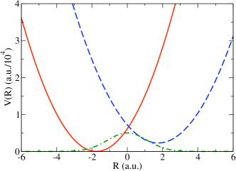
Figure 1: Diabatic potential energy curves for model I, with state 1 in red (solid line), state 2 in blue (dashed line), and the coupling in green (dash-dotted line)

The matrix elements of the diabatic potential operator are

$$V_{ii} = \frac{1}{2}k_{i}(R-R_{i})^{2}+\epsilon_{i}\;\;\;\text{and}$$

$$V_{ij} = ce^{-\alpha(R-R_{ij})^{2}},$$ (33)

where the potential energy parameters are specified in Table 1. The simulation is performed with a nuclear mass of $3600$ a.u. and temperature $T=8$ K. The potential energy curves for Model I are plotted in Fig. 1.

Table 1: Parameters for Model I

Parameter	Value (in a.u.)
$k_{1}$	4 x $10^{-5}$
$k_{2}$	3.2 x $10^{-5}$
$R_{1}$	-1.75
$R_{2}$	1.75
$\epsilon_{1}$	0
$\epsilon_{2}$	2.28 x $10^{-5}$
c	5 x $10^{-5}$
$\alpha$	0.4
$R_{12}$	0

The nuclear probability distribution [Eq. (26)] obtained from a 32 bead PI-ST simulation is shown in Fig. 2(a) and is graphically indistinguishable from a numerically exact discrete variable representation (DVR)dtc92 grid calculation. The tight convergence in this plot was achieved using $5\times 10^{9}$ Monte Carlo (MC) steps, and a similar number of steps was found to be necessary for the corresponding PIMC calculation in the discrete diabatic-state representation. In Fig. 2(b), we show that the state-specific nuclear probability distribution from this simulation also reproduces the exact results. We further calculate the average total energy for Model I and show, in Table 2, that the PI-ST result approaches the exact value in the limit of a large number of beads.

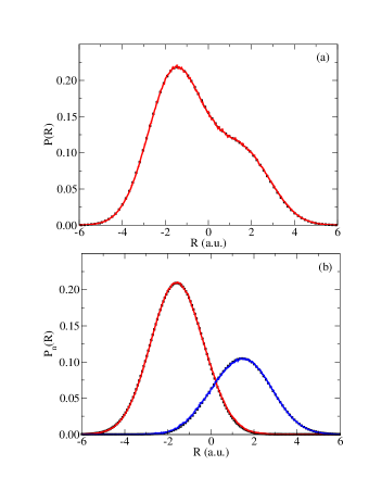
Figure 2: (a) The nuclear probability distribution for model I, obtained using a 32-bead PI-ST simulation (red, solid line) and an exact grid calculation (black squares). (b) The state-specific nuclear probability distribution obtained from the PI-ST simulation, with state 1 in red (solid line, left peak) and state 2 in blue (solid line, right peak); black squares correspond to the exact results.

Table 2: Average Energy for Model I at $T=8$ K

No: of Beads	Energy ($10^{-5}$ a.u.)
8	5.09
16	5.12
32	5.14
Exact	5.145

Model II is a three-state system coupled to a single vibrational DoF. It is based on a model used to simulate ultrafast photoinduced electron-transfer.de04 The model includes a ground (G) electronic state, a locally excited (LE) state that is accessible via photoexcitation, and a charge transfer (CT) state that facilitates radiationless decay to the ground state. The CT state acts as a bridge state between the ground and LE states, and it is coupled to both these states via a constant potential; there is no direct coupling between the ground and LE states.

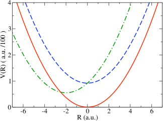
Figure 3: Diabatic potential energy curves for model II, with the G state in red (solid line), the LE state in blue (dashed line) and the CT state in green (dash-dotted line); the constant coupling elements are not shown.

The matrix elements of the diabatic potential operator are

$$V_{i} = \frac{1}{2}\omega_{s}R^{2}+k_{i}R+\epsilon_{i}\;\;\;\text{and}$$

$$V_{ij} = c_{ij},$$ (34)

where $i,j\in\{\text{G},\text{CT},\text{LE}\}$, and the nuclear mass is $544.23$ a.u. The potential energy parameters for Model II are provided in Table 3, and the diabatic three-state potential is shown in Fig. 3. The simulation is performed at $T=1500$ K, chosen such that all three states are thermally accessible.

Table 3: Parameters for Model II

Parameter	Value (in eV)
$\omega_{s}$	0.05
$k_{G}$	0
$k_{CT}$	0.1
$k_{LE}$	0
$\epsilon_{G}$	0
$\epsilon_{CT}$	0.25
$\epsilon_{LE}$	0.25
$c_{G,CT}$	0.02
$c_{CT,LE}$	0.03
$c_{G,LE}$	0

The converged nuclear probability distribution for this model is obtained from a 4-bead calculation and is graphically indistinguishable from the exact results from a DVR grid calculation, as seen in Fig. 4(a). These results were obtained using $10^{9}$ MC steps. The state-specific nuclear probability distributions shown in Fig. 4(b) also reproduce the exact results.

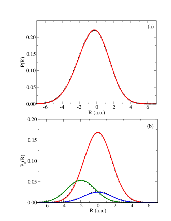
Figure 4: (a) The nuclear probability distribution for model II, obtained using a 4-bead PI-ST simulation (red, solid line) and an exact grid calculation (black squares). (b) The state-specific nuclear probability distribution obtained from the PI-ST simulation with the G state, the CT state and the LE state in red, green and blue (solid lines, in order of decreasing population) respectively.

Further, in Table 4, the results of the average energy calculation are reported, and the exact results are recovered with increasing bead numbers.

Table 4: Average Energy for Model II at T$=1500$ K

No: of Beads	Energy ($10^{-3}$ a.u.)
1	5.54
2	6.63
4	6.69
Exact	6.688

The equilibrium properties calculated for these model systems demonstrate that the PI-ST representation provides a general and exact statistical description of electronically nonadiabatic systems.

IV Thermal Correlation Functions

The PI-ST representation provides a natural means to initialize SC trajectories to an exact quantum Boltzmann distribution for the calculation of real-time TCFs. In this paper, we demonstrate this using the SC-IVR method, which has already been successfully implemented in the mapping framework.xs97 ; xs98 ; na07 However, any trajectory-based model for real-time dynamics could be combined with our exact PI-ST formulation.

A general real-time TCF is expressed as

$$C_{AB}(t)=\frac{1}{Z}\text{Tr}\left[e^{-\beta H}Ae^{iHt}Be^{-iHt}\right],$$ (35)

where $A$ and $B$ are generic operators. Substituting the PI-ST representation for the Boltzmann operator from Eq. (20), the TCF can be written

$$C_{AB}(t)=\frac{1}{Z}\int d\left\{\mathbf{R}_{\alpha}\right\}\int d\left\{\mathbf{x}_{\alpha}\right\}\prod_{\alpha=1}^{P-1}\mathcal{A}_{\alpha}\mathcal{G}_{\alpha}\mathcal{F}_{\alpha}$$

$$\times\;\langle\mathbf{x}_{P},\mathbf{R}_{P}|e^{-\frac{\beta_{P}H}{2}}Ae^{iHt}Be^{-iHt}e^{-\frac{\beta_{P}H}{2}}\mathcal{P}|\mathbf{x}_{1},\mathbf{R}_{1}\rangle,\;\;\;$$ (36)

where $\mathcal{A}_{\alpha}$, $\mathcal{G}_{\alpha}$, and $\mathcal{F}_{\alpha}$ are defined in Eqs. (21-23).

IV.1 Herman-Kluk (HK) IVR

The HK-IVR propagator,mfh84 ; whm01 ; sad06 ; kgk06

$$e^{-iHt}=\left(2\pi\right)^{-(N+f)}\int d\mathbf{z}_{0}\;|\mathbf{z}_{t}\rangle C^{\text{HK}}_{t}(\mathbf{z}_{0})e^{iS_{t}(\mathbf{z}_{0})}\langle\mathbf{z}_{0}|,$$ (37)

is a coherent state approximation to the full coordinate state SC-IVR propagator. Here, $|\mathbf{z}_{0}\rangle=|\mathbf{x}_{0},\mathbf{p}_{0}\rangle|\mathbf{R}_{0},\mathbf{P}_{0}\rangle$ represents the initial electronic and nuclear coherent states of width $\gamma$ and $\Gamma$, respectively, and $|\mathbf{z}_{t}\rangle$ is obtained from classically time-evolving the initial positions and momenta for time $t$. In addition, $S_{t}$ is the classical action, and the HK prefactor is given by

$$C_{t}^{\text{HK}}(\mathbf{z}_{0})=\text{Det}\left[\frac{1}{2}\;\mathbf{g}^{T}\;\frac{\partial\mathbf{z}_{t}}{\partial\mathbf{z}_{0}}\;\mathbf{g^{-1}}\;\right]^{\frac{1}{2}},$$ (38)

where $\mathbf{g}=\left((\gamma,\Gamma)^{1/2}\;,\,i(\gamma,\Gamma)^{-1/2}\right)$.

The forward and backward propagators in Eq. (IV) can be replaced by HK-IVR propagators to obtain an expression with a double phase-space integral over initial conditions,

$$C_{AB}^{\text{HK}}(t)=\frac{\left(2\pi\right)^{-2(N+f)}}{Z}\int d\left\{\mathbf{R}_{\alpha}\right\}\int d\left\{\mathbf{x}_{\alpha}\right\}\prod_{\alpha=1}^{P-1}\mathcal{A}_{\alpha}\mathcal{G}_{\alpha}\mathcal{F}_{\alpha}$$ (39)

$$\times \int d\mathbf{z}_{0}\int d\mathbf{z}_{0}^{\prime}\;e^{i[S_{-t}(\mathbf{z}_{0}^{\prime})+S_{t}(\mathbf{z}_{0})]}C_{-t}(\mathbf{z}_{0}^{\prime})C_{t}(\mathbf{z}_{0})\langle\mathbf{z}_{t}^{\prime}|B|\mathbf{z}_{t}\rangle$$

$$\times \langle\mathbf{x}_{P},\mathbf{R}_{P}|e^{-\beta_{P}H/2}A|\mathbf{z}_{0}^{\prime}\rangle\langle\mathbf{z}_{0}|e^{-\beta_{P}H/2}\mathcal{P}|\mathbf{x}_{1},\mathbf{R}_{1}\rangle.$$

MC integration of the resulting oscillatory integrand is known to be challenging,whm01 and despite several advances in the evaluation of such integrands,nm87 ; xs99 ; re00 ; vj09 the HK-IVR approach is limited to systems with few DoF. Nonetheless, we include the HK-IVR implementation to illustrate the generality of our exact PI initialization approach and to provide a reference semiclassical result to compare against the linearized IVR implementation.

IV.2 Linearized IVR (LSC-IVR)

The LSC-IVR approximation to the coordinate state SC-IVR expression for correlation functions is obtained from a first order expansion of the difference in the actions of the forward and backward trajectories. xs97l ; xs98 The resulting expression corresponds to the classical Wigner model and can be written

$$C_{AB}^{\text{LSC}} (t) =$$

$$\frac{\left(2\pi\right)^{-(N+f)}}{Z}\int d\mathbf{p}_{0}\int d\mathbf{x}_{0}A_{\text{W}}^{\beta}(\mathbf{x}_{0},\mathbf{p}_{0})B_{\text{W}}(\mathbf{x}_{t},\mathbf{p}_{t}),$$

where $A_{\text{W}}^{\beta}=\left(e^{-\beta H}A\right)_{\text{W}}$, and the Wigner transformed operators are obtained by evaluating

$$O_{\text{W}}(\mathbf{x},\mathbf{p})=\int d\Delta\mathbf{x}\langle\mathbf{x}-\frac{\Delta\mathbf{x}}{2}|O|\mathbf{x}+\frac{\Delta\mathbf{x}}{2}\rangle e^{i\mathbf{p}^{T}\cdot\Delta\mathbf{x}}.$$ (41)

The LSC-IVR approximation largely fails to capture quantum coherence effects,xs98 ; whm01 ; na07 but it successfully describes other quantum effects such as zero point energy and tunneling, making it suitable for many condensed phase applications. whm01 ; jl06 ; jl08 ; jl09

The PI-ST representation of the Boltzmann operator can be substituted in the expression for the TCF in Eq. (IV.2) to obtain

$$C_{AB}^{\text{LSC}}(t) = \frac{\left(2\pi\right)^{-(N+f)}}{Z}\int d\left\{\mathbf{R}_{\alpha}\right\}\int d\left\{\mathbf{x}_{\alpha}\right\}\prod_{\alpha=1}^{P-1}\mathcal{A}_{\alpha}\mathcal{G}_{\alpha}\mathcal{F}_{\alpha}$$ (42)

$$\hskip 57.81621pt\times\;\int d\mathbf{z}_{0}\tilde{A}^{\beta}_{\text{W}}(\mathbf{z}_{0})B_{\text{W}}(\mathbf{z}_{t}),$$

where

$$\tilde{A}^{\beta}_{W}(\mathbf{z}_{0})=\int d\Delta\mathbf{x}\int d\Delta\mathbf{R}\;e^{i\mathbf{p}_{0}\cdot\Delta\mathbf{x}+i\mathbf{P}_{0}\cdot\Delta\mathbf{R}}$$ (43)

$$\times \langle\mathbf{x}_{0}-\frac{\Delta\mathbf{x}}{2},\mathbf{R}_{0}-\frac{\Delta\mathbf{R}}{2}|e^{-\frac{\beta_{P}}{2}H}\mathcal{P}|\mathbf{x}_{1},\mathbf{R}_{1}\rangle$$

$$\times \langle\mathbf{x}_{P},\mathbf{R}_{P}|e^{-\frac{\beta_{P}}{2}H}A|\mathbf{x}_{0}+\frac{\Delta\mathbf{x}}{2},\mathbf{R}_{0}+\frac{\Delta\mathbf{R}}{2}\rangle.$$

We recognize that using the exact PI-ST representation of the Boltzmann operator introduces an oscillatory term in the LSC-IVR formulation via $A^{\beta}_{\text{W}}(\mathbf{z}_{0})$. For future applications to large systems, this oscillatory term can be eliminated using techniques such as the Thermal Gaussian Approximation,paf04 for the Boltzmann matrix elements in Eq. (43). Since the remaining $(P-1)$ Boltzmann terms in Eq. (42) will still be treated using the exact PI-ST representation, we expect that this approach would introduce only small deviations from the exact quantum statistical description of a nonadiabatic system.

IV.3 Implementation of PI-ST initialization

Equations (39) and (42) can both be expressed in the form

$$C_{AB}^{\xi}(t)=\frac{1}{Z}\int d\left\{\mathbf{R}_{\alpha}\right\}\int d\left\{\mathbf{x}_{\alpha}\right\}W(\{\mathbf{x}_{\alpha}\},\{\mathbf{R}_{\alpha}\})$$ (44)

$$\hskip 50.58878pt\times\;\;f(\{\mathbf{x}_{\alpha}\},\{\mathbf{R}_{\alpha}\})\Phi^{\xi}(\mathbf{x}_{1},\mathbf{x}_{P},\mathbf{R}_{1},\mathbf{R}_{P},t)$$

$$\vspace{1in}=\left<\;\Phi^{\xi}(\mathbf{x}_{1},\mathbf{x}_{P},\mathbf{R}_{1},\mathbf{R}_{P},t)f(\{\mathbf{x}_{\alpha}\},\{\mathbf{R}_{\alpha}\})\;\right>_{W}$$

$$\hskip 104.79128pt/\left<\;f_{Z}(\{\mathbf{x}_{\alpha}\},\{\mathbf{R}_{\alpha}\})\;\right>_{W},$$

where $W(\{\mathbf{x}_{\alpha}\},\{\mathbf{R}_{\alpha}\})$ is a sampling distribution and $f(\{\mathbf{x}_{\alpha}\},\{\mathbf{R}_{\alpha}\})$ and $f_{Z}(\{\mathbf{x}_{\alpha}\},\{\mathbf{R}_{\alpha}\})$ are weighting factors, all of which emerge from the PI-ST treatment of the Boltzmann operator. The term $\Phi^{\xi}(\mathbf{x}_{1},\mathbf{R}_{1},\mathbf{x}_{P},\mathbf{R}_{P},t)$ in Eq. (44) contains the real-time information obtained from the SC trajectories, and the superscript $\xi\in\{\text{HK,LSC}\}$ indicates which SC approximation is employed.

The calculation of the TCF in Eq. (44) is performed by first generating an ensemble of configurations from the probability distribution $W(\{\mathbf{x}_{\alpha}\},\{\mathbf{R}_{\alpha}\})$. Then, as in standard SC-IVR calculations,whm01 MC importance sampling is used to evaluate $\Phi^{\xi}(\mathbf{x}_{1},\mathbf{R}_{1},\mathbf{x}_{P},\mathbf{R}_{P},t)$. For the HK-IVR implementation,

$$\Phi^{\text{HK}}(\mathbf{x}_{1},\mathbf{x}_{P},\mathbf{R}_{1},\mathbf{R}_{P},t)=$$

$$\;\;N^{\text{HK}}(t)\left<\phi^{\text{HK}}(\mathbf{z}_{0},\mathbf{z}_{t},\mathbf{z}_{0}^{\prime},\mathbf{z}_{t}^{\prime};\mathbf{x}_{1},\mathbf{x}_{P},\mathbf{R}_{1},\mathbf{R}_{P})\right>_{\Pi^{\text{HK}},}$$

and for the LSC-IVR implementation,

$$\Phi^{\text{LSC}}(\mathbf{x}_{1},\mathbf{x}_{P},\mathbf{R}_{1},\mathbf{R}_{P},t)=$$

$$\;\;\;\;\;\;N^{\text{LSC}}(t)\left<\phi^{\text{LSC}}(\mathbf{z}_{0},\mathbf{z}_{t};\mathbf{x}_{1},\mathbf{x}_{P},\mathbf{R}_{1},\mathbf{R}_{P})\right>_{\Pi^{\text{LSC}}},$$

where $\Pi^{\xi}$ is a probability distribution function used to generate an ensemble of initial coordinates and momenta for the SC trajectories, $\phi^{\xi}$ is the corresponding time-dependent estimator, and $N^{\xi}(t)$ is the associated time-dependent normalization term.

In this paper we calculate the electronic state population TCF, $C_{nn}^{\xi}(t)$, where $A=B=|n\rangle\langle n|$ in Eq. (35). For this special case, the detailed form of the functions described above are provided in the appendix.

IV.4 Dynamics simulation results

We calculate the real-time electronic state population TCF using the PI-ST representation of the Boltzmann distribution to initialize SC trajectories for dynamics in the LSC-IVR and HK-IVR frameworks. The first set of results presented are for model III, a simple two-state system described by the Hamiltonian,

$$H=\alpha\sigma_{z}+\Delta\sigma_{x},$$ (47)

where $\sigma_{z}$ and $\sigma_{x}$ are the Pauli matrices. The potential parameters are $\left(\alpha,\Delta\right)~{}=~{}\left(0.5,1\right)$ in a.u. The mapping Hamiltonian for a two-state system assumes a quadratic form for which both the HK-IVR and LSC-IVR formulations are exact. The simulation is performed at a reciprocal temperature of $\beta~{}=~{}1$ a.u., using coherent states of width $\gamma~{}=~{}1$ a.u. SC trajectories are integrated using an Adams-Bashforth-Moulton predictor-corrector integrator.gh76 Exact results are obtained from a DVR grid calculation.

Fig. 5 illustrates that the $C_{11}(t)$ TCF calculated using the LSC-IVR implementation reproduces the exact results, as expected. Simulations performed using the HK-IVR implementation yielded graphically indistinguishable results. These calculations were performed using an 8-bead simulation with $10^{8}$ MC steps for the sampling of the probability distribution $W(\{\mathbf{x},\mathbf{R}\})$. For each of these configurations, ensembles of 120 trajectories and 10 trajectories were generated to obtain the HK-IVR and LSC-IVR TCFs, respectively.

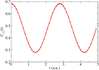
Figure 5: The real-time electronic state population TCF for model III, obtained from the LSC-IVR method with PI-ST initialization (red, solid line) and an exact grid calculation (black squares). Graphically indistinguishable results were also obtained using the HK-IVR method with PI-ST initialization.

Model IV is a two-state system coupled to a single nuclear DoF of mass $M~{}=~{}1$ a.u. The Hamiltonian for this model is

$$H=\frac{P^{2}}{2M}+\frac{1}{2}R^{2}+\alpha R\sigma_{z}+\Delta\sigma_{x},$$ (48)

with parameters (in a.u.) $\alpha~{}=~{}1$, $\Delta~{}=~{}1$, and $\beta~{}=~{}1$. We use coherent states of width $\gamma~{}=~{}1$ a.u and $\Gamma~{}=~{}1$ a.u. for the electronic and nuclear DoF, respectively and 4-bead simulations were performed with $10^{8}$ MC steps for sampling the probability distribution $W(\{\mathbf{x},\mathbf{R}\})$.

In Fig. 6, the TCFs from the HK-IVR and LSC-IVR simulations are compared with the results from an exact DVR grid calculation. The HK-IVR implementation reproduces the exact results with remarkable accuracy, although the calculation required an ensemble of $80,000$ trajectories per equilibrium configuration to converge results up to a time of $2.5$ a.u.; results for longer times would require even larger numbers of trajectories. The LSC-IVR simulation, however, required only $8000$ trajectories per equilibrium configuration to achieve convergence up to $5$ a.u. in time. As expected, the LSC-IVR approximations dampens the oscillations seen in the exact calculation.

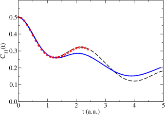
Figure 6: The real-time electronic state population TCF for model IV, obtained from the HK-IVR method with PI-ST initialization (red, dotted line), the LSC-IVR method with PI-ST initialization (blue, solid line), and an exact grid calculation (black, dashed line).

V Conclusions

We have derived an exact PI-ST representation for the Boltzmann statistics of N-level systems using continuous path variables for both the electronic and nuclear DoF. This result is demonstrated to be numerically exact for equilibrium simulations of two- and three-state systems. Additionally, the PI-ST representation is used to initialize trajectories in the SC-IVR framework allowing for the calculation of real-time TCFs with encouraging accuracy. Natural future applications of this methodology include charge transfer reactions in the condensed phase and metal-surface energy transfer processes, for which excited electronic states are thermally accessible.

VI Acknowledgements

The authors sincerely thank Bill Miller for valuable comments and insights. This work was partially supported by a STIR grant from the Army Research Office. T.F.M. additionally acknowledges support from a Camille and Henry Dreyfus Foundation New Faculty Award and an Alfred P. Sloan Foundation Research Fellowship.

Appendix A Electronic state population TCF

The detailed form for all functions used to calculate $C_{nn}^{\xi}(t)$ are provided here. The functions $W(\{\mathbf{x}_{\alpha}\},\{\mathbf{R}_{\alpha}\})$, $f(\{\mathbf{x}_{\alpha}\},\{\mathbf{R}_{\alpha}\})$, and $f_{Z}(\{\mathbf{x}_{\alpha}\},\{\mathbf{R}_{\alpha}\})$ arise from the PI-ST representation of the Boltzmann operator and are identical for both the LSC-IVR and HK-IVR implementations. Specifically,

$$W(\{\mathbf{x}_{\alpha}\},\{\mathbf{R}_{\alpha}\}) = e^{-\beta_{P}V_{0}(\mathbf{R}_{P})/2}\;\mathcal{G}_{P}\;|\mathcal{F}_{P}|$$ (49)

$$\times \prod_{\alpha=1}^{P-1}e^{-\beta_{P}V_{0}(\mathbf{R}_{\alpha})}\;\mathcal{A}_{\alpha}\;\mathcal{G}_{\alpha}\;|\mathcal{F}_{\alpha}|,\;\;\;$$

where $\mathcal{A}_{\alpha}$, $\mathcal{G}_{\alpha}$, and $\mathcal{F}_{\alpha}$ are defined in Eqs. (21-23);

$$f(\{\mathbf{x}_{\alpha}\},\{\mathbf{R}_{\alpha}\})=\frac{e^{-\beta_{P}V_{0}(\mathbf{R}_{1})/2}\text{sgn}(\mathcal{F})}{\mathbf{x}_{P}^{T}\mathbf{\mathcal{M}}(\mathbf{R}_{P})\mathbf{x}_{1}},$$ (50)

where $\text{sgn}(\mathcal{F})$ is defined in Eq.(27) and the elements of $\mathbf{\mathcal{M}}$ defined in Eq. (19); and

$$f_{Z}\left(\{\mathbf{x}_{\alpha}\},\{\mathbf{R}_{\alpha}\}\right)=\text{sgn}(\mathcal{F})e^{-\frac{MP}{2\beta}(\mathbf{R}_{P}-\mathbf{R}_{1})^{T}\cdot(\mathbf{R}_{P}-\mathbf{R}_{1})}\;e^{-\beta_{P}V_{0}(\mathbf{R}_{P})/2}$$ (51)

The terms required to evaluate $\Phi^{\xi}(\mathbf{x}_{1},\mathbf{R}_{1},\mathbf{x}_{P},\mathbf{R}_{P},t)$ in Eqs. (IV.3) and (IV.3) are derived by substituting $A=B=|n\rangle\langle n|$ into Eqs. (39) and (42). In the HK-IVR framework, this yields, the probability distribution function

$$\Pi^{\text{HK}}(\mathbf{z}_{0},\mathbf{z}_{0}^{\prime};\mathbf{R}_{1},\mathbf{R}_{P})=e^{-\frac{\beta}{\beta\Gamma+2MP}(\mathbf{P}_{0}^{T}\cdot\mathbf{P}_{0}+\mathbf{P}^{\prime\;T}_{0}\cdot\mathbf{P}^{\prime}_{0})}$$ (52)

$$e^{-\frac{MP\Gamma}{\beta\Gamma+2MP}\left((\mathbf{R}^{\prime}_{0}-\mathbf{R}_{P})^{T}\cdot(\mathbf{R}^{\prime}_{0}-\mathbf{R}_{P})+(\mathbf{R}_{0}-\mathbf{R}_{1})^{T}\cdot(\mathbf{R}_{0}-\mathbf{R}_{1})\right)}$$

$$e^{-\frac{\gamma}{2(\gamma+1)}(\mathbf{x}_{0}^{T}\cdot\mathbf{x}_{0}+\mathbf{x}^{\prime\;T}_{0}\cdot\mathbf{x}^{\prime}_{0})-\frac{1}{2(\gamma+1)}(\mathbf{p}_{0}^{T}\cdot\mathbf{p}_{0}+\mathbf{p}^{\prime\;T}_{0}\cdot\mathbf{p}^{\prime}_{0})},$$

and the corresponding estimator

$$\phi^{\text{HK}} (\mathbf{z}_{0},\mathbf{z}_{0}^{\prime},\mathbf{z}_{t},\mathbf{z}_{t}^{\prime};\mathbf{x}_{1},\mathbf{x}_{P},\mathbf{R}_{1},\mathbf{R}_{P})=$$ (53)

$$\left[\gamma_{0}\mathbf{x}^{\prime}_{t}-i\mathbf{p}^{\prime}_{t}\right]_{n}\left[\gamma_{0}\mathbf{x}_{t}+i\mathbf{p}_{t}\right]_{n}$$

$$\times \left[\mathbf{x}_{P}^{T}\mathbf{\mathcal{M}}^{\prime}(\mathbf{R}_{P})(\gamma\mathbf{x}^{\prime}_{0}+i\mathbf{p}^{\prime}_{0})\right]_{n}\left((\gamma_{0}\mathbf{x}_{0}-i\mathbf{p}_{0})^{T}\mathbf{\mathcal{M}}^{\prime}(\mathbf{R}_{1})\mathbf{x}_{1}\right)$$

$$\times C_{-t}(\mathbf{z}_{0}^{\prime})C_{t}(\mathbf{z}_{0})e^{i[S_{-t}(\mathbf{z}_{0}^{\prime})+S_{t}(\mathbf{z}_{0})]}$$

$$\times e^{\frac{i}{\gamma+1}\mathbf{p}_{0}^{T}\cdot\mathbf{x}_{0}-\frac{i}{\gamma+1}\mathbf{p}^{\prime\;T}_{0}\cdot\mathbf{x}^{\prime}_{0}-\frac{\Gamma}{4}(\mathbf{R}^{\prime}_{t}-\mathbf{R}_{t})^{T}.(\mathbf{R}^{\prime}_{t}-\mathbf{R}_{t})}$$

$$\times e^{-\frac{1}{4\Gamma}(\mathbf{P}^{\prime}_{t}-\mathbf{P}_{t})^{T}.(\mathbf{P}^{\prime}_{t}-\mathbf{P}_{t})+\frac{i}{2}(\mathbf{P}_{t}+\mathbf{P}^{\prime}_{t})^{T}\cdot(\mathbf{R}^{\prime}_{t}-\mathbf{R}_{t})}$$

$$\times e^{\frac{2iMP}{\beta\Gamma+2MP}\left(\mathbf{P}^{\prime\;T}_{0}\cdot(\mathbf{R}_{P}-\mathbf{R}^{\prime}_{0})-\mathbf{P}_{0}^{T}\cdot(\mathbf{R}_{1}-\mathbf{R}_{0})\right)+\frac{i}{\gamma+1}\left(\mathbf{p}^{\prime\;T}_{t}\cdot\mathbf{x}^{\prime}_{t}-\mathbf{p}_{t}^{T}\cdot\mathbf{x}_{t}\right)}$$

$$\times e^{-\frac{\gamma}{2(\gamma+1)}(\mathbf{x}_{t}^{T}\cdot\mathbf{x}_{t}+\mathbf{x}^{\prime\;T}_{t}\cdot\mathbf{x}^{\prime}_{t})-\frac{1}{2(\gamma+1)}(\mathbf{p}_{t}^{T}\cdot\mathbf{p}_{t}+\mathbf{p}^{\prime\;T}_{t}\cdot\mathbf{p}^{\prime}_{t})},$$

where the elements of the matrix $\mathbf{\mathcal{M}}^{\prime}(\mathbf{R})$ are identical to those of the matrix in Eq. (19) with $\beta~{}\rightarrow~{}\beta/2$.

In the LSC-IVR framework, the probability distribution is

$$\Pi^{\text{LSC}}(\mathbf{z}_{0};\mathbf{R}_{1},\mathbf{R}_{P})=$$ (54)

$$e^{-\frac{2MP}{\beta}\left(\mathbf{R}_{0}-\frac{1}{2}(\mathbf{R}_{P}+\mathbf{R}_{1})\right)^{T}\cdot\left(\mathbf{R}_{0}-\frac{1}{2}(\mathbf{R}_{P}+\mathbf{R}_{1})\right)}$$

$$\times e^{-\frac{\beta}{2MP}\mathbf{P}_{0}^{T}.\mathbf{P}_{0}-\mathbf{x}_{0}^{T}\cdot\mathbf{x}_{0}-\mathbf{p}_{0}^{T}\cdot\mathbf{p}_{0}},$$

and the corresponding estimator is

$$\phi^{\text{LSC}}(\mathbf{z}_{0},\mathbf{z}_{t};\mathbf{x}_{1},\mathbf{x}_{P},\mathbf{R}_{1},\mathbf{R}_{P})=\left(\left[\mathbf{x}_{t}\right]_{n}^{2}+\left[\mathbf{p}_{t}\right]_{n}^{2}-\frac{1}{2}\right)\times$$ (55)

$$\left(\left[\mathbf{x}_{0}+i\mathbf{p}_{0}\right]_{n}(\mathbf{x}_{0}-i\mathbf{p}_{0})^{T}\mathbf{\mathcal{M}}^{\prime}(\mathbf{R}_{1})\mathbf{x}_{1}-\frac{1}{2}\left[\mathbf{\mathcal{M}}^{\prime}(\mathbf{R}_{1})\mathbf{x}_{1}\right]_{n}\right)$$

$$\hskip 28.90755pt\times\left[\mathbf{x}_{P}^{T}\mathbf{\mathcal{M}}^{\prime}(\mathbf{R}_{P})\right]_{n}e^{i\mathbf{P}_{0}^{T}\cdot(\mathbf{R}_{P}-\mathbf{R}_{1})-\mathbf{x}_{t}^{T}\cdot\mathbf{x}_{t}-\mathbf{p}_{t}^{T}\cdot\mathbf{p}_{t}}.$$

A final step in the TCF calculation is to obtain $N^{\xi}(t)$, which is required to both normalize the probability distribution function $\Pi^{\xi}$ and to correct for the non-unitarity of the SC propagator.eac01 Enforcing that the total electronic state population is conserved at all times yields

$$N^{\xi}(t)=\frac{C^{\xi}_{nn}(0)}{\sum_{m=1}^{N}\tilde{C}^{\xi}_{nm}(t)},$$ (56)

where $C_{nn}^{\xi}(0)=\text{Tr}\left[e^{-\beta H}\mathcal{P}_{n}\right]/Z$ can be calculated from an exact PI-ST equilibrium simulation. The terms $\tilde{C}_{nm}^{\xi}(t)$ in Eq. (56) are un-normalized TCFs, such that ${C}_{nm}^{\xi}(t)\equiv N^{\xi}(t)\tilde{C}_{nm}^{\xi}(t)$, where $A=|n\rangle\langle n|$ and $B=|m\rangle\langle m|$ in Eq. (35). These un-normalized terms are obtained following the steps described above, except that the first line on the right-hand side of Eqs. (53) and (55) is modified to include the $m^{\text{th}}$ (rather than the $n^{\text{th}}$) component of vectors $\mathbf{x}_{t},\mathbf{p}_{t},\mathbf{x}_{t}^{\prime},\;\text{and}\;\mathbf{p}_{t}^{\prime}$. The additional computational cost associated with this normalization term is negligible.

References

- (1) E. R. Bittner and P. J. Rossky, J. Chem. Phys. 103, 8130 (1995).
- (2) F. Webster, P. J. Rossky, and R. A. Friesner, Comput. Phys. Commun. 63, 494 (1991).
- (3) B. Space and D. F. Coker, J. Chem. Phys. 94, 1976 (1991).
- (4) B. Space and D. F. Coker, J. Chem. Phys. 96, 652 (1992).
- (5) A. Menzeleev and T. F. Miller III, J. Chem. Phys. 132, 034106 (2010).
- (6) T. F. Miller III, J. Chem. Phys. 129, 194502 (2008).
- (7) A. M. Wodtke, J. C. Tully, and D. J. Auerbach, Int. Rev. Phys. Chem. 23, 513 (2004).
- (8) F. K. Fong, Radiationless processes in Molecules and Condensed Phases, (Springer, Berlin, 1976).
- (9) H. Nakamura, Adv. Chem. Phys. 138, 95 (2008).
- (10) P. Ehrenfest, Z. Phys. 45, 455 (1927).
- (11) C. Zhu, A. W. Jasper, and D. G. Truhlar, J. Chem. Phys. 120, 5543 (2004).
- (12) P. Pechukas, Phys. Rev. 181, 166 (1969).
- (13) R. Kapral and G. Ciccotti, J. Chem. Phys. 110, 8919 (1999).
- (14) A. Donoso and C. C. Martens, J. Chem. Phys. 112, 3980 (2000)
- (15) J. C. Tully, J. Chem. Phys. 93, 1061 (1990).
- (16) O. V. Prezhdo and P. J. Rossky, J. Chem. Phys. 107, 825 (1997).
- (17) A. W. Jasper, S. N. Stechmann, and D. G. Truhlar, J. Chem. Phys. 116, 5424 (2002).
- (18) M. F. Herman, J. Chem. Phys. 103, 8081 (1995).
- (19) Y. H. Wu and M. F. Herman, J. Chem. Phys. 127, 044109 (2007).
- (20) E. Rabani, S. A. Egorov, and B. J. Berne, J. Phys. Chem. A 103, 9539 (1999).
- (21) W. H. Miller, J. Phys. Chem. A 113, 1405 (2009).
- (22) J. C. Burant and J. C. Tully, J. Chem. Phys. 112, 6097 (2000).
- (23) H-D. Meyer and W. H. Miller, J. Chem. Phys. 70, 3214(1979).
- (24) G. Stock and M. Thoss, Phys. Rev. Lett. 78, 578 (1997).
- (25) G. Stock and M. Thoss, Adv. Chem. Phys. 131, 244 (2005).
- (26) Y. Takahashi and F. Shibata, J. Phys. Soc. Japan 38, 656 (1975).
- (27) J. R. Klauder, Phys. Rev. D 19, 2349 (1979).
- (28) H. Kuratsuji and T. Suzuki, J. Math. Phys. 21, 472 (1979).
- (29) M. Stone, K-S. Park, and A. Garg, J. Math. Phys. 41, 8025 (2000).
- (30) T. Holstein and H. Primakoff, Phys. Rev. 58, 1098 (1989).
- (31) J. Schwinger, Quantum Theory of Angular Momentum, edited by L. C. Biedenharn, and H. Van Dam (Academic Press, New York, 1965).
- (32) X. Sun and W. H. Miller, J. Chem. Phys. 106, 6346 (1997).
- (33) S. Bonella, D. Montemayor, and D. F. Coker, Proc. Natl. Acad. Sci U.S.A. 102, 6715 (2005).
- (34) S. Bonella and D. F. Coker, J. Chem. Phys. 122, 194102 (2005).
- (35) N.Ananth, C. Venkataraman, and W. H. Miller, J. Chem. Phys. 127, 084114-1 (2007).
- (36) H. Wang, X. Sun, and W. H. Miller, J. Chem. Phys. 108, 9726 (1998).
- (37) J. A. Poulsen, G. Nyman, and P. J. Rossky, J. Chem. Phys. 119, 12179 (2003).
- (38) E. Bukhman and N. Makri, J. Phys. Chem. A 113, 7183 (2004).
- (39) A. A. Golosov and D. R. Reichman, J. Chem. Phys. 114, 1065 (2001).
- (40) G. Stock and M. Thoss, Phys. Rev. A 59, 64 (1999).
- (41) W. H. Miller, J. Phys. Chem. A 105, 2942 (2001).
- (42) E. Trotter, Proc. Am. Math. Soc. 10, 545 (1958).
- (43) C. D. Schwieters and G. A. Voth, J. Chem. Phys. 111, 2869 (1999).
- (44) M. H. Alexander, J. Chem. Phys. 347, 436 (2001).
- (45) J. R. Schmidt and J. C. Tully, J. Chem. Phys. 127, 094103 (2007).
- (46) J. R. Klauder, Annals of Physics 254, 419 (1997).
- (47) J. R. Klauder and B. S. Skagerstam, Coherent States, Applications in Physics and Mathematical Physics (World Scientific, Singapore, 1985).
- (48) A. Lucke, C. H. Mak, and J. T. Stockburger, J. Chem. Phys. 111, 10843 (1999).
- (49) A. Alscher and H. Grabert, Eur. Phys. J. D 14, 127 (2000).
- (50) V. Krishna, J. Chem. Phys. 126, 134107 (2007).
- (51) D. Chandler, Introduction to Modern Statistical Mechanics (Oxford University Press, New York, 1987).
- (52) D. Chandler and P. G. Wolynes, J. Chem. Phys. 74, 4078 (1981)
- (53) A. O. Caldeira and A. J. Leggett, Ann. Phys. 149, 374456 (1983)
- (54) S. Bonella and D. F. Coker, J. Chem. Phys. 114, 7778 (2001)
- (55) D. T. Colbert and W. H. Miller, J. Chem. Phys. 96, 1982 (1992)
- (56) D. Egorova and W. Domcke, J. Photochem. Photobiol. A 166, 19 (2004)
- (57) M. F. Herman and E. Kluk, Chem. Phys. 91, 27 (1984).
- (58) S. A. Deshpande and G. S. Ezra, J. Phys. A 39, 5067 (2006).
- (59) K. G. Kay, Chem. Phys. 322, 3 (2006).
- (60) N. Makri and W. H. Miller, Chem. Phys. Lett. 139, 10 (1987)
- (61) X. Sun and W. H. Miller, J. Chem. Phys. 110, 6635 (1999).
- (62) R. Egger, L. Mühlbacher, and C. H. Mak, Phys. Rev. E 61, 5961 (2000)
- (63) V. Jadhao and N. Makri, J. Chem. Phys. 132, 104110 (2010)
- (64) X. Sun and W. H. Miller, J. Chem. Phys. 106, 916 (1997).
- (65) X. Sun, H. Wang and W. H. Miller, J. Chem. Phys. 109, 7064 (1998).
- (66) J. Liu and W. H. Miller, J. Chem. Phys. 125, 224104 (2006).
- (67) J. Liu and W. H. Miller, J. Chem. Phys. 128, 144511 (2008).
- (68) J. Liu, W. H. Miller, F. Paesani, W. Zhang, and D. A. Case, J. Chem. Phys. 131, 164509 (2009).
- (69) E. A. Coronado, J. Xing, and W. H. Miller, J. Chem. Phys. 349, 521 (2001)
- (70) G. Hall and J. M. Watt(ed), Modern Numerical Methods for Ordinary Differential Equations (Clarendon Press, Oxford, 1976)
- (71) P. A. Frantsuzov and V. A. Mandelshtam, J. Chem. Phys. 121, 9247 (2004).