Local Scale-Dependent Non-Gaussian Curvature Perturbations at Cubic Order

Abstract

We calculate non-Gaussianities in the bispectrum and trispectrum arising from the cubic term in the local expansion of the scalar curvature perturbation. We compute to three-loop order and for general momenta. A procedure for evaluating the leading behavior of the resulting loop-integrals is developed and discussed. Finally, we survey unique non-linear signals which could arise from the cubic term in the squeezed limit. In particular, it is shown that loop corrections can cause $f_{NL}^{sq.}$ to change sign as the momentum scale is varied. There also exists a momentum limit where $\tau_{NL}<0$ can be realized.

1 Introduction

A variety of new experiments are poised to probe the non-Gaussianity of primordial density fluctuations with unprecedented accuracy. These experiments include the Planck satellite [1] alongside a variety of probes of large scale structure formation [2]. As a result non-Gaussianity can be probed at a wide variety of scales. It thus becomes important to determine which types of models can yield non-Gaussian fluctuations which can be probed at these experiments, and conversely, how measurements from these experiments can be used to constrain inflationary models.

Along this line, considerable work has focused on the local ansatz [3] for non-Gaussian fluctuations, which is realized in many inflationary models. In particular it was shown that non-Gaussianity of the trispectrum is related to non-Gaussianity of the bispectrum through the inequality

$$\tau_{NL}\geq\left({6\over 5}f_{NL}\right)^{2}$$ (1.1)

at tree-level [4], provided the curvature scalar is expanded to quadratic order in Gaussian fields. This became an important constraint, because it implied that measurements at upcoming experiments could potentially rule out the applicability of the local ansatz.

But subsequently it was shown in [5] that this relation is modified to

$$\tau_{NL}\geq{1\over 2}\left({6\over 5}f_{NL}\right)^{2}$$ (1.2)

if one expands to quartic order and includes one-loop corrections. This raises the important question of whether there is indeed a rigid constraint on the trispectrum in the local ansatz, or whether any such constraint can be violated if one computes to sufficiently high loop order. This is especially interesting because it has been shown that in reasonable models loop contributions can dominate over tree-level contributions [6].

In this work, we consider a local ansatz for non-Gaussianity in a multi-field model of inflation (as non-Gaussianity is expected to be very small in single-field models with a standard kinetic term [7]), expanded to cubic order. We calculate the power spectrum, bispectrum and trispectrum up to three-loop order (no higher loop diagram exists for $n$-point functions with $n\leq 4$ at cubic order in the expansion). We will find a variety of interesting features which arise from the non-trivial scale-dependence of loop corrections (see also [8]). In particular, we find that $f_{NL}$ can change sign with momentum scale in the squeezed limit. Moreover, $\tau_{NL}$ can be negative in a particular limit of the external momenta.

In section 2, we review the local ansatz and the various local momentum shapes which are generated at tree-level. In section 3, we describe the formalism for calculating loop diagrams. In section 4, we present results for the computation of the power spectrum, bispectrum and trispectrum to cubic order (detailed calculations are presented in the appendices). We conclude with a discussion of our results in section 5.

2 Local Ansatz For Curvature Perturbations

The local ansatz for the curvature scalar $\zeta$ amounts to the assumption that $\zeta(t,{\bf x})$ can be written as a non-linear function of one or more Gaussian scalar fields $\phi_{i}$, all evaluated at the same space-time point $(t,{\bf x})$. For simplicity, we will assume that there are only two fundamental scalars of interest, the inflaton $\phi$ and an additional field $\chi$.

It was shown in [7] that single-field models of inflation with a standard kinetic term will only yield very small non-Gaussianities. The argument is intuitively quite simple: non-Gaussianities are typically generated by some type of non-linearity in the interaction potential. But the inflaton is constrained to have an extremely flat potential, so the types of non-linearities which could easily generate non-Gaussian curvature fluctuations are constrained by the slow-roll conditions, and non-Gaussianities in single-field models of inflation are thus proportional to the slow-roll parameters.

Of course, there are several ways to avoid this argument, and the one we will focus on is multi-field inflation [9]. In this case, it is assumed that the inflaton’s interactions are largely Gaussian with any non-linearities suppressed by slow-roll parameters. However, there are additional scalar fields which can have significant non-linear interactions, since their interactions are not constrained by the slow-roll conditions. It is these interactions which then feed into scalar curvature perturbations, providing observable non-Gaussianity.

There are many inflationary models which generate non-Gaussianity which is approximately local (see, for example, [9, 10, 11] ). We will not focus on any particular model, however, instead assuming the phenomenological ansatz

$$\zeta(t,{\bf x}) = C_{1}\phi(t,{\bf x})+A_{1}\chi(t,{\bf x})+{1\over 2}A_{2}\left(\chi(t,{\bf x})^{2}-\langle\chi^{2}\rangle\right)+{1\over 6}A_{3}\chi(t,{\bf x})^{3}+\ldots$$ (2.1)

$$\zeta_{\vec{k}} = C_{1}\phi_{\vec{k}}+A_{1}\chi_{\vec{k}}+{1\over 2}\int{d^{3}k^{\prime}\over(2\pi)^{3}}\chi_{\vec{k}^{\prime}}\chi_{\vec{k}-\vec{k}^{\prime}}+{1\over 6}A_{3}\int{d^{3}k^{\prime}\over(2\pi)^{3}}{d^{3}k^{\prime\prime}\over(2\pi)^{3}}\chi_{\vec{k}^{\prime}}\chi_{\vec{k}^{\prime\prime}}\chi_{\vec{k}-\vec{k}^{\prime}-\vec{k}^{\prime\prime}}$$ (2.2)

$$+\ldots$$

In general, of course, the coefficients $C_{1}$, $A_{i}$ can depend weakly on $k$, though this scale-dependence is constrained by bounds on the running of the power spectrum. We will assume that these coefficients are scale-independent. We also assume that the lower bound on momentum is given by $L^{-1}$, where $L$ is the size of the observable universe. Any momenta smaller than $L^{-1}$ correspond to wavelengths larger than the size of the observable universe, which cannot be distinguished from a constant zero mode. A change in the scale of this cutoff $L$ will change the value of the coefficients $A_{i}$, but not the value of the complete $n$-point correlator. Note also that for multi-field models, the scalar curvature fluctuation can exhibit super-Hubble evolution. We will assume, however, that these effects are small.

By assumption both $\phi$ and $\chi$ are Gaussian fields, and their 2-point correlators are given by

$$\langle\phi_{\vec{k}}\phi_{\vec{k}^{\prime}}\rangle=\langle\chi_{\vec{k}}\chi_{\vec{k}^{\prime}}\rangle = (2\pi)^{3}\delta^{3}(\vec{k}+\vec{k}^{\prime}){2\pi^{2}{\cal P}\over k^{3}}$$ (2.3)

$$= (2\pi)^{3}\delta^{3}(\vec{k}+\vec{k}^{\prime})2\pi^{2}{\cal P}F(\vec{k},\vec{k}^{\prime})$$

where

$${\cal P} = \left({H\over 2\pi}\right)^{2}$$

$$F(\vec{k},\vec{k}^{\prime}) = {1\over k^{3}}$$ (2.4)

We see that correlators of the curvature scalar can be written entirely in terms of the above Gaussian correlators. In particular, the lowest order contribution to the 2-point correlator of the curvature scalar is given by

$$\langle\zeta_{\vec{k}}\zeta_{\vec{k}^{\prime}}\rangle = (2\pi)^{3}\delta^{3}(\vec{k}+\vec{k}^{\prime}){2\pi^{2}{\cal P}(C_{1}^{2}+A_{1}^{2})\over k^{3}}$$ (2.5)

It is easiest to visualize this with a diagram (see also [12]), in which each vertex corresponds to an insertion of $\zeta_{\vec{k}}$, while each line corresponds to a 2-point correlator of Gaussian fields. The two-point correlator is then represented by Fig. 1.

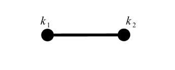
Figure 1: Tree-level representation of the power spectrum.

Similarly, the lowest order diagrams which contribute to the bispectrum are given in Fig. 2. Note that only Gaussian correlators of $\chi$ contribute to these diagrams.

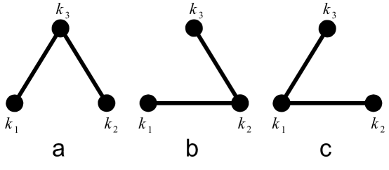
Figure 2: Tree-level contributions to the bispectrum.

The lowest-order contribution to the 3-point correlator is given by

$$\langle\zeta_{\vec{k}_{1}}\zeta_{\vec{k}_{2}}\zeta_{\vec{k}_{3}}\rangle = A_{1}^{2}A_{2}(2\pi^{2}\mathcal{P})^{2}(2\pi)^{3}\delta^{3}(\Sigma_{i}\vec{k}_{i})\left(\frac{1}{k_{1}^{3}k_{2}^{3}}+\text{2 permutations}\right)$$ (2.6)

The momentum shape is thus

$$B(\vec{k}_{1},\vec{k}_{2},\vec{k}_{3}) = {1\over k_{1}^{3}k_{2}^{3}}+{1\over k_{1}^{3}k_{3}^{3}}+{1\over k_{2}^{3}k_{3}^{3}}$$ (2.7)

which is entirely determined by the local shape ansatz.

For the trispectrum there are two tree-level momentum shapes which are possible, because there are two different structures for a diagram connecting 4 vertices with three Gaussian correlators. The first structure, which appears also at quadratic order in the non-linear expansion for $\zeta$, arises from twelve diagrams like Fig. 3a and yields the correlator terms

$$\langle\zeta_{\vec{k}_{1}}\zeta_{\vec{k}_{2}}\zeta_{\vec{k}_{3}}\zeta_{\vec{k}_{4}}\rangle = (2\pi)^{3}\delta^{3}(\Sigma_{i}\vec{k}_{i})A_{2}^{2}A_{1}^{2}(2\pi^{2}\mathcal{P})^{3}\left(\frac{1}{k_{1}^{3}k_{12}^{3}k_{4}^{3}}+\text{11 permutations}\right)$$ (2.8)

where $k_{ij}=|\vec{k}_{i}+\vec{k}_{j}|$. The other shape appears only at cubic order in the expansion, and is given by four diagrams like Fig. 3b. These diagrams yield correlator terms

$$\langle\zeta_{\vec{k}_{1}}\zeta_{\vec{k}_{2}}\zeta_{\vec{k}_{3}}\zeta_{\vec{k}_{4}}\rangle = (2\pi)^{3}\delta^{3}(\Sigma_{i}\vec{k}_{i})A_{3}A_{1}^{3}(2\pi^{2}\mathcal{P})^{3}\left(\frac{1}{k_{1}^{3}k_{3}^{3}k_{4}^{3}}+\text{3 permutations}\right)$$ (2.9)

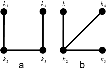
Figure 3: Examples of tree-level contributions to $g_{NL}$ and $\tau_{NL}$.

Note that each tree-level diagram contributes to a term with a different momentum dependence.

We can define the 4-point momentum shapes

$$T(\vec{k}_{1},\vec{k}_{2},\vec{k}_{3},\vec{k}_{4}) = \frac{1}{k_{1}^{3}k_{12}^{3}k_{4}^{3}}+\text{11 permutations}$$

$$G(\vec{k}_{1},\vec{k}_{2},\vec{k}_{3},\vec{k}_{4}) = \frac{1}{k_{1}^{3}k_{3}^{3}k_{4}^{3}}+\text{3 permutations}$$ (2.10)

If we write these tree-level correlators in the form

$$\langle\zeta_{\vec{k}_{1}}\zeta_{\vec{k}_{2}}\rangle = (2\pi)^{3}\delta^{3}(\vec{k}_{1}+\vec{k}_{2})(2\pi^{2}\mathcal{P})F(\vec{k}_{1},\vec{k}_{2})\times N^{2}$$

$$\langle\zeta_{\vec{k}_{1}}\zeta_{\vec{k}_{2}}\zeta_{\vec{k}_{3}}\rangle = (2\pi)^{3}\delta^{3}(\Sigma_{i}\vec{k}_{i})(2\pi^{2}\mathcal{P})^{2}B(\vec{k}_{1},\vec{k}_{2},\vec{k}_{3})\times f$$

$$\langle\zeta_{\vec{k}_{1}}\zeta_{\vec{k}_{2}}\zeta_{\vec{k}_{3}}\zeta_{\vec{k}_{4}}\rangle = (2\pi)^{3}\delta^{3}(\Sigma_{i}\vec{k}_{i})(2\pi^{2}\mathcal{P})^{3}T(\vec{k}_{1},\vec{k}_{2},\vec{k}_{3},\vec{k}_{4})\times t$$ (2.11)

$$+(2\pi)^{3}\delta^{3}(\Sigma_{i}\vec{k}_{i})(2\pi^{2}\mathcal{P})^{3}G(\vec{k}_{1},\vec{k}_{2},\vec{k}_{3},\vec{k}_{4})\times g$$

then we can parameterize non-Gaussianity with the simple definitions

$$f_{NL} \equiv {5\over 6}{f\over N^{4}}$$

$$\tau_{NL} \equiv {t\over N^{6}}$$

$$g_{NL} \equiv {g\over N^{6}}\;.$$ (2.12)

From our tree-level result

$$N^{2} = C_{1}^{2}+A_{1}^{2}>A_{1}^{2}$$

$$f = A_{2}A_{1}^{2}$$

$$t = A_{2}^{2}A_{1}^{2}$$

$$g = A_{3}A_{1}^{3}$$ (2.13)

it is clear that the constraint $\tau_{NL}\geq[(6/5)f_{NL}]^{2}$ holds at tree-level.

3 Calculating Loop Diagrams

However, loop diagrams can correct the correlators in eq. 2, and can do so in a scale-dependent manner. In this section we outline a procedure for evaluating loop contributions to $n$-point curvature perturbation correlators.

There is a single one-loop contribution to the bispectrum at quadratic order in the local expansion, yielding the integral

$$I = \int_{1/L}^{\infty}\frac{d^{3}\vec{k}^{\prime}}{(2\pi)^{3}}{(2\pi^{2}{\cal P})^{3}\over k^{\prime 3}|\vec{k}_{1}-\vec{k}^{\prime}|^{3}|\vec{k}_{2}+\vec{k}^{\prime}|^{3}}\;.$$ (3.1)

This integral can be well approximated [6] by evaluating the integral near the leading logarithmic singularities: ${\vec{k}^{\prime}\sim 0}$, ${\vec{k}^{\prime}\sim\vec{k}_{1}}$ and ${\vec{k}^{\prime}\sim-\vec{k}_{2}}$. Each singularity corresponds to the momentum of one of the three correlators in the loop diagram becoming small. When evaluating a diagram in the leading approximation, we will denote such a correlator with a dashed line (see Fig. 4).

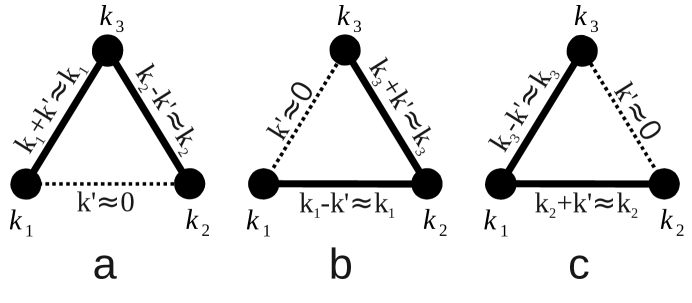
Figure 4: One-loop corrections to the bispectrum up to quadratic order in the expansion.

The resulting expression

$$I \approx (2\pi^{2}{\cal P})^{2}{\cal P}\left[\frac{\ln({\min}(k_{1},k_{2})L)}{k_{1}^{3}k_{2}^{3}}+\frac{\ln({\min}(k_{1},k_{3})L)}{k_{1}^{3}k_{3}^{3}}+\frac{\ln({\min}(k_{2},k_{3})L)}{k_{2}^{3}k_{3}^{3}}\right]$$ (3.2)

captures the leading behavior of this diagram. It is easy to see why the behavior above arises: the integral near each singularity is logarithmic, with one correlator momentum small and the other two correlator momenta being approximately equal to external momenta. The lower limit of integration is set by the IR cutoff $L^{-1}$, while the upper limit is approximately the scale at which at least one other (non-singular) correlator denominator starts to grow with the loop momentum. Above this scale, the denominator will grow as $k_{loop}^{6}$ or greater and the integrand will become small quickly.

More generally, one can derive a prescription for evaluating the leading behavior of an arbitrary $l$-loop contribution to an $n$-point diagram. The leading behavior of the integral is dominated by the limit where the denominators of $l$ of the internal correlators become small. If we denote these correlators by dashed lines, it is clear that in the limit where the momenta associated with the dashed lines vanishes, the remaining solid lines represent the correlators of a tree-level diagram with momenta which are roughly linear combinations of the external insertion momenta. As long as the momenta of the dashed-line correlators are small, the momenta of the solid-line correlators only differ from the tree-level value by a small amount, which has an insignificant effect on those correlators. We may factor out this tree-level contribution, and the leading loop contribution corresponds to a tree-level diagram, multiplied by a loop integral of the form

$$\left({A_{i}A_{j}\over A_{i-1}A_{j-1}}\right)\int_{1/L}^{k_{max_{1}}}{d^{3}k_{loop,1}\over(2\pi)^{3}}{(2\pi^{2}){\cal P}\over k_{loop,1}^{3}}\times\left({A_{k}A_{l}\over A_{k-1}A_{l-1}}\right)\int_{1/L}^{k_{max_{2}}}{d^{3}k_{loop,2}\over(2\pi)^{3}}{(2\pi^{2}){\cal P}\over k_{loop,2}^{3}}$$

$$\times\ldots$$ (3.3)

$$=\left({A_{i}A_{j}\over A_{i-1}A_{j-1}}\right){\cal P}\ln(k_{max,1}L)\times\left({A_{k}A_{l}\over A_{k-1}A_{l-1}}\right){\cal P}\ln(k_{max,2}L)$$

$$\times\ldots$$ (3.4)

where the $k_{loop,i}$ are the momenta of the dashed-line correlators. Each dashed-line correlator is part of exactly one loop which contains only that dashed-line correlator and other solid-line correlators; we denote by $\vec{q}_{j}$ the momenta of the solid-line correlators in that loop, in the limit where all dashed-line correlator momenta vanish (so the solid-line correlators form a tree-diagram, and the $\vec{q}_{j}$ are linear combinations of the external momenta). We then define $k_{max}=\min(q_{j})$ for each dashed-line correlator. As long as $k_{loop,i}<k_{max,i}$ the momenta of the solid-line correlators are largely independent of $k_{loop,i}$ and can be factored out of the integral. For $k_{loop,i}>k_{max,i}$, at least one of the solid-line correlators has a denominator which starts to grow with $k_{loop,i}$. The integrand then scales as $k_{loop,i}^{-6}$ and is small enough that we are justified in ignoring this region of the domain. The factors $A_{i}A_{j}/A_{i-1}A_{j-1}$ account for different vertex coefficients for a loop-diagram, as opposed to a tree-diagram.

One might worry that in a complex multi-loop diagram, the loop integrals would not factorize. But it is straightforward to convince oneself that this is not the case. The leading logarithmic behavior of the integral is dominated by the region where all loop momenta are small, so the integration limits can have only a small dependence on the loop momenta. More physically, one might worry that the correlator denominators might remain small even as the loop momenta became large if two loop momenta cancelled each other in a correlator denominator. But the logarithmic behavior depends on integration over the full loop momentum phase space as one moves away from a singular point; if one restricts the loop momentum phase space by requiring two momenta to cancel each other, then the remaining phase space numerator is insufficient to cancel the $\Pi_{i}k_{loop,i}^{-3}$ behavior of the correlators, and the integrand still becomes small.

We have checked this prescription for the leading logarithmic approximation by comparing it to numerical integrations of the exact integrand for a few specific choices of the external momentum insertions. As in [6] (Appendix B), we transformed momentum integrals to the basis $\vec{n}=\vec{k}L$ and imposed the IR cutoff by setting the integrand to zero when $|\vec{n}-\vec{n}_{pole}|\leq 1$. Choosing $|\vec{k_{small}}L|\approx 10$ and $|\vec{k_{big}}L|\approx 1000$, our approximation of one-loop corrections to squeezed bispectrum and trispectrum differed from numerical values by $\lesssim 1\%$ The leading approximation to the two-loop correction to the bispectrum typically differed from the numerical calculation by $\lesssim 5\%$ ($\lesssim 10\%$ for the trispectrum).

We have shown that this approximation yields the leading behavior of the one-loop 3-point diagram described above. Extending this approximation to $l$-loop $n$-point diagrams, we arrive at the following rules:

1. The numerator for each $n$-point diagram includes

   $$A_{a}A_{b}...A_{z}(2\pi^{2}{\cal P})^{n-1}\mathcal{P}^{l}(2\pi)^{3}\delta^{3}(\Sigma_{i}\vec{k}_{i})$$ (3.5)

   where the coefficients $A_{a}...$ correspond to the coefficients of the $n$ vertices outlined previously.

2. To write the leading log approximation to the diagram, we identify the leading singularities. There are $n+l-1$ Gaussian correlators, of which, in the leading approximation, $n-1$ can be written as solid lines which form a tree-level diagram. The remaining $l$ loop correlators have small momenta and can be written as dashed lines (every choice of which lines are written as dashed corresponds to a different term in the leading approximation). The denominator of each $n$-point diagram includes a cubed product of tree-level momenta.

   $${1\over|\vec{q}_{1}|^{3}...|\vec{q}_{n-1}|^{3}}$$ (3.6)

   where the momenta $q_{i}$ are only functions of the external momenta. This is one term in one of the local momentum shapes for the $n$-point function.

3. Each dashed correlator spans a unique loop containing $m$ tree-level momentum lines $(\vec{q}_{1},...,\vec{q}_{m})$ and no other dashed-line correlators. The momenta $\vec{q}_{i}$ are thus linear combinations of the external momentum insertions, $\vec{k}_{i}$. The integral over each dashed correlator momentum yields a factor

   $$\ln{(\min(\vec{q}_{1},...,\vec{q}_{m})L)}\;.$$ (3.7)

   Note that in the case where a dashed correlator spans only one tree-level line $\vec{k}_{i}$, this simply evaluates to $\ln{(\vec{k}_{i}L)}$.

4. If a set of $r$ dashed lines and $s$ solid lines ($s=0,1$) start at the same vertex and end at the same vertex, this results in a symmetry factor of ${1\over r!}$ if $s=0$, or ${1\over(r-1)!}$ if $s=1$. (Note that while calculating four-point diagrams at the cubic order, $r\leq 2$.)

We see from these rules that each loop comes with a factor of the form

“Loop factor” $$= {A_{i}A_{j}\over A_{i-1}A_{j-1}}{\cal P}\ln(kL)$$ (3.8)

In general, one might expect these factors to be small, since ${\cal P}=(H/2\pi)^{2}$ is necessarily small. However, simple models can be constructed where these loop factors are not small and can even dominate over the tree-level term [6].

4 Results

We can now apply this procedure to the calculation of the power spectrum, bispectrum and trispectrum for local ansatz, to cubic order in the expansion and to 3-loop order.

4.1 Power Spectrum

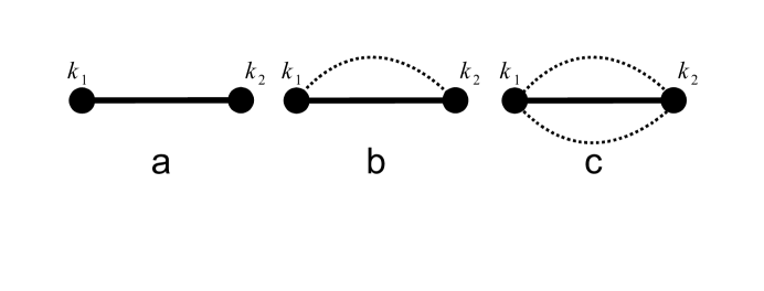
Figure 5: Tree-level, one-loop and two-loop diagrams contributing to the power spectrum.

All diagrams contributing to the power spectrum in the cubic expansion are given in Fig. 5. The full expression for the power spectrum (up to two loop order) is given by

$$\left\langle\zeta_{\vec{k}_{1}}\zeta_{\vec{k}_{2}}\right\rangle = (2\pi)^{3}\delta^{3}(\vec{k_{1}}+\vec{k}_{2})F(\vec{k}_{1},\vec{k}_{2})(2\pi^{2}{\cal P}_{\zeta})$$

$$= (2\pi)^{3}\delta^{3}(\vec{k_{1}}+\vec{k}_{2})F(\vec{k}_{1},\vec{k}_{2})(2\pi^{2}{\cal P})\left[C^{2}+A_{1}^{2}+A_{2}^{2}\mathcal{P}\ln(k_{1}L)+\frac{A_{3}^{2}}{2}\mathcal{P}^{2}\ln(k_{1}L)^{2}\right]$$

Defining $n_{s}=d\ln{\cal P}_{\zeta}/d\ln k$, we find

$$n_{s} = {A_{2}^{2}\mathcal{P}+A_{3}^{2}\mathcal{P}^{2}\ln(kL)\over C^{2}+A_{1}^{2}+A_{2}^{2}\mathcal{P}\ln(kL)+\frac{A_{3}^{2}}{2}\mathcal{P}^{2}\ln(kL)^{2}}$$ (4.2)

COBE measurements of the power spectrum normalization and WMAP bounds on the running of the power spectrum [15] give us the rough constraints

$$N^{2}{\cal P} \sim 10^{-10}$$

$${A_{2}^{2}\mathcal{P}\over N^{2}} \lesssim 10^{-2}$$

$${A_{3}^{2}\mathcal{P}^{2}\ln(kL)\over N^{2}} \lesssim 10^{-2}$$ (4.3)

4.2 Bispectrum

Going beyond tree-level, in general one may write the 3-point correlator as

$$\langle\zeta_{\vec{k}_{1}}\zeta_{\vec{k}_{2}}\zeta_{\vec{k}_{3}}\rangle = (2\pi)^{3}\delta^{3}(\vec{k}_{1}+\vec{k}_{2}+\vec{k}_{3})\langle\zeta_{\vec{k}_{1}}\zeta_{\vec{k}_{2}}\zeta_{\vec{k}_{3}}\rangle^{\prime}$$ (4.4)

and one may then define $f_{NL}$ in the squeezed-limit (see, for example,  [13, 14]) as

$$f_{NL}^{sq.} = {5\over 12}\lim_{\vec{k}_{1}\rightarrow 0}{\langle\zeta_{\vec{k}_{1}}\zeta_{\vec{k}_{2}}\zeta_{\vec{k}_{3}}\rangle^{\prime}\over P_{\zeta}(\vec{k}_{1})P_{\zeta}(\vec{k}_{2})}$$ (4.5)

The full 3-point correlator to third order in $\chi$ is computed in the Appendix, and is given by the expression

$$\langle\zeta_{\vec{k}_{1}}\zeta_{\vec{k}_{2}}\zeta_{\vec{k}_{3}}\rangle = A_{2}(2\pi^{2}\mathcal{P})^{2}(2\pi)^{3}\delta^{3}(\Sigma_{i}\vec{k}_{i}){1\over k_{2}^{3}k_{1}^{3}}\bigg{[}A_{1}^{2}+A_{2}^{2}\mathcal{P}\ln{({\min(k_{1},k_{2})L)}}+A_{1}A_{3}\mathcal{P}\ln{{(k_{1}k_{2}L^{2})}}$$ (4.6)

$$+ A_{3}^{2}\mathcal{P}^{2}\ln{({\min(k_{1},k_{2})L)}}\left(\ln{{(k_{1}k_{2}L^{2})}}+{1\over 2}\ln{({\min(k_{1},k_{2})L)}}\right)\bigg{]}+2\;\rm{perms}$$

It is illuminating to consider this correlator in the squeezed limit $k_{big}\sim k_{2}\sim k_{3}\gg k_{1}\sim k_{sm.}$:

$$\langle\zeta_{\vec{k}_{1}}\zeta_{\vec{k}_{2}}\zeta_{\vec{k}_{3}}\rangle \sim A_{2}A_{1}^{2}(2\pi^{2}\mathcal{P})^{2}(2\pi)^{3}\delta^{3}(\Sigma_{i}\vec{k}_{i}){1\over k_{2}^{3}k_{1}^{3}}\left[1+{A_{2}^{2}\over A_{1}^{2}}\right.\mathcal{P}\ln{({k_{1}L})}+{A_{3}\over A_{1}}\mathcal{P}\ln{{(k_{2}L)}}$$ (4.7)

$$+ \left.{A_{3}^{2}\over A_{1}^{2}}\mathcal{P}^{2}\ln{(k_{1}L)}\ln{(k_{2}L)}\right]+(\vec{k}_{2}\leftrightarrow\vec{k}_{3})$$

In the squeezed limit, the coefficient $f_{NL}$ is then given by

$$f_{NL}^{sq.} = {5\over 6}{A_{2}A_{1}^{2}\over N^{4}}\left[1+{A_{2}^{2}\over A_{1}^{2}}\mathcal{P}\ln{({k_{sm.}L})}+{A_{3}\over A_{1}}\mathcal{P}\ln{{(k_{big}L)}}+{A_{3}^{2}\over A_{1}^{2}}\mathcal{P}^{2}\ln{(k_{sm.}L)}\ln{(k_{big}L)}\right],$$

while in the equilateral limit ($k_{1}\sim k_{2}\sim k_{3}$) we instead get

$$f_{NL}^{equi.} = {5\over 6}{A_{2}A_{1}^{2}\over N^{4}}\left[1+{A_{2}^{2}\over A_{1}^{2}}\mathcal{P}\ln({kL})+2{A_{3}\over A_{1}}\mathcal{P}\ln(kL)+{5\over 2}{A_{3}^{2}\over A_{1}^{2}}\mathcal{P}^{2}(\ln(kL))^{2}\right].$$

The expression for $f_{NL}^{equi.}$ is consistent with the one-loop expression given in [5].

Note that, while in the equilateral limit the loop contribution is always of the same sign as the tree-level contribution, this is not the case for the squeezed limit. If $\ln(k_{sm.}L)\sim 0$, then

$$f_{NL}^{sq.} \rightarrow {5\over 6}{A_{2}A_{1}^{2}\over N^{4}}\left[1+{A_{3}\over A_{1}}\mathcal{P}\ln{{(k_{big}L)}}\right]$$ (4.10)

and the one-loop contribution dominates if $|(A_{3}/A_{1}){\cal P}\ln(k_{big}L)|>1$. If the loop term dominates, then the power spectrum constraints (Eq. 4.1) from COBE and WMAP imply $|f_{NL}^{sq.}|\lesssim 800(\ln k_{big}L)^{1\over 2}$. Note that these constraints would permit a one-loop contribution to the $f_{NL}$ in the squeezed limit which is roughly an order of magnitude larger than that permitted at quadratic order in the equilateral limit [6]. Of course, direct constraints from WMAP on $f_{NL}$ are considerably tighter, requiring $-4<f_{NL}^{sq.}<80$ [16].

It is especially interesting to note that, if $A_{3}/A_{1}$ is negative and $|(A_{3}/A_{1}){\cal P}\ln(k_{big}L)|\sim 1$, then the sign of $f_{NL}^{sq.}$ can change as $k_{big}$ is varied. This could have an especially interesting effect on galaxy bias [17].

4.3 Trispectrum

The full trispectrum to all orders in the cubic expansion (three-loop) is computed in Appendix B (as the full expression is quite large, it will not be reproduced here). We will instead consider the simplest limit, where all the momenta are assumed to be of roughly the same scale ($k_{i}\sim k_{ij}\sim k$). In this limit, we can write

$$\tau_{NL}^{equi.} = {A_{1}^{2}A_{2}^{2}\over N^{6}}\left[1+\left({A_{2}^{2}\over A_{1}^{2}}+4{A_{3}\over A_{1}}+{A_{3}^{2}\over A_{2}^{2}}\right)\right.{\cal P}\ln(kL)+\left({15\over 2}{A_{3}^{2}\over A_{1}^{2}}+2{A_{3}^{3}\over A_{2}^{2}A_{1}}\right)({\cal P}\ln(kL))^{2}$$

$$+\left.{5\over 2}{A_{3}^{4}\over A_{2}^{2}A_{1}^{2}}({\cal P}\ln(kL))^{3}\right]$$

$$g_{NL}^{equi.} = {A_{3}A_{1}^{3}\over N^{6}}\left[1+3{A_{2}^{2}\over A_{1}^{2}}{\cal P}\ln(kL)+\left(3{A_{3}A_{2}^{2}\over A_{1}^{3}}+{3\over 2}{A_{3}^{2}\over A_{1}^{2}}\right)({\cal P}\ln(kL))^{2}+{A_{3}^{3}\over A_{1}^{3}}({\cal P}\ln(kL))^{3}\right]$$

The expression for $\tau_{NL}^{equi.}$ is consistent with the one-loop expression given in [5].

It is again illuminating to consider the behavior of the trispectrum in the limit where the local trispectrum shape $T(\vec{k}_{1},\vec{k}_{2},\vec{k}_{3},\vec{k}_{4})$ becomes large, namely, the elongated quadrilateral limit: $\vec{k}_{1}\sim-\vec{k}_{2}=\vec{k}_{A}$, $\vec{k}_{3}\sim-\vec{k}_{4}=\vec{k}_{B}$, $\vec{k}_{1}+\vec{k}_{2}=\vec{k}_{sum}$, $|\vec{k}_{A}|\geq|\vec{k}_{B}|\gg|\vec{k}_{sum}|$. In this limit

$$G(\vec{k}_{1},\vec{k}_{2},\vec{k}_{3},\vec{k}_{4}) \sim {2\over k_{A}^{3}k_{B}^{6}}$$

$$T(\vec{k}_{1},\vec{k}_{2},\vec{k}_{3},\vec{k}_{4}) \sim {4\over k_{A}^{3}k_{sum}^{3}k_{B}^{3}}$$ (4.12)

We then find

$$\langle\zeta_{\vec{k}_{1}}\zeta_{\vec{k}_{2}}\zeta_{\vec{k}_{3}}\zeta_{\vec{k}_{4}}\rangle \sim (2\pi)^{3}\delta^{3}(\Sigma_{i}\vec{k}_{i})(2\pi^{2}{\cal P})^{3}A_{3}A_{1}^{3}{1\over k_{1}^{3}k_{3}^{3}k_{4}^{3}}\left[1+3{A_{2}^{2}\over A_{1}^{2}}\right.{\cal P}\ln(k_{B}L)$$ (4.13)

$$+3\left({A_{3}A_{2}^{2}\over A_{1}^{3}}+{1\over 2}{A_{3}^{2}\over A_{1}^{2}}\right){\cal P}^{2}(\ln(k_{B}L))^{2}+\left.{A_{3}^{3}\over A_{1}^{3}}{\cal P}^{3}(\ln(k_{B}L))^{3}\right]$$

$$+ (2\pi)^{3}\delta^{3}(\Sigma_{i}\vec{k}_{i})(2\pi^{2}{\cal P})^{3}A_{2}^{2}A_{1}^{2}{1\over k_{1}^{3}k_{12}^{3}k_{4}^{3}}\left[1+\left({A_{2}^{2}\over A_{1}^{2}}+{A_{3}^{2}\over A_{2}^{2}}\right)\right.{\cal P}\ln(k_{sum}L)$$

$$+{A_{3}\over A_{1}}{\cal P}[\ln((k_{A})L)+\ln((k_{B})L)]+{A_{3}^{2}\over A_{1}^{2}}{\cal P}^{2}\ln(k_{A}L)\ln(k_{B}L)$$

$$+{A_{3}^{3}\over A_{2}^{2}A_{1}}{\cal P}^{2}[\ln((k_{A})L)+\ln((k_{B})L)]\ln(k_{sum}L)$$

$$+\left.{A_{3}^{4}\over A_{2}^{2}A_{1}^{2}}{\cal P}^{3}(\ln(k_{B}L))^{2}\ln(k_{sum}L)\right]+\text{permutations}$$

where the first two lines contribute to $g_{NL}$ and the last four lines contribute to $\tau_{NL}$.

If we take the limit $\ln(k_{sum}L)\sim 0$, then we find

$$\tau_{NL}^{sq.}\rightarrow{A_{2}^{2}A_{1}^{2}\over N^{6}}\left[1+{A_{3}\over A_{1}}{\cal P}\ln(k_{A}L)\right]\left[1+{A_{3}\over A_{1}}{\cal P}\ln(k_{B}L)\right]$$ (4.14)

with the dominant loop contributions arising from diagrams “$\tau_{NL}$-e”, “$\tau_{NL}$-g”, and “$\tau_{NL}$-m” in Appendix B.2. If we take $k_{A}=k_{B}\equiv k_{big}$, then the constraint $\tau_{NL}\geq[(6/5)f_{NL}^{sq.}]^{2}$ is necessarily satisfied; at the scale $k_{big}$ where $f_{NL}$ changes sign, $\tau_{NL}$ also vanishes because loop corrections cancel the tree-level contribution.

But if we relax this constraint, allowing $k_{B}<k_{A}$, then $\tau_{NL}$ can be negative. In particular, in the limit $k_{A}=k_{big}$ and ${A_{3}\over A_{1}}{\cal P}\ln(k_{B}L),{A_{3}\over A_{1}}{\cal P}\ln(k_{sum}L)\sim 0$, we find

$$\tau_{NL}^{sq.}\sim{A_{2}^{2}A_{1}^{2}\over N^{6}}\left[1+{A_{3}\over A_{1}}{\cal P}\ln(k_{big}L)\right]$$ (4.15)

where the dominant loop contribution arises from diagram “$\tau_{NL}$-g” in the Appendix B.2. As with the squeezed limit of $f_{NL}$, the one-loop contribution to $\tau_{NL}^{sq.}$ will dominate over the tree-level contribution if $|(A_{3}/A_{1}){\cal P}\ln(k_{big}L)|>1$. The sign of the loop-contribution can be positive or negative, depending on the relative sign of $A_{1}$ and $A_{3}$. As a result, $\tau_{NL}$ could indeed be negative.

This result differs from that stated in [5], because that work assumed that all external momenta are of the same order. We can compare our result to that in [14], where it was claimed that the relation $\tau_{NL}\geq[(6/5)f_{NL}^{sq.}]^{2}$ is always satisfied, due to the fact that a particular covariance matrix is always positive definite. This argument relies on the implicit assumption $k_{A}=k_{B}$ made in [14]. As we have seen above, we reproduce this result if this assumption is made. But this assumption is not required.

Constraints on the power spectrum from COBE and WMAP (Eq. 4.1) constrain the loop contribution to $\tau_{NL}$ to have a magnitude less than $\sim 10^{7}\sqrt{\ln(k_{big}L)}$. As with $f_{NL}$ these constraints in the squeezed limit are much less tight than those at quadratic order in the equilateral limit [6]. Indeed, direct constraints from WMAP already constrain $|\tau_{NL}|\lesssim 10^{4}$  [18].

5 Conclusions

In this work, we have considered the local ansatz for non-Gaussianity in curvature perturbations. We have introduced a simple general formalism for computing higher-order loop corrections to general $n$-point correlators. As expected, the general leading behavior of loop diagrams is the same as for tree-level diagrams, up to logarithmic corrections.

We have illustrated this procedure by computing the curvature power spectrum, bispectrum and trispectrum (expanded to cubic order in fundamental Gaussian fields) to 3-loop order. This calculation has been made for general choices of the external momentum insertions. In particular we conclude that the relation $\tau_{NL}\geq(1/2)[(6/5)f_{NL}]^{2}$ is not necessarily obeyed for all momentum shapes. Furthermore, there exists a squeezed limit (where the $\tau_{NL}$ momentum structure is dominant) where $\tau_{NL}$ can be negative if the loop-contribution dominates. It has also been found that in the squeezed limit the sign of $f_{NL}^{sq.}$ can change as a function of scale. This can have an interesting effect on galaxy bias.

Note that the relationship between $f_{NL}$ and $\tau_{NL}$ depends upon the relative sizes of the external momenta. The constraint $\tau_{NL}\geq[(6/5)f_{NL}^{sq.}]^{2}$ is obtained in the elongated equilateral limit if the external momenta of the trispectrum are taken to all be of the same magnitude, while $\tau_{NL}<0$ can be obtained if there is even a modest hierarchy in the external momenta. The relation $\tau_{NL}\geq(1/2)[(6/5)f_{NL}]^{2}$ is only obeyed at one-loop order if the external momenta are taken to be of the same size. It is important to remember that even if non-Gaussianities are in fact generated by the exact local ansatz (assuming the $A_{i}$ are constant), the bispectrum and trispectrum will not have an exactly local shape; each term in the local shape will be scaled by logarithmic corrections which depend on the particular choice of external momenta. Unless the loop contributions are negligible, the determination of parameters such as $f_{NL}$, $\tau_{NL}$ and $g_{NL}$ from the data will depend on what estimators are used and to which regions of momentum space they are sensitive [19]. It would be interesting to determine what values of these non-Gaussian parameters would actually be yielded by standard estimators as a function of the coefficients $A_{i}$ of the local ansatz.
Acknowledgements
We thank E. Komatsu, L. Leblond, A. Rajaraman and S. Shandera for useful discussions. Preliminary results of this work have been presented at the Aspects Of Inflation Workshop and at the Cosmological non-Gaussianity: Observation Confronts Theory Workshop. We are grateful to the organizers of these workshops, Texas A&M University (MIFP) and the University of Michigan (MCTP) for their hospitality. The work of JB and JK was supported in part by the Department of Energy under Grant DE-FG02-04ER41291.

Appendix A Bispectrum

Computing the bispectrum to two loops in the squeezed limit requires a careful examination of the momentum structure of corresponding IR divergent integrals. In Fig. 6, we exhibit all diagrams contributing to bispectrum terms with leading momentum behavior $1/k_{1}^{3}k_{2}^{3}$. All other bispectrum contributions are related to this result by permutation of the external momenta.

The tree-level contribution to the bispectrum is given by

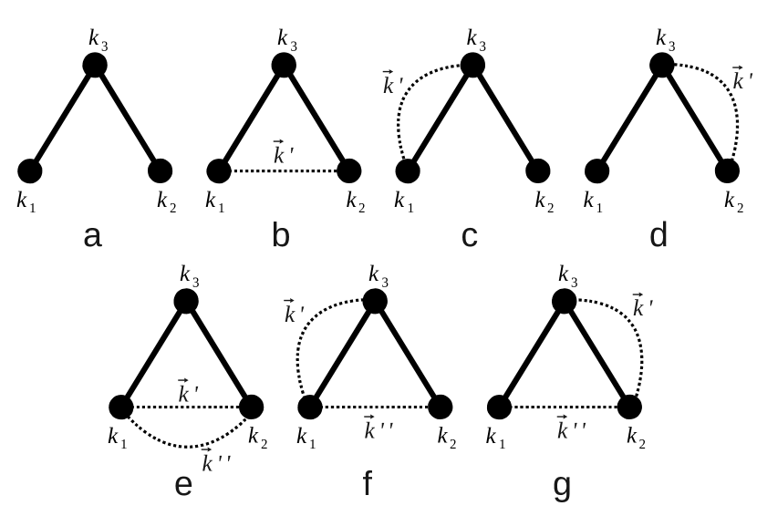
Figure 6: The bispectrum and all distinct corrections up to third order are displayed. Note that particular momentum labels have been chosen for clarity, while for the purpose of calculation all possible momenta permutations are included.

$$\langle\zeta_{\vec{k}_{1}}\zeta_{\vec{k}_{2}}\zeta_{\vec{k}_{3}}\rangle_{f_{NL}a} = \frac{A_{1}^{2}A_{2}(2\pi^{2}\mathcal{P})^{2}}{2}(2\pi)^{6}\int{\frac{d^{3}\vec{k^{\prime}}}{(2\pi)^{3}}\left(\frac{\delta^{3}(\vec{k_{1}}+\vec{k^{\prime}}-\vec{k_{3}})\delta^{3}(\vec{k_{2}}-\vec{k^{\prime}})}{(k_{1}k_{2}k^{\prime}(k_{3}-k^{\prime}))^{3/2}}+1\;\rm{variant}\right)}$$ (A.1)

$$= \frac{2A_{1}^{2}A_{2}(2\pi^{2}\mathcal{P})^{2}}{2}(2\pi)^{3}\delta^{3}(\Sigma_{i}\vec{k_{i}})\frac{1}{k_{1}^{3}k_{2}^{3}}$$

$$= A_{1}^{2}A_{2}(2\pi^{2}\mathcal{P})^{2}(2\pi)^{3}\delta^{3}(\Sigma_{i}\vec{k_{i}})\frac{1}{k_{1}^{3}k_{2}^{3}}$$

The one-loop correction to $f_{NL}$ which uses only terms to second order in $\chi$ is

$$\langle\zeta_{\vec{k}_{1}}\zeta_{\vec{k}_{2}}\zeta_{\vec{k}_{3}}\rangle_{f_{NL}b} = \frac{A_{2}^{3}}{8}\int\frac{d^{3}\vec{k}^{\prime}d^{3}\vec{k}^{\prime\prime}d^{3}\vec{k}^{\prime\prime\prime}}{(2\pi)^{9}}\langle(\chi_{\vec{k}_{1}-\vec{k}^{\prime}}\chi_{\vec{k}^{\prime}})(\chi_{\vec{k}_{2}-\vec{k}^{\prime\prime}}\chi_{\vec{k}^{\prime\prime}})(\chi_{\vec{k}_{3}-\vec{k}^{\prime\prime\prime}}\chi_{\vec{k}^{\prime\prime\prime}})\rangle\;,$$ (A.2)

$$= \frac{A_{2}^{3}(2\pi^{2}\mathcal{P})^{3}}{8}(2\pi)^{3}\delta^{3}(\Sigma_{i}\vec{k_{i}})\int{d^{3}\vec{k}^{\prime}\over(2\pi)^{3}}\left({1\over k^{\prime 3}|\vec{k_{1}}-\vec{k^{\prime}}|^{3}|\vec{k_{2}}+\vec{k^{\prime}}|^{3}}+7\;\rm{perms}\right)$$

$$= A_{2}^{3}(2\pi^{2})^{2}\mathcal{P}^{3}(2\pi)^{3}\delta^{3}(\Sigma_{i}\vec{k_{i}})\frac{\ln({\min}(k_{1},k_{2})L)}{k_{1}^{3}k_{2}^{3}}\;.$$

The 6c piece of the bispectrum includes an integral with two poles instead of three:

$$\langle\zeta_{\vec{k}_{1}}\zeta_{\vec{k}_{2}}\zeta_{\vec{k}_{3}}\rangle_{f_{NL}c} = {1\over 2}A_{3}A_{2}A_{1}(2\pi^{2}\mathcal{P})^{3}(2\pi)^{3}\delta^{3}(\Sigma_{i}\vec{k_{i}})\int{d^{3}\vec{k}^{\prime}\over(2\pi)^{3}}\left({1\over{k^{\prime 3}}|\vec{k_{1}}-\vec{k^{\prime}}|^{3}{k_{2}^{3}}}\right)$$ (A.3)

$$= A_{3}A_{2}A_{1}(2\pi^{2})^{2}\mathcal{P}^{3}(2\pi)^{3}\delta^{3}(\Sigma_{i}\vec{k_{i}})\frac{\ln(\rm k_{1}L)}{k_{1}^{3}k_{2}^{3}}$$

The 6d piece is a mirror of 6c.

$$\langle\zeta_{\vec{k}_{1}}\zeta_{\vec{k}_{2}}\zeta_{\vec{k}_{3}}\rangle_{f_{NL}d} = {1\over 2}A_{3}A_{2}A_{1}(2\pi^{2}\mathcal{P})^{3}(2\pi)^{3}\delta^{3}(\Sigma_{i}\vec{k_{i}})\int{d^{3}\vec{k}^{\prime}\over(2\pi)^{3}}\left({1\over{k^{\prime 3}}|\vec{k_{2}}-\vec{k^{\prime}}|^{3}{k_{1}^{3}}}\right)$$ (A.4)

$$= A_{3}A_{2}A_{1}(2\pi^{2})^{2}\mathcal{P}^{3}(2\pi)^{3}\delta^{3}(\Sigma_{i}\vec{k_{i}})\frac{\ln(\rm k_{2}L)}{k_{1}^{3}k_{2}^{3}}$$

The 6e, 6f, and 6g contributions share the same shape, but must be evaluated separately because the integrals they produce are different. For 6e the expression again relies on which of $|k_{1}|$ and $|k_{2}|$ is smaller.

$$\langle\zeta_{\vec{k}_{1}}\zeta_{\vec{k}_{2}}\zeta_{\vec{k}_{3}}\rangle_{f_{NL}e}$$

$$= {1\over 2}A_{3}^{2}A_{2}(2\pi^{2}\mathcal{P})^{4}(2\pi)^{3}\delta^{3}(\Sigma_{i}\vec{k_{i}})\int\int{d^{3}\vec{k}^{\prime 3}d^{3}\vec{k}^{\prime\prime 3}\over(2\pi)^{6}}\left({1\over{|\vec{k_{1}}-\vec{k^{\prime}}+\vec{k^{\prime\prime}}|^{3}|\vec{k_{2}}+\vec{k^{\prime}}-\vec{k^{\prime\prime}}|^{3}k^{\prime 3}k^{\prime\prime 3}}}\right)$$

$$= {1\over 2}A_{3}^{2}A_{2}(2\pi^{2})^{3}\mathcal{P}^{4}(2\pi)^{3}\delta^{3}(\Sigma_{i}\vec{k_{i}})\int{d^{3}\vec{k}^{\prime 3}\over(2\pi)^{3}}\left({\ln({{\min(k_{1},k_{2})L}})\over{|\vec{k_{1}}-\vec{k^{\prime}}|^{3}|\vec{k_{2}}+\vec{k^{\prime}}|^{3}k^{\prime 3}}}\right)$$

$$= {1\over 2}A_{3}^{2}A_{2}(2\pi^{2})^{2}\mathcal{P}^{4}(2\pi)^{3}\delta^{3}(\Sigma_{i}\vec{k_{i}})\frac{(\ln{({\min(k_{1},k_{2})L}})^{2}}{k_{1}^{3}k_{2}^{3}}$$

The 6f and 6g contributions mirror each other.

$$\langle\zeta_{\vec{k}_{1}}\zeta_{\vec{k}_{2}}\zeta_{\vec{k}_{3}}\rangle_{f_{NL}f} = {1\over 2}A_{3}^{2}A_{2}(2\pi^{2}\mathcal{P})^{4}(2\pi)^{3}\delta^{3}(\Sigma_{i}\vec{k_{i}})\int\int{d^{3}\vec{k}^{\prime 3}d^{3}\vec{k}^{\prime\prime 3}\over(2\pi)^{6}}\left({1\over{|\vec{k_{2}}-\vec{k^{\prime}}|^{3}|\vec{k_{1}}+\vec{k^{\prime}}-\vec{k^{\prime\prime}}|^{3}k^{\prime 3}k^{\prime\prime 3}}}\right)$$ (A.6)

$$= {1\over 2}A_{3}^{2}A_{2}(2\pi^{2})^{3}\mathcal{P}^{4}(2\pi)^{3}\delta^{3}(\Sigma_{i}\vec{k_{i}})\int{d^{3}\vec{k}^{\prime 3}\over(2\pi)^{3}}\left({2\ln({{k_{1}L}})\over{|\vec{k_{2}}-\vec{k^{\prime}}|^{3}|\vec{k_{1}}+\vec{k^{\prime}}|^{3}k^{\prime 3}}}\right)$$

$$= A_{3}^{2}A_{2}(2\pi^{2})^{2}\mathcal{P}^{4}(2\pi)^{3}\delta^{3}(\Sigma_{i}\vec{k_{i}})\frac{\ln({{k_{1}L}})\ln{({\min(k_{1},k_{2})L)}}}{k_{1}^{3}k_{2}^{3}}$$

$$\langle\zeta_{\vec{k}_{1}}\zeta_{\vec{k}_{2}}\zeta_{\vec{k}_{3}}\rangle_{f_{NL}g} = {1\over 2}A_{3}^{2}A_{2}(2\pi^{2}\mathcal{P})^{4}(2\pi)^{3}\delta^{3}(\Sigma_{i}\vec{k_{i}})\int\int{d^{3}\vec{k}^{\prime 3}d^{3}\vec{k}^{\prime\prime 3}\over(2\pi)^{6}}\left({1\over{|\vec{k_{1}}-\vec{k^{\prime}}|^{3}|\vec{k_{2}}+\vec{k^{\prime}}-\vec{k^{\prime\prime}}|^{3}k^{\prime 3}k^{\prime\prime 3}}}\right)$$ (A.7)

$$= {1\over 2}A_{3}^{2}A_{2}(2\pi^{2})^{3}\mathcal{P}^{4}(2\pi)^{3}\delta^{3}(\Sigma_{i}\vec{k_{i}})\int{d^{3}\vec{k}^{\prime 3}\over(2\pi)^{3}}\left({2\ln({{k_{2}L}})\over{|\vec{k_{1}}-\vec{k^{\prime}}|^{3}|\vec{k_{2}}+\vec{k^{\prime}}|^{3}k^{\prime 3}}}\right)$$

$$= A_{3}^{2}A_{2}(2\pi^{2})^{2}\mathcal{P}^{4}(2\pi)^{3}\delta^{3}(\Sigma_{i}\vec{k_{i}})\frac{\ln({{k_{2}L}})\ln{({\min(k_{1},k_{2})L)}}}{k_{2}^{3}k_{1}^{3}}$$

Collecting all terms, the full $f_{NL}$ contribution to third order in $\chi$ is

$$\langle\zeta_{\vec{k}_{1}}\zeta_{\vec{k}_{2}}\zeta_{\vec{k}_{3}}\rangle = A_{2}(2\pi^{2}\mathcal{P})^{2}(2\pi)^{3}\delta^{3}(\Sigma_{i}\vec{k_{i}}){1\over k_{2}^{3}k_{1}^{3}}\bigg{[}A_{1}^{2}+A_{2}^{2}\mathcal{P}\ln{({\min(k_{1},k_{2})L)}}+A_{1}A_{3}\mathcal{P}\ln{{(k_{1}k_{2}L^{2})}}$$ (A.8)

$$+ A_{3}^{2}\mathcal{P}^{2}\ln{({\min(k_{1},k_{2})L)}}\left(\ln{{(k_{1}k_{2}L^{2})}}+\left.{1\over 2}\ln{({\min(k_{1},k_{2})L)}}\right)\right]+2\;\rm{perms}$$

Appendix B Trispectrum

In this appendix we list the complete momentum structure of 4-point correlators up to cubic non-linear order in local expansion of $\zeta$ in Gaussian fields. The complete expansion contains diagrams up to three-loops. Several of these diagrams will contain terms (in the leading log approximation) which contribute to both $g_{NL}$ and $\tau_{NL}$ momentum structures. We will thus compute the contribution to each parameter separately.

B.1 $g_{NL}$

The integrals involved in computing $g_{NL}$ are nearly identical to those used for the bispectrum. The resulting contributions from each diagram are listed below. To save space, henceforth $K\equiv(2\pi)^{3}\delta^{3}(\Sigma_{i}k_{i})$.

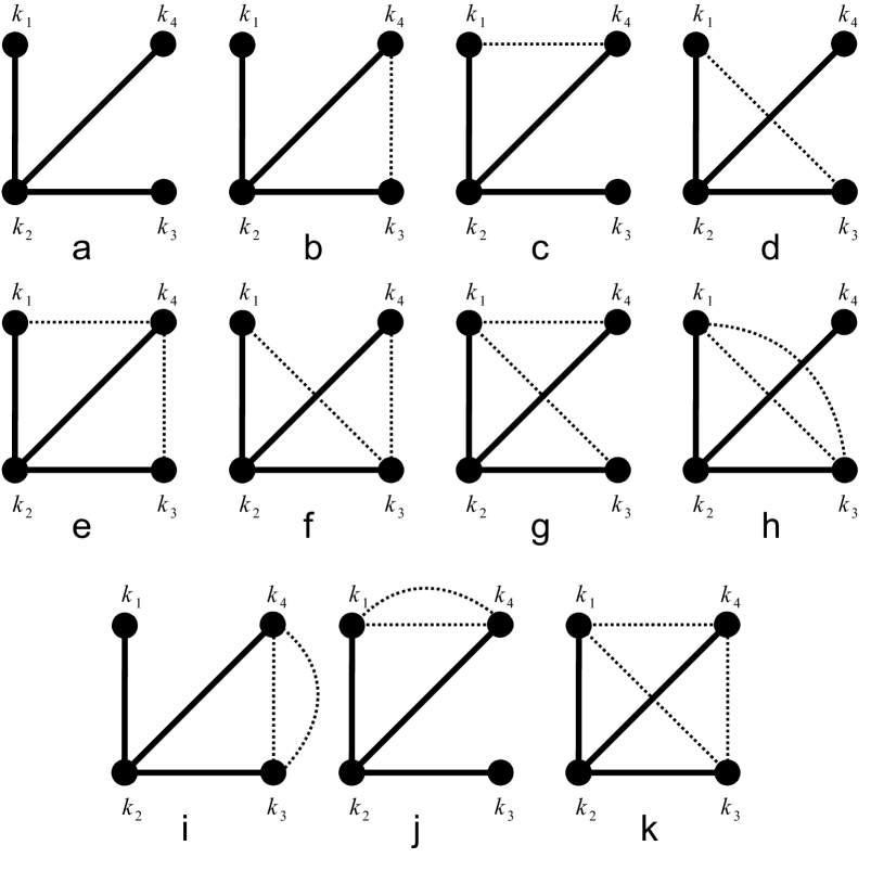
Figure 7: Diagrams contributing to $g_{NL}$ at tree level and all corrections to third order in $\chi$. These diagrams contribute to $1/k_{1}^{3}k_{3}^{3}k_{4}^{3}$ term of the 4-point correlator.

$$\langle\zeta_{\vec{k}_{1}}\zeta_{\vec{k}_{2}}\zeta_{\vec{k}_{3}}\zeta_{\vec{k}_{4}}\rangle_{g_{NL}a} = A_{3}A_{1}^{3}K(2\pi^{2}\mathcal{P})^{3}\frac{1}{k_{1}^{3}k_{4}^{3}k_{3}^{3}}$$ (B.1)

$$\langle\zeta_{\vec{k}_{1}}\zeta_{\vec{k}_{2}}\zeta_{\vec{k}_{3}}\zeta_{\vec{k}_{4}}\rangle_{g_{NL}b} = A_{3}A_{2}^{2}A_{1}K(2\pi^{2})^{3}\mathcal{P}^{4}\frac{\ln{{(\min(k_{3},k_{4})L)}}}{k_{1}^{3}k_{4}^{3}k_{3}^{3}}$$ (B.2)

$$\langle\zeta_{\vec{k}_{1}}\zeta_{\vec{k}_{2}}\zeta_{\vec{k}_{3}}\zeta_{\vec{k}_{4}}\rangle_{g_{NL}c} = A_{3}A_{2}^{2}A_{1}K(2\pi^{2})^{3}\mathcal{P}^{4}\frac{\ln{{(\min(k_{1},k_{4})L)}}}{k_{1}^{3}k_{4}^{3}k_{3}^{3}}$$ (B.3)

$$\langle\zeta_{\vec{k}_{1}}\zeta_{\vec{k}_{2}}\zeta_{\vec{k}_{3}}\zeta_{\vec{k}_{4}}\rangle_{g_{NL}d} = A_{3}A_{2}^{2}A_{1}K(2\pi^{2})^{3}\mathcal{P}^{4}\frac{\ln{{(\min(k_{1},k_{3})L)}}}{k_{1}^{3}k_{4}^{3}k_{3}^{3}}$$ (B.4)

A new mathematical expression in these calculations comes from integrals of the form

$$\int\int{d^{3}k^{\prime}d^{3}k^{\prime\prime}\over(2\pi)^{6}}{1\over{|\vec{k_{4}}-\vec{k^{\prime}}+\vec{k^{\prime\prime}}|^{3}|\vec{k_{1}}+\vec{k^{\prime}}|^{3}|\vec{k_{3}}-\vec{k^{\prime\prime}}|^{3}k^{\prime 3}k^{\prime\prime 3}}}\approx\frac{\ln{{(\min(k_{3},k_{4})L)}}\ln{{(\min(k_{1},k_{4})L)}}}{k_{1}^{3}k_{4}^{3}k_{3}^{3}}$$ (B.5)

$$\langle\zeta_{\vec{k}_{1}}\zeta_{\vec{k}_{2}}\zeta_{\vec{k}_{3}}\zeta_{\vec{k}_{4}}\rangle_{g_{NL}e} = A_{3}^{2}A_{2}^{2}K(2\pi^{2})^{3}\mathcal{P}^{5}\frac{\ln{{(\min(k_{3},k_{4})L)}}\ln{{(\min(k_{1},k_{4})L)}}}{k_{1}^{3}k_{4}^{3}k_{3}^{3}}$$ (B.6)

$$\langle\zeta_{\vec{k}_{1}}\zeta_{\vec{k}_{2}}\zeta_{\vec{k}_{3}}\zeta_{\vec{k}_{4}}\rangle_{g_{NL}f} = A_{3}^{2}A_{2}^{2}K(2\pi^{2})^{3}\mathcal{P}^{5}\frac{\ln{{(\min(k_{3},k_{4})L)}}\ln{{(\min(k_{1},k_{3})L)}}}{k_{1}^{3}k_{4}^{3}k_{3}^{3}}$$ (B.7)

$$\langle\zeta_{\vec{k}_{1}}\zeta_{\vec{k}_{2}}\zeta_{\vec{k}_{3}}\zeta_{\vec{k}_{4}}\rangle_{g_{NL}g} = A_{3}^{2}A_{2}^{2}K(2\pi^{2})^{3}\mathcal{P}^{5}\frac{\ln{{(\min(k_{1},k_{4})L)}}\ln{{(\min(k_{1},k_{3})L)}}}{k_{1}^{3}k_{4}^{3}k_{3}^{3}}$$ (B.8)

$$\langle\zeta_{\vec{k}_{1}}\zeta_{\vec{k}_{2}}\zeta_{\vec{k}_{3}}\zeta_{\vec{k}_{4}}\rangle_{g_{NL}h} = {1\over 2}A_{3}^{3}A_{1}K(2\pi^{2})^{3}\mathcal{P}^{5}\frac{[\ln{{(\min(k_{1},k_{3})L)}}]^{2}}{k_{1}^{3}k_{4}^{3}k_{3}^{3}}$$ (B.9)

$$\langle\zeta_{\vec{k}_{1}}\zeta_{\vec{k}_{2}}\zeta_{\vec{k}_{3}}\zeta_{\vec{k}_{4}}\rangle_{g_{NL}i} = {1\over 2}A_{3}^{3}A_{1}K(2\pi^{2})^{3}\mathcal{P}^{5}\frac{[\ln{{(\min(k_{3},k_{4})L)}}]^{2}}{k_{1}^{3}k_{4}^{3}k_{3}^{3}}$$ (B.10)

$$\langle\zeta_{\vec{k}_{1}}\zeta_{\vec{k}_{2}}\zeta_{\vec{k}_{3}}\zeta_{\vec{k}_{4}}\rangle_{g_{NL}j} = {1\over 2}A_{3}^{3}A_{1}K(2\pi^{2})^{3}\mathcal{P}^{5}\frac{[\ln{{(\min(k_{1},k_{4})L)}}]^{2}}{k_{1}^{3}k_{4}^{3}k_{3}^{3}}$$ (B.11)

Finally, much as in Eq B.5, the fully connected four-point diagram evaluates to

$$\langle\zeta_{\vec{k}_{1}}\zeta_{\vec{k}_{2}}\zeta_{\vec{k}_{3}}\zeta_{\vec{k}_{4}}\rangle_{g_{NL}k}=A_{3}^{4}K(2\pi^{2})^{3}\mathcal{P}^{6}\frac{\ln{{(\min(k_{1},k_{3})L)}}\ln{{(\min(k_{3},k_{4})L)}}\ln{{(\min(k_{1},k_{4})L)}}}{k_{1}^{3}k_{4}^{3}k_{3}^{3}}\;.$$ (B.12)

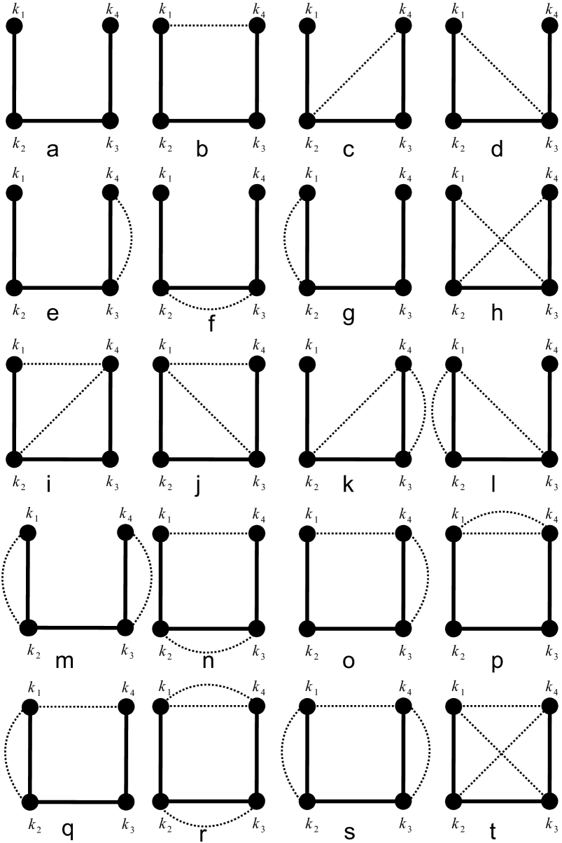
Figure 8: All diagrams contributing to $\tau_{NL}$ at tree level and all corrections up to third order in $\chi$. These diagrams contribute to $1/k_{1}^{3}k_{12}^{3}k_{4}^{3}$ term of the 4-point correlator.

B.2 $\tau_{NL}$

The full calculation for $\tau_{NL}$ involves integrals with poles which owing to the structure of $\tau_{NL}$ are cut off by sums of momentum vectors. Proceeding with the same labelling conventions,

$$\langle\zeta_{\vec{k}_{1}}\zeta_{\vec{k}_{2}}\zeta_{\vec{k}_{3}}\zeta_{\vec{k}_{4}}\rangle_{\tau_{NL}a} = A_{2}^{2}A_{1}^{2}K(2\pi^{2}\mathcal{P})^{3}\frac{1}{k_{1}^{3}k_{12}^{3}k_{4}^{3}}\;,$$ (B.13)

where $k_{12}\equiv|\vec{k}_{1}+\vec{k}_{2}|^{3}$. Using integral approximations already outlined (except often with 4 poles now instead of three),

$$\langle\zeta_{\vec{k}_{1}}\zeta_{\vec{k}_{2}}\zeta_{\vec{k}_{3}}\zeta_{\vec{k}_{4}}\rangle_{\tau_{NL}b} = A_{2}^{4}K(2\pi^{2})^{3}\mathcal{P}^{4}\frac{\ln{({\min(k_{1},k_{12},k_{4})L})}}{k_{1}^{3}k_{12}^{3}k_{4}^{3}}$$ (B.14)

$$\langle\zeta_{\vec{k}_{1}}\zeta_{\vec{k}_{2}}\zeta_{\vec{k}_{3}}\zeta_{\vec{k}_{4}}\rangle_{\tau_{NL}c} = A_{3}A_{2}^{2}A_{1}K(2\pi^{2})^{3}\mathcal{P}^{4}\frac{\ln{({\min(k_{12},k_{4})L})}}{k_{1}^{3}k_{12}^{3}k_{4}^{3}}$$ (B.15)

$$\langle\zeta_{\vec{k}_{1}}\zeta_{\vec{k}_{2}}\zeta_{\vec{k}_{3}}\zeta_{\vec{k}_{4}}\rangle_{\tau_{NL}d} = A_{3}A_{2}^{2}A_{1}K(2\pi^{2})^{3}\mathcal{P}^{4}\frac{\ln{({\min(k_{12},k_{1})L})}}{k_{1}^{3}k_{12}^{3}k_{4}^{3}}$$ (B.16)

$$\langle\zeta_{\vec{k}_{1}}\zeta_{\vec{k}_{2}}\zeta_{\vec{k}_{3}}\zeta_{\vec{k}_{4}}\rangle_{\tau_{NL}e} = A_{3}A_{2}^{2}A_{1}K(2\pi^{2})^{3}\mathcal{P}^{4}\frac{\ln{({k_{4}}L)}}{k_{1}^{3}k_{12}^{3}k_{4}^{3}}$$ (B.17)

$$\langle\zeta_{\vec{k}_{1}}\zeta_{\vec{k}_{2}}\zeta_{\vec{k}_{3}}\zeta_{\vec{k}_{4}}\rangle_{\tau_{NL}f} = A_{3}^{2}A_{1}^{2}K(2\pi^{2})^{3}\mathcal{P}^{4}\frac{\ln{({k_{12}}L)}}{k_{1}^{3}k_{12}^{3}k_{4}^{3}}$$ (B.18)

$$\langle\zeta_{\vec{k}_{1}}\zeta_{\vec{k}_{2}}\zeta_{\vec{k}_{3}}\zeta_{\vec{k}_{4}}\rangle_{\tau_{NL}g} = A_{3}A_{2}^{2}A_{1}K(2\pi^{2})^{3}\mathcal{P}^{4}\frac{\ln{({k_{1}}L)}}{k_{1}^{3}k_{12}^{3}k_{4}^{3}}$$ (B.19)

$$\langle\zeta_{\vec{k}_{1}}\zeta_{\vec{k}_{2}}\zeta_{\vec{k}_{3}}\zeta_{\vec{k}_{4}}\rangle_{\tau_{NL}h} = A_{3}^{2}A_{2}^{2}K(2\pi^{2})^{3}\mathcal{P}^{5}\frac{\ln{({\min(k_{12},k_{4})L})}\ln{({\min(k_{12},k_{1})L})}}{k_{1}^{3}k_{12}^{3}k_{4}^{3}}$$ (B.20)

$$\langle\zeta_{\vec{k}_{1}}\zeta_{\vec{k}_{2}}\zeta_{\vec{k}_{3}}\zeta_{\vec{k}_{4}}\rangle_{\tau_{NL}i} = A_{3}^{2}A_{2}^{2}K(2\pi^{2})^{3}\mathcal{P}^{5}\frac{\ln{({\min(k_{12},k_{4})L})}\ln{({\min(k_{1},k_{12},k_{4})L})}}{k_{1}^{3}k_{12}^{3}k_{4}^{3}}$$

$$\langle\zeta_{\vec{k}_{1}}\zeta_{\vec{k}_{2}}\zeta_{\vec{k}_{3}}\zeta_{\vec{k}_{4}}\rangle_{\tau_{NL}j} = A_{3}^{2}A_{2}^{2}K(2\pi^{2})^{3}\mathcal{P}^{5}\frac{\ln{({\min(k_{12},k_{1})L})}\ln{({\min(k_{1},k_{12},k_{4})L})}}{k_{1}^{3}k_{12}^{3}k_{4}^{3}}$$

$$\langle\zeta_{\vec{k}_{1}}\zeta_{\vec{k}_{2}}\zeta_{\vec{k}_{3}}\zeta_{\vec{k}_{4}}\rangle_{\tau_{NL}k} = A_{3}^{3}A_{1}K(2\pi^{2})^{3}\mathcal{P}^{5}\frac{\ln{({k_{4}L})}\ln{({\min(k_{12},k_{4})L})}}{k_{1}^{3}k_{12}^{3}k_{4}^{3}}$$ (B.23)

$$\langle\zeta_{\vec{k}_{1}}\zeta_{\vec{k}_{2}}\zeta_{\vec{k}_{3}}\zeta_{\vec{k}_{4}}\rangle_{\tau_{NL}l} = A_{3}^{3}A_{1}K(2\pi^{2})^{3}\mathcal{P}^{5}\frac{\ln{({k_{1}L})}\ln{({\min(k_{12},k_{1})L})}}{k_{1}^{3}k_{12}^{3}k_{4}^{3}}$$ (B.24)

$$\langle\zeta_{\vec{k}_{1}}\zeta_{\vec{k}_{2}}\zeta_{\vec{k}_{3}}\zeta_{\vec{k}_{4}}\rangle_{\tau_{NL}m} = A_{3}^{2}A_{2}^{2}K(2\pi^{2})^{3}\mathcal{P}^{5}\frac{\ln{({k_{1}}L)}\ln{({k_{4}}L)}}{k_{1}^{3}k_{12}^{3}k_{4}^{3}}$$ (B.25)

$$\langle\zeta_{\vec{k}_{1}}\zeta_{\vec{k}_{2}}\zeta_{\vec{k}_{3}}\zeta_{\vec{k}_{4}}\rangle_{\tau_{NL}n} = A_{3}^{2}A_{2}^{2}K(2\pi^{2})^{3}\mathcal{P}^{5}\frac{\ln{({k_{12}L})}\ln{({\min(k_{1},k_{12},k_{4})L})}}{k_{1}^{3}k_{12}^{3}k_{4}^{3}}$$ (B.26)

$$\langle\zeta_{\vec{k}_{1}}\zeta_{\vec{k}_{2}}\zeta_{\vec{k}_{3}}\zeta_{\vec{k}_{4}}\rangle_{\tau_{NL}o} = A_{3}^{2}A_{2}^{2}K(2\pi^{2})^{3}\mathcal{P}^{5}\frac{\ln{({k_{4}L})}\ln{({\min(k_{1},k_{12},k_{4})L})}}{k_{1}^{3}k_{12}^{3}k_{4}^{3}}$$ (B.27)

$$\langle\zeta_{\vec{k}_{1}}\zeta_{\vec{k}_{2}}\zeta_{\vec{k}_{3}}\zeta_{\vec{k}_{4}}\rangle_{\tau_{NL}p} = {1\over 2}A_{3}^{2}A_{2}^{2}K(2\pi^{2})^{3}\mathcal{P}^{5}\frac{\ln{({\min(k_{1},k_{12},k_{4})L})}^{2}}{k_{1}^{3}k_{12}^{3}k_{4}^{3}}$$ (B.28)

$$\langle\zeta_{\vec{k}_{1}}\zeta_{\vec{k}_{2}}\zeta_{\vec{k}_{3}}\zeta_{\vec{k}_{4}}\rangle_{\tau_{NL}q} = A_{3}^{2}A_{2}^{2}K(2\pi^{2})^{3}\mathcal{P}^{5}\frac{\ln{({k_{1}L})}\ln{({\min(k_{1},k_{12},k_{4})L})}}{k_{1}^{3}k_{12}^{3}k_{4}^{3}}$$ (B.29)

$$\langle\zeta_{\vec{k}_{1}}\zeta_{\vec{k}_{2}}\zeta_{\vec{k}_{3}}\zeta_{\vec{k}_{4}}\rangle_{\tau_{NL}r} = {1\over 2}A_{3}^{4}K(2\pi^{2})^{3}\mathcal{P}^{6}\frac{\ln{({k_{12}L})}\ln{({\min(k_{1},k_{12},k_{4})L})^{2}}}{k_{1}^{3}k_{12}^{3}k_{4}^{3}}$$ (B.30)

$$\langle\zeta_{\vec{k}_{1}}\zeta_{\vec{k}_{2}}\zeta_{\vec{k}_{3}}\zeta_{\vec{k}_{4}}\rangle_{\tau_{NL}s} = A_{3}^{4}K(2\pi^{2})^{3}\mathcal{P}^{6}\frac{\ln{({k_{4}L})}\ln{({k_{4}L})}\ln{({\min(k_{1},k_{12},k_{4})L})}}{k_{1}^{3}k_{12}^{3}k_{4}^{3}}$$ (B.31)

$$\langle\zeta_{\vec{k}_{1}}\zeta_{\vec{k}_{2}}\zeta_{\vec{k}_{3}}\zeta_{\vec{k}_{4}}\rangle_{\tau_{NL}t} = A_{3}^{4}K(2\pi^{2})^{3}\mathcal{P}^{6}\frac{\ln{({\min(k_{1},k_{12},k_{4})L})}\ln{({\min(k_{1},k_{12})L})}\ln{({\min(k_{12},k_{4})L})}}{k_{1}^{3}k_{12}^{3}k_{4}^{3}}$$

References

- [1] Planck Surveyor - http://planck.esa.int .
- [2] J. E. Carlstrom et al., arXiv:0907.4445 [astro-ph.IM]; Baryon oscillation spectroscopic survey (boss), http://cosmology.lbl.gov/BOSS/ ; T. Abbott et al. [Dark Energy Survey Collaboration], arXiv:astro-ph/0510346; Hobby eberly telescope dark energy experiment (hetdex), http://www.as.utexas.edu/hetdex/ ; Physics of the accelerating universe (pau), http://www.ice.csic.es/research/PAU/PAU-welcome.html ; LSST http://www.lsst.org .
- [3] D. S. Salopek, J. R. Bond, Phys. Rev. D42, 3936-3962 (1990); L. Verde, L. M. Wang, A. Heavens and M. Kamionkowski, Mon. Not. Roy. Astron. Soc. 313, L141 (2000) [arXiv:astro-ph/9906301]; E. Komatsu and D. N. Spergel, Phys. Rev. D 63, 063002 (2001) [arXiv:astro-ph/0005036].
- [4] T. Suyama, M. Yamaguchi, PHRVA,D77,023505. 2008 D77, 023505 (2008). [arXiv:0709.2545 [astro-ph]].
- [5] N. S. Sugiyama, E. Komatsu and T. Futamase, arXiv:1101.3636 [gr-qc].
- [6] J. Kumar, L. Leblond and A. Rajaraman, JCAP 1004, 024 (2010) [arXiv:0909.2040 [astro-ph.CO]].
- [7] A. Gangui, F. Lucchin, S. Matarrese and S. Mollerach, Astrophys. J. 430, 447 (1994) [arXiv:astro-ph/9312033]; V. Acquaviva, N. Bartolo, S. Matarrese, A. Riotto, Nucl. Phys. B667, 119-148 (2003) [astro-ph/0209156]; J. M. Maldacena, JHEP 0305, 013 (2003) [arXiv:astro-ph/0210603].
- [8] L. Boubekeur and D. H. Lyth, Phys. Rev. D 73, 021301 (2006) [arXiv:astro-ph/0504046]; C. T. Byrnes, K. Y. Choi and L. M. H. Hall, JCAP 0902, 017 (2009) [arXiv:0812.0807 [astro-ph]]; C. T. Byrnes, S. Nurmi, G. Tasinato and D. Wands, JCAP 1002, 034 (2010) [arXiv:0911.2780 [astro-ph.CO]]; A. Rajaraman, J. Kumar and L. Leblond, Phys. Rev. D 82, 023525 (2010) [arXiv:1002.4214 [hep-th]]; C. T. Byrnes, M. Gerstenlauer, S. Nurmi, G. Tasinato and D. Wands, JCAP 1010, 004 (2010) [arXiv:1007.4277 [astro-ph.CO]].
- [9] G. I. Rigopoulos, E. P. S. Shellard and B. J. W. van Tent, Phys. Rev. D 76, 083512 (2007) [arXiv:astro-ph/0511041]; D. Seery and J. E. Lidsey, JCAP 0509, 011 (2005) [arXiv:astro-ph/0506056]; F. Vernizzi and D. Wands, JCAP 0605, 019 (2006) [arXiv:astro-ph/0603799]; T. Battefeld and R. Easther, JCAP 0703, 020 (2007) [arXiv:astro-ph/0610296]; K. Y. Choi, L. M. H. Hall and C. van de Bruck, JCAP 0702, 029 (2007) [arXiv:astro-ph/0701247]; S. Yokoyama, T. Suyama and T. Tanaka, JCAP 0707, 013 (2007) [arXiv:0705.3178 [astro-ph]]; S. Yokoyama, T. Suyama and T. Tanaka, Phys. Rev. D 77, 083511 (2008) [arXiv:0711.2920 [astro-ph]]; M. Sasaki, Prog. Theor. Phys. 120, 159 (2008) [arXiv:0805.0974 [astro-ph]]; B. Dutta, L. Leblond and J. Kumar, Phys. Rev. D 78, 083522 (2008) [arXiv:0805.1229 [hep-th]]; H. R. S. Cogollo, Y. Rodriguez and C. A. Valenzuela-Toledo, JCAP 0808, 029 (2008) [arXiv:0806.1546 [astro-ph]]; Y. Rodriguez and C. A. Valenzuela-Toledo, Phys. Rev. D 81, 023531 (2010) [arXiv:0811.4092 [astro-ph]]; C. T. Byrnes, K. Y. Choi and L. M. H. Hall, JCAP 0810, 008 (2008) [arXiv:0807.1101 [astro-ph]]; C. T. Byrnes and K. Y. Choi, Adv. Astron. 2010, 724525 (2010) [arXiv:1002.3110 [astro-ph.CO]]; Q. G. Huang, JCAP 1012, 017 (2010) [arXiv:1009.3326 [astro-ph.CO]].
- [10] D. H. Lyth, C. Ungarelli and D. Wands, Phys. Rev. D 67, 023503 (2003) [arXiv:astro-ph/0208055]; K. Ichikawa, T. Suyama, T. Takahashi and M. Yamaguchi, Phys. Rev. D 78, 023513 (2008) [arXiv:0802.4138 [astro-ph]]; M. Beltran, Phys. Rev. D 78, 023530 (2008) [arXiv:0804.1097 [astro-ph]]; Q. G. Huang, JCAP 0811, 005 (2008) [arXiv:0808.1793 [hep-th]]; K. Enqvist, S. Nurmi, O. Taanila and T. Takahashi, JCAP 1004, 009 (2010) [arXiv:0912.4657 [astro-ph.CO]]; K. Enqvist and T. Takahashi, JCAP 0912, 001 (2009) [arXiv:0909.5362 [astro-ph.CO]]; L. Alabidi, K. Malik, C. T. Byrnes and K. Y. Choi, JCAP 1011, 037 (2010) [arXiv:1002.1700 [astro-ph.CO]]; A. Chambers, S. Nurmi and A. Rajantie, JCAP 1001, 012 (2010) [arXiv:0909.4535 [astro-ph.CO]].
- [11] G. Dvali, A. Gruzinov and M. Zaldarriaga, Phys. Rev. D 69, 023505 (2004) [arXiv:astro-ph/0303591]; M. Zaldarriaga, Phys. Rev. D 69, 043508 (2004) [arXiv:astro-ph/0306006].
- [12] C. T. Byrnes, K. Koyama, M. Sasaki, D. Wands, JCAP 0711, 027 (2007) [arXiv:0705.4096 [hep-th]]; S. Yokoyama, T. Suyama, T. Tanaka, JCAP 0902, 012 (2009) [arXiv:0810.3053 [astro-ph]].
- [13] K. M. Smith and M. Zaldarriaga, arXiv:astro-ph/0612571.
- [14] K. M. Smith, M. LoVerde and M. Zaldarriaga, arXiv:1108.1805 [astro-ph.CO].
- [15] E. Komatsu et al. [WMAP Collaboration], Astrophys. J. Suppl. 180, 330 (2009) [arXiv:0803.0547 [astro-ph]].
- [16] K. M. Smith, L. Senatore and M. Zaldarriaga, JCAP 0909, 006 (2009) [arXiv:0901.2572 [astro-ph]].
- [17] see, for example, N. Kaiser, Astrophys. J. 284, L9-L12 (1984); N. Dalal, O. Dore, D. Huterer and A. Shirokov, Phys. Rev. D 77, 123514 (2008) [arXiv:0710.4560 [astro-ph]]; A. Slosar, C. Hirata, U. Seljak, S. Ho and N. Padmanabhan, JCAP 0808, 031 (2008) [arXiv:0805.3580 [astro-ph]]; S. Shandera, N. Dalal, D. Huterer, JCAP 1103, 017 (2011). [arXiv:1010.3722 [astro-ph.CO]].
- [18] J. Smidt, A. Amblard, C. T. Byrnes, A. Cooray, A. Heavens, and D. Munshi, Phys. Rev. D 81, 123007 (2010) [arXiv:1004.1409 [astro-ph.CO]].
- [19] M. Kamionkowski, T. L. Smith, A. Heavens, Phys. Rev. D83, 023007 (2011). [arXiv:1010.0251 [astro-ph.CO]].