Detection of ultrafast oscillations in Superconducting Point-Contacts by means of Supercurrent Measurements

Abstract

We present a microscopic calculation of the nondissipative current through a superconducting quantum point contact coupled to a mechanical oscillator. Using the nonequilibrium Keldysh Green function approach, we determine the current-phase relation. The latter shows that at certain phases, the current is sharply suppressed. These dips in the current-phase relation provide information about the oscillating frequency and coupling strength of the mechanical oscillator. We also present an effective two-level model from which we obtain analytical expressions describing the position and width of the dips. Our findings are of relevance for nanomechanical resonators based on superconducting materials.

I Introduction

The observation of a small, albeit macroscopic, mechanical oscillator in the ground state O’Connell et al. (2010) constitutes a milestone on the road leading to the experimental verification of quantum decoherence in mechanical systems. Detection and manipulation of such nanomechanical oscillators are still a challenging issue and several approaches are being pursued by experimentalists. A nonexhaustive list of devices includes electromagnetic cavities in the microwave range Regal et al. (2008); Rocheleau et al. (2010), superconducting qubits Suh et al. (2009), optical cavities Arcizet et al. (2006); Ding et al. (2010); Aspelmeyer et al. (2010), single-electron transistors Lassagne et al. (2009); Steele et al. (2009), and tunnel junctions Flowers-Jacobs et al. (2007). But in order to tackle fundamental questions of decoherence in macroscopic systems, Blencowe (2004) still further improvements are necessary, thus motivating the investigation of new directions for the detection of nanoelectromechanical systems.

In Ref.Flowers-Jacobs et al. (2007) the modulation of the tunneling quantum amplitude in an atomic point contact has been exploited to detect the mechanical fluctuations of a doubly clamped beam. The current through the point contact is modulated by the change in the distance between the oscillating beam and a fixed reference metal. It has been shown that this kind of detector can reach the quantum limit of displacement detection Bocko and Onofrio (1996); Clerk and Girvin (2004) and can be allowed, in the experiment of Ref.Flowers-Jacobs et al. (2007), to measure with a good accuracy the resonating frequency of the oscillator and its Brownian motion.

It seems feasible to reproduce a similar experiment with superconducting leads instead of normal metal ones. In this case the atomic point contact forms a Josephson junction between the mobile and fixed leads. Josephson current in similar tunnel junctions has been demonstrated by using a superconducting scanning tunneling microscope (STM) tip Naaman et al. (2001). Also the current phase relation has been measured in Josephson junctions consisting of atomic point contacts Della Rocca et al. (2007); Zgirski et al. (2011) and carbon nanotubes Pillet et al. (2010). An alternative system with a similar modulation of the tunneling amplitude induced by a mechanical displacement is a suspended carbon nanotube contacted between two superconductors in the Fabry-Perot regime.

From the theoretical point of view, the effect of the modulation of the tunneling matrix element due to mechanical oscillations in Josephson junctions has been considered in the literature, but only in the adiabatic limit of slow variation of the tunneling amplitude Zhu et al. (2006); Fransson et al. (2008). This limit is adapted to the tunneling case where the only relevant energy scale is the superconducting gap $\Delta$. Thus for oscillating frequencies much smaller than $\Delta/\hbar$ (typically of the order of tens of GHz) the time dependence of the oscillator can be treated adiabatically with a correction proportional to the time derivative of the displacement Zhu et al. (2006).

The situation is different for an atomic point contact consisting of few conducting channels, some of them with high transmission. It is well know fur ; Beenakker (1991) that in such junctions the supercurrent is controlled by the occupation of the Andreev bound states (ABSs) with energies depending on the transmission and phase difference across the contact. In the case of a unique conducting channel, there are only two Andreev states with energy

$$\pm\omega_{A}(\phi)=\pm\Delta\sqrt{1-\tau\sin^{2}(\phi/2)}\;,$$ (1)

where $\phi$ is the phase difference between the two superconductors, and $\tau$ ($0\leq\tau\leq 1$) the transmission coefficient of the channel. For $\tau\ll 1$ (tunneling limit) the spectrum of the two-level system as a function of the phase difference is almost flat with a level spacing between the channels equal to $2\Delta$. In the opposite limit, for $\tau=1$, the level spacing between the ABSs depends on $\phi$ and shows a minimum at $\phi=\pi$ where the energy splitting vanishes. Thus, the energy level splitting $2\omega_{A}$ spans the range $2\Delta\geq 2\omega_{A}\geq 2\Delta\sqrt{1-\tau}$ and may be equal to the mechanical resonating frequency. Moreover, for large enough phases the two Andreev levels can be deep inside the superconducting gap and an effective two-level model description for the contact that neglects the continuum part of the spectrum can be used Zazunov et al. (2003).

A two-level system is the simplest example of a quantum detector Clerk et al. (2010). By tuning the energy splitting between the two levels to a radial frequency $\omega_{0}$ one can measure the transition rates between the two levels induced by the coupling to an external system and thereby determine the fluctuation spectrum at $\omega_{0}$. For the two-level system formed by the Andreev states it has been predicted very recently Bergeret et al. (2010, 2011) that under microwave irradiation of radial frequency $\omega_{0}$ the current-phase relation of the Josephson junction show dips at values of $\phi$ that are solutions of the equation $\hbar\omega_{0}=2\omega_{A}(\phi)$. At these values of the phase the electromagnetic field induces transitions between the two Andreev levels and the resulting current vanishes at resonance. The question thus naturally arises if a similar mechanism can be used to detect mechanical oscillations.

In this paper we explore the effect of fast modulation of the transparency of a single channel quantum point contact on the current-phase relation (CPR). The origin of that modulation is the vibration of the contact, with oscillations in the range of hundreds of MHz. We show that if the frequency of the mechanical oscillator is of the order of the spacing between the Andreev levels, then the CPR differs drastically from the one obtained in the adiabatic case. In analogy with the microwave irradiation, we find that the modulation of the tunnel amplitude leads also to the appearance of dips in the current-phase relation that, for typical experimental situations, could be extremely sharp. Measurement of the current phase relation could thus be used to detect the resonating frequency of the mechanical oscillator. In order to describe this effect it is clear that one has to go beyond the adiabatic approach of Ref. Zhu et al. (2006) in order to take into account the transitions between ABSs.

The plan of the paper is the following. In Sec. II, we first introduce a microscopic Hamiltonian to describe the superconducting point contact in the presence of electromechanical vibrations. From this model Hamiltonian, we compute the supercurrent through the junction in two ways. In a first approach, Sec. III.1, we use an effective two-level model similar to the one derived in Ref. Zazunov et al. (2003). Within this model, we derive analytical expressions for the current and for the occupation of the Andreev states. Second, in Sec. III.2, we calculate the supercurrent with the help of the Keldysh Green functions and check the validity of the two-level model. In particular we present numerical solutions for the current phase relation. In Sec. IV we discuss the use of this method to detect mechanical oscillations and present the conclusions in Sec. V.

II Model

We consider a model for a Josephson junction where the normal state electronic hopping term is modulated in time at a given frequency. An example of the system considered is depicted in Fig. 1.

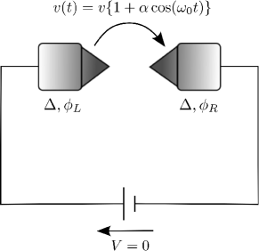
Figure 1: Schematic representation of a Josephson junction. We assume that the distance between the two leads is modulated periodically at a frequency $\omega_{0}$. This induces a weak modulation of the quantum hopping matrix element $v(t)$.

It consists of two bulk superconductors, characterized by a BCS gap $\Delta$, connected by a junction whose dimensions are assumed much smaller than the superconducting coherence length. This model can describe, for example, the contact between a STM superconducting tip and a bulk superconductor, or a quantum point contact in break junctions Della Rocca et al. (2007). The same model can also describe a quite different system: a suspended carbon nanotube between superconductors in the Fabry-Perot regime for a transparent barrier Kong et al. (2001). Different groups have realized suspended carbon nanotubes with good mechanical properties Lassagne et al. (2009); Steele et al. (2009). Also transparent contacts between superconductors and nanotubes forming SQUIDs have been observed Cleuziou et al. (2006); Pillet et al. (2010). The motion of the nanotube induces a modulation of the gate potential seen by the nanotube and thus modulates the transparency of the electronic mode. Note also that the mechanical coupling considered here is different from the one investigated in Ref. Sonne et al. (2010) for a suspended carbon nanotube in presence of magnetic field.

We will assume that the phase difference between the left (L) and right (R) superconducting leads, $\phi=\phi_{L}-\phi_{R}$ is time independent, i.e. there is no voltage drop at the junction. We consider the case of a single-channel superconducting point contact which can be described, for instance, by the following tight-binding Hamiltonian Levy Yeyati et al. (1995) (we set the units $\hbar=e=k_{B}=1$)

$$\hat{H}(t)=\sum_{X=L,R}\hat{H}_{X}+\hat{V}_{EM}(t)\;.$$ (2)

Here $\hat{H}_{X=L,R}$ are the Hamiltonians of the isolated $X=L,R$ leads given by

$$\hat{H}_{X}(t)=\sum_{i\in X}\psi_{i}^{\dagger}\Delta\hat{\sigma}_{x}\psi_{i}+\sum_{<i,j>\in X}\big{\{}\psi_{i}^{\dagger}\hat{v}_{0}\psi_{j}+\mbox{H.c}\big{\}}\;,$$ (3)

where $\hat{v}_{0}$ is the hopping matrix between next-nearest-neighbor sites within the isolated $X=L,R$ superconductors. We use the standard notation for the Pauli matrices in Nambu space $\{\hat{\sigma}_{x},\hat{\sigma}_{y},\hat{\sigma}_{z}\}$. The second term in the r.h.s. of Eq. (2) describes the (time dependent) hopping between the leads defined as

$$\hat{V}_{EM}(t) = \psi_{L}^{\dagger}\hat{v}(t)\psi_{R}+\psi_{R}^{\dagger}\hat{v}^{\dagger}(t)\psi_{L}$$ (4)

$$\hat{v}(t) = v(t)\hat{\sigma}_{z}e^{i\phi\hat{\sigma}_{z}/2}\,.$$ (5)

Notice that by a standard choice of the gauge, we have included the superconducting phase difference into the hopping term $\hat{v}$.

We focus our study on the electromechanical (EM) properties of the junction. We assume that one of the leads is vibrating at a radial frequency $\omega_{0}$, thus modulating the hopping term between the left and the right lead. In the limit where the amplitude of the oscillations is small, the time-dependent hopping will be linearly modulated as

$$v(t)=v\big{\{}1+\alpha\cos(\omega_{0}t)\big{\}}\;,$$ (6)

where $\alpha\equiv a{(1/v)}{dv/dx}\ll 1$, with $x$ the displacement of the oscillating lead and $a$ the amplitude of oscillation. We will give estimations for $\alpha$ in Sec. IV.

For large amplitude oscillation a detailed microscopic model of electron transport is needed. The standard tunneling picture gives a simple exponential dependence of the hopping on the displacement $v(x)=v(x_{0})e^{-(x-x_{0})/\lambda}$ where $\lambda$ is the tunneling length. But this picture would be different for the suspended nanotube, where a linear dependence on the displacement is supposed to hold for large oscillation amplitudes. For this reason in this paper we concentrate on the linear displacement model, which demands only a single parameter ( $\alpha$ ) to describe the EM coupling.

In the present model, the vibrational state of the junction is considered as an external time-dependent perturbation, without its own dynamics . Before proceeding to determine the current from the microscopic Hamiltonian [Eq. (2)], we start the next section by deriving an expression for the Josephson current within the framework of an effective two-level Hamiltonian. We will see that in a certain range of parameters, such a model provides an accurate description of the electronic dynamics of the contact.

III dc Josephson current

III.1 Andreev Two-Level Model

In a single-channel superconducting junction, as the one described by Eq. (2), the equilibrium spectral density is characterized by the two ABSs $\left|+\right\rangle$ and $\left|-\right\rangle$ with energies given in Eq. (1). In terms of the hopping [Eq. (5)], the transmission factor $\tau$ of the junction is defined as

$$\tau=\frac{4\beta}{(1+\beta)^{2}}\;,$$ (7)

where $\beta=(v/v_{0})^{2}$ is the ratio between the tunnel hopping amplitude and the electrode bandwidth $v_{0}$. In the equilibrium case, the dc current is carried exclusively by the ABSs and can be written as the sum of two opposite contributions Beenakker (1991)

$$I_{DC}^{(0)} = I_{-}n_{-}+I_{+}n_{+}\,,$$ (8)

$$I_{-} = -I_{+}=-2\frac{\partial}{\partial\phi}\omega_{A}=\frac{\Delta^{2}\tau\sin(\phi)}{2\omega_{A}}\;,$$ (9)

where $n_{\pm}$ is the occupation of the $\left|\pm\right\rangle$ ABSs which is given by the Fermi distribution function $f(\pm\omega_{A})$. Thus, in the finite temperature $T$ case one finally obtains the well known expression for the Josephson current (see Appendix)

$$I_{DC}^{(0)}(\phi)=\frac{\Delta^{2}\tau\sin(\phi)}{2\omega_{A}}\tanh(\frac{\omega_{A}}{2T})\,.$$ (10)

In the limit of zero temperature, only the negative ABS ($\left|-\right\rangle$) is populated, and contributes positively to the current in Eq. (10). At finite temperature $T$, the positive ABS ($\left|+\right\rangle$) gets populated due to the thermal smearing of the Fermi distribution and, according to Eq. (8) contributes negatively to the Josephson current.

Now let us consider the perturbation originated by the mechanical oscillations. If the frequency and amplitude of the perturbation are sufficiently small, one can still describe the current as the contribution of the two ABSs. In this case it is convenient to work with an effective two-level model Hamiltonian similar to the one derived in Refs. Zazunov et al. (2003, 2005) from the microscopic Hamiltonian Eq. (2). The main difference between the problem at hand and that considered in Refs. Zazunov et al. (2003, 2005) is that the time-dependent parameter is not the superconducting phase, but the transparency of the junction. Adapting the method to our problem, it gives the following effective time-dependent Hamiltonian for $d\tau/dt\ll\Delta/\hbar$:

$$\hat{h}(t)=\Delta\cos\frac{\phi}{2}\hat{\sigma}_{z}+\Delta\sqrt{1-\tau(t)}\sin\frac{\phi}{2}\hat{\sigma}_{y}\;.$$ (11)

This Hamiltonian is written in the ballistic basis of right and left moving electrons that is the eigenbasis in the perfectly transmitting case ($\tau=1$). However, it is more convenient to write the two-level Hamiltonian in the instantaneous Andreev basis Bergeret et al. (2011). For that sake, one performs a time-dependent unitary transformation $\hat{H}=\hat{U}^{\dagger}\hat{h}\hat{U}-i\hat{U}^{\dagger}d\hat{U}/dt$, where $\hat{U}(t)=e^{-i\hat{\sigma}_{z}\frac{\pi}{4}}e^{-i\theta(t)\hat{\sigma}_{y}}$ and $\theta(t)=(1/2)\arctan[\sqrt{1-\tau(t)}\tan\phi/2]$. The two-level Hamiltonian in the instantaneous Andreev basis is then given by

$$\hat{H}_{A}=\omega_{A}\hat{\sigma}_{z}+\frac{1}{8}\frac{d\tau}{dt}\frac{1}{\sqrt{1-\tau(t)}}\frac{\sin\phi}{1-\tau(t)\sin^{2}(\phi/2)}\hat{\sigma}_{y}\,.$$ (12)

The off-diagonal terms describe the coupling between the Andreev levels due to the EM oscillations. The current operator written in the same basis reads

$$\hat{I}_{A}=2\frac{\partial\omega_{A}}{\partial\phi}\hat{\sigma}_{z}+\frac{\Delta^{2}\sqrt{1-\tau(t)}}{\omega_{A}}\hat{\sigma}_{x}\;.$$ (13)

We consider here the time-dependent transmission determined by expressions Eqs. (6) and (7) which in a linear approximation with respect to the amplitude $\alpha$ is

$$\tau(t)\approx\tau+2\tau\sqrt{1-\tau}\alpha\cos(\omega_{0}t)\,.$$ (14)

In order to avoid unphysical values of $\tau$ larger than one one has to impose $\alpha<\sqrt{1-\tau}/2\tau$. More over in the particularly interesting case of very transparent channel, the linear term of Eq. (14) vanishes and it would be necessary to consider the quadratic one. Thus, for ($\tau\rightarrow 1$) comparison between the linear and quadratic term imposes the condition $\alpha\ll 2\sqrt{1-\tau}$.

We can now apply the method developed in Ref. Bergeret et al. (2011) to obtain time-averaged quantities like the current and the level population close to the first resonance, i.e. $\omega_{0}\approx 2\omega_{A}$. Within the rotating-wave approximation and for one-phonon assisted processes we obtain for the dc current

$$I_{DC}\approx I_{DC}^{(0)}\left[1-\frac{\Omega_{R}^{2}}{(2\omega_{A}-\omega_{0})^{2}+\Omega_{R}^{2}}\right]\,,$$ (15)

where the Rabi frequency

$$\Omega_{R}=\alpha\tau\sin(\phi)\omega_{0}\Delta^{2}/(2\omega_{A})^{2}$$ (16)

is proportional to the coupling strength $\alpha$. Notice that at the resonance, the dc current vanishes. This is due to the fact that when $\omega_{0}=2\omega_{A}$, resonant transitions between the Andreev levels take place and both levels will be on average equally populated. According to Eq. (8), this leads to a decrease of the dc current, which vanishes exactly at the resonance. The width of the resonance as given by Eq. (16) is proportional to the amplitude $\alpha$ of the oscillation. Thus, in principle by measuring the CPR one could determine both the amplitude and frequency of the contact oscillation as given by Eqs. (15) and (16). Finally, the time averaged population of the upper and lower Andreev states are given by

$$n_{-} = 1-\frac{1}{2}\frac{\Omega_{R}^{2}}{(2\omega_{A}-\omega_{0})^{2}+\Omega_{R}^{2}}\,,$$ (17)

$$n_{+} = \frac{1}{2}\frac{\Omega_{R}^{2}}{(2\omega_{A}-\omega_{0})^{2}+\Omega_{R}^{2}}\,.$$ (18)

These results are particularly simple and transparent, but they rely on different approximations. In the following section we will thus perform a fully microscopic calculation in order to check their validity. The method used does not need a hypothesis on the slowness of the mechanical frequency nor on the amplitude of the oscillations ($\alpha$) and keeps the full description of the electronic system. The approach allows us to take into account the effect of the continuum spectrum and in particular will remove the limitation on $\alpha\ll\sqrt{1-\tau}$. We will see that the largest deviations are exactly where higher orders of $\alpha$ become important ($\alpha>\sqrt{1-\tau}$) and when the resonant $\phi$ is close to $\pi$.

III.2 Nambu-Keldysh Green function method

In the preceding section we have determined the dc Josephson current from an effective two-level model. In this section we introduce a numerical method that allows us to compute exactly the dc Josephson current in the presence of EM coupling from the microscopic model introduced in Sec. II. From our results, we will able to verify the range of validity of Eqs. (15) and (16), and to obtain the current out of that range. The method is based on the computation of the Nambu-Keldysh Green functions (GFs) for the fermionic fields of the Hamiltonian  (2). These are defined as

$$\hat{G}_{XX^{\prime}}^{\alpha\beta}(t,t^{\prime})=-i\Big{\langle}T_{c}\psi^{\phantom{{\dagger}}}_{X}(t)\psi_{X^{\prime}}^{{\dagger}}(t^{\prime})\Big{\rangle}\,,$$ (19)

where $T_{c}$ means time ordering along the Keldysh contour, $\alpha,\beta=\pm$ denote the Keldysh branches, and $X,X^{\prime}=L,R$ stand for electrode indexes. From charge conservation at the L-R interface, one obtains the expression of the mean current crossing the junction at time $t$ in terms of the GFs

$$I(t)=\mbox{tr}\Big{\{}\hat{\sigma}_{z}\big{[}\hat{v}(t)\hat{G}_{RL}^{+-}(t,t)-\hat{v}^{\dagger}(t)\hat{G}_{LR}^{+-}(t,t)\big{]}\Big{\}}\,.$$ (20)

It is convenient to rewrite the Hamiltonian [Eq. (2)] as the sum of an unperturbed part plus the time-dependent perturbation

$$\hat{H}=\hat{H}_{0}+\hat{V}(t)\;,$$ (21)

where

$$\hat{H}_{0} = \sum_{X=L,R}\hat{H}_{X}+v\hat{W}_{T}\,,$$ (22)

$$\hat{V}(t) = \alpha v\cos(\omega_{0}t)\hat{W}_{T}\,,$$ (23)

and

$$\hat{W}_{T}=\psi_{L}^{\dagger}\hat{\sigma}_{z}e^{i\phi\hat{\sigma}_{z}/2}\psi_{R}+\psi_{R}^{\dagger}\hat{\sigma}_{z}e^{-i\phi\hat{\sigma}_{z}/2}\psi_{L}\,.$$ (24)

The corresponding Dyson equation is shown diagrammatically in Fig. 2.

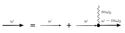
Figure 2: Schematic representation of the Dyson equation [Eq. (LABEL:dyson)] for the Green function in the Electrode-Nambu-Keldysh-Floquet space. The thick (thin) lines represent the Green functions in the vibrating (nonvibrating) case, while the wavy line represents the external time-dependent perturbation.

The thin lines represent the unperturbed Green’s functions, i.e., those associated to $\hat{H}_{0}$, while the thick lines are the exact GFs which take into account the external time-dependent perturbation represented by a wavy line. Due to the time periodicity of the Hamiltonian one can write the GFs in Floquet representation and the corresponding current operator as a Fourier series

$$\hat{G}_{XX^{\prime}}^{\alpha\beta}(t,t^{\prime})=\sum_{n}e^{-in\omega_{0}t^{\prime}}\int\frac{d\omega}{2\pi}e^{-i\omega(t-t^{\prime})}\hat{G}_{XX^{\prime};n}^{\alpha\beta}(\omega)\,,$$

(25)

$$I(t)=\sum_{n}e^{-in\omega_{0}t}I_{n}\,.$$ (26)

We are interested in the dc component ($n=0$) of the mean current given by

$$I_{DC}(\phi)=$$

$$\sum_{m}\int\frac{d\omega}{2\pi}\mbox{tr}\Big{\{}\hat{\sigma}_{z}\big{[}\hat{v}_{m0}\hat{G}_{RL;0m}^{+-}(\omega)-\hat{v}^{\dagger}_{m0}\hat{G}_{LR;0m}^{+-}(\omega)\big{]}\Big{\}}\,,$$

where the hopping matrix $\hat{v}$ in the Floquet space is defined as

$$\hat{v}_{m0}=\hat{v}\big{\{}\delta_{m,0}+\frac{\alpha}{2}\delta_{m,\mp 1}\big{\}}\,.$$ (28)

The Dyson equation in the frequency representation is then given by (cf. Fig. 2)

$$\hat{G}_{XX^{\prime};n}^{\alpha\beta}(\omega)=\hat{g}_{XX^{\prime}}^{\alpha\beta}(\omega)\delta_{n,0}+$$

$$\sum_{X_{1},\alpha_{1},m}\left[\hat{g}_{XX_{1}}^{\alpha\alpha_{1}}(\omega)\hat{V}_{X_{1}\overline{X}_{1};m}^{\alpha_{1}}\hat{G}_{\overline{X}_{1}X^{\prime};n-m}^{\alpha_{1}\beta}(\omega-m\omega_{0})\right]\;.$$

Here the self-energy term is given by

$$\hat{V}_{X_{1}\overline{X}_{1};m}^{\alpha_{1}}=\alpha_{1}\big{(}\frac{\alpha}{2}\big{)}\hat{v}_{X_{1}\overline{X}_{1}}\delta_{m;\pm 1}\,,$$ (30)

and the expressions for the free propagators $\hat{g}_{XX^{\prime}}^{\alpha\beta}(\omega)$ in the absence of vibrations ($\alpha=0$) are given in the Appendix.

In the case $\alpha\neq 0$, however, the GFs $\hat{G}_{XX^{\prime};n}^{\alpha\beta}(\omega)$ can only be found numerically by solving the Dyson equation (LABEL:dyson). The latter constitutes a linear system in the Electrode-Nambu-Keldysh-Floquet space of dimension $2\times 2\times 2\times(2N_{ph}+1)$ and is solved by exact numerical inversion. The maximum number of vibrational quanta in the system $N_{ph}$ is increased until convergence of the solution is found .

IV Discussion of the results

Following the procedure described in the previous section we present in Fig. 3 the numerical results obtained for the dc Josephson current in the presence of the EM interaction for a highly transmitting junction ($\tau=0.98$). The dark dotted line represents the dc current $I_{DC}^{(0)}(\phi)$ obtained in absence of vibrations ($\alpha=0$) as it is given by Eq. (10). For $\omega_{0}=0.4\Delta$ and $\alpha=0.04$ the dashed and solid lines show the results of the two-level model [Eq. (15)] and the full numerical solution, respectively.

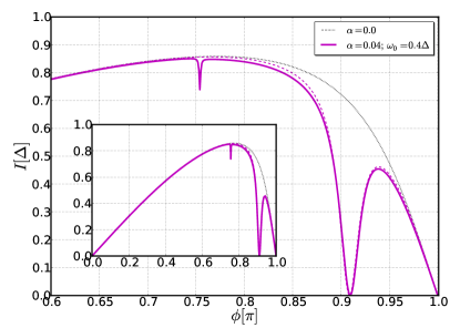
Figure 3: Josephson current for $\omega_{0}=0.4\Delta$, $\tau=0.98$, $\alpha=0.04$, $T=0\mbox{ K}$, and $\eta=0.001\Delta$ ($\eta$ is the inverse of the relaxation time of the superconductor as defined in the Appendix). Plain (dashed) curves correspond to the full numerical (analytical) calculations. Dotted curve: current in the case of vanishing $\alpha$. Inset: Same plot on a larger scale.

As anticipated before, the EM coupling induces an antiresonance on the dc Josephson current when the condition $\omega_{0}=2\omega_{A}$ is fulfilled, namely when the phase difference between L and R superconductors reaches the critical value

$$\phi_{res}=2\arcsin{\sqrt{\frac{1}{\tau}\big{[}1-(\frac{\omega_{0}}{2\Delta})^{2}\big{]}}}\,.$$ (31)

The signature of such a modulation is the presence of dips in the current-phase relation, the position of which provides a measure of the vibrational frequency $\omega_{0}$ through the resonance condition Eq. (31). The width of the dip is proportional to the coupling $\alpha$ between the nano-resonator and the vibrational mode of the junction being excited. It is well approximated by the expression (16). The numerics show some additional dips in the CPR that are associated with higher-order transitions. Such processes which are obviously absent from Eq. (15) could be incorporated by extending the analytical calculation to the next leading orders in powers of $\alpha$ (see Refs.Bergeret et al. (2010, 2011)). According to the upper panel of Fig. 4, the resonance dip is accurately approximated both in position and width by the Eq. (15). The discrepancy between the simplified two-level model and the full numerical calculation becomes visible when increasing the value of $\alpha$. This deviation is due to the fact that for large enough values of $\alpha$ the condition $\alpha<\sqrt{1-\tau}$ is not satisfied. In the particular case of the upper panel of Fig. 4, $\alpha=0.01-0.025$, $\tau=0.999$ and $\omega_{0}=0.1\Delta$. Therefore the analytical result is valid as far as $\alpha<0.03$. For larger values of $\alpha$, Eq. (15) is no longer valid and one has to resort to numerical results. These are shown in the lower panel of Fig. 4, where $\alpha=0.04-0.1$. The parameters used in Fig. 4 correspond to a high-frequency oscillator $\omega_{0}/2\pi=1\mbox{ GHz}$ and a superconductor with a small superconducting gap $\Delta\approx 0.04\mbox{ meV}$. Suspended carbon nanotubes between two superconductors seem to be good candidates to reach this regime. For instance, the resonant frequency for the fundamental mode of such a vibrating nanotube was reported in Ref. Hüttel et al. (2010) to be in the range of 500 MHz. In Ref. Herrmann et al. (2010) a carbon nanotube was connected to a superconducting Al/Pd bilayer electrode with a BCS gap of 0.08 meV which is in the range of our estimation.

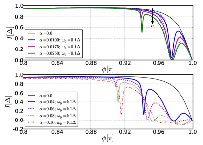
Figure 4: Upper panel: Josephson current for the cases of EM coupling $\alpha=0.01,0.0175,0.025$ (within the range of validity of the analytic model). Plain (dashed) curves correspond to the full numerical (analytical) calculation. The arrow is denoting the direction of increasing values of $\alpha$. Lower panel: Josephson current for the cases of larger EM coupling $\alpha=0.04,0.06,0.08,0.1$, as obtained from the full numerical calculation. Common to all curves: $\tau=0.999$, $\omega_{0}=0.1\Delta$, $\eta=0.001\Delta$ and $T=0\mbox{ K}$. Topmost curve: current in the case $\alpha=0.0$.

As mentioned above some differences between the numerical results and the analytical one emerge for $\phi$ close to $\pi$ that become more pronounced when increasing the value of the coupling strength $\alpha$, as shown in the lower panel of Fig. 4, for which $\alpha=0.04-0.1$. Notice that in this regime the exact numerical calculation predicts a change of the current sign close to $\phi=\pi$ due to higher order processes.

The results presented show that measuring the current phase relation in a Josephson junction coupled to a mechanical oscillator can allow the detection of its periodic oscillation (for example when the oscillator is driven by an external force). We found that the CPR displays sharp dips when the resonance condition $\omega_{0}=2\omega_{A}$ is met. According to Eq. (1) for $\tau\rightarrow 1$ and $\omega_{A}(\phi=\pi)\rightarrow 0$, one can in principle always satisfy the resonant condition. In reality this can be difficult, since it requires $\tau$ being very near to one and $\Delta$ for standard superconductors is much larger than the typical mechanical frequency. This problem can be solved by using superconducting alloys with smaller gap, or by introducing a magnetic field in order to reduce $\Delta$ to a value which is slightly larger than the mechanical resonance. Then the fine tuning of the resonance with the phase bias can be possible.

The second crucial parameter in order to observe this effect is the coupling constant $\alpha$. A reasonable estimate of the order of magnitude of $\alpha$ can be obtained by considering the experiment of Ref. Flowers-Jacobs et al. (2007), which was performed on a driven nanomechanical oscillator in its normal metallic state. The authors of Ref. Flowers-Jacobs et al. (2007) estimate the resistance dependence on the displacement to be $(1/R)dR/dx\sim 0.1{\rm nm}^{-1}$, with a typical displacement in the driven case of the order of a nm. Thus a very crude estimate of the order of magnitude of $\alpha$ is $0.1$, that is a quite strong coupling. Remarkably, for a suspended carbon nanotube in the Fabry-Perot regime we find a similar order of magnitude. This can be estimated by using the responsivity of the transparency to an external change of gate voltage from Ref. Kong et al. (2001) and $(1/C_{g})dC_{g}/dx\approx 1/d$, where $C_{g}$ is the gate capacitance, and $d$ is the distance of the nanotube from the gate. It is clear that at this level these are only crude estimates of the order of magnitude of $\alpha$, but the result is encouraging.

In principle one could also detect thermal motion of the mechanical oscillator with this method if the quality factor ($Q$) of the mechanical oscillator is sufficiently large As a matter of facts, the thermal motion can be seen as a sequence of periodic oscillations with a coherence time given by $Q/\omega_{0}$. Averaging the current over a time much longer than this time corresponds to averaging the current obtained above over different values of the amplitudes of oscillation (and thus of $\alpha$). One thus expects also in this case a dip in the CPR, but with a width that is controlled by the average of $\alpha$. In the case of Ref. Flowers-Jacobs et al. (2007) this motion is tiny and gives that on average $\alpha\approx 10^{-4}$. This gives an extremely sharp dip, and thus its observation is subject to a very accurate detection of the CPR.

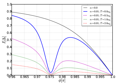
Figure 5: Josephson current in the finite temperature case $T=0.0,0.5,1.0,2.0\omega_{0}$, as obtained from the full numerical calculation. Parameters of the plot: $\tau=0.999$, $\omega_{0}=0.1\Delta$, $\alpha=0.01$ and $\eta=0.001\Delta$. Topmost curve: current in the case $\alpha=0.0$.

All the results presented so far are for the zero temperature limit. In the case of finite temperature, the coupling of the quantum point contact to the mechanical oscillator may lead to enhancement of the supercurrent as was discussed in the context of a microwave field Bergeret et al. (2010, 2011). The enhancement of the current is due to inelastic processes which promote particles from the continuum spectrum ($\omega<-\Delta$) to the lower ABS. This phenomenon (not shown here) is an analog to the superconducting stimulation by acoustic waves in bulk materials discussed by Eliashberg and Ivlev in 1986 Eliashberg and Ivlev (1986).

But more important to the efficiency of this device as a detector is the fact that thermal fluctuations can prevent the observation of the mechanical oscillations. For temperatures of the order of and larger than $\omega_{0}=2\omega_{A}$, the thermal occupation of the two-level system tends to the value $1/2$: $n_{\pm}=f(\pm\omega_{0}/2)\approx 1/2\mp\omega_{0}/(8T)+o(\omega_{0}^{3})$. This effect will reduce the overall value of the Josephson current; nevertheless by the exact numerical solution, we find that a signal is still visible till moderately high temperatures. As it is shown in Fig. 5, for $T=0.5-2\omega_{0}$ the CPRs maintain a local minimum at the resonance. The position of the dip is independent of the temperature [cf. Eq. (31)] while it widens for higher temperatures.

One should emphasize that the back action of the Josephson junction on the mechanical oscillator is neglected in the present work. The establishment of an effective two-level model for the Josephson junction description opens the way to considering the full dynamics of the two systems coupled. At this stage, we can evaluate the ratio of the average of the back-action force $\langle\hat{F}_{ba}(t)\rangle=-\langle{\partial\hat{h}(t)}/{\partial x}\rangle$ to the elastic force $F_{el}=-m\omega_{0}^{2}x$. We find that ${\langle\hat{F}_{ba}(t)\rangle}/{F_{el}}\approx{3\Delta}/{4m\omega_{0}^{2}\lambda^{2}}$, where we introduced the characteristic length $\lambda=v/(dv/dx)$. Interestingly, this ratio is independent of the amplitude of the oscillations. For a single wall carbon nanotube of mass $m\approx 10^{-21}\mbox{ kg}$ that oscillates at the frequency $\omega_{0}/{2\pi}=1\mbox{ GHz}$, we roughly estimate this ratio to be in the range $10^{-4}-10^{-6}$ . Although very small, this back action may lead to interesting effects as the cooling effect of the mechanical degree of freedom in the presence of an external magnetic field Sonne et al. (2010). Note also that we have safely neglected the effects of Coulomb blockade on the mechanical oscillation Pauget et al. (2008); Pistolesi and Labarthe (2007) since the interesting region for this device is the very transparent case.

V Conclusions

In conclusion we have shown the possibility of detecting ultrafast oscillations of a nano-scale Josephson junction by analyzing its dc current-phase characteristics. In the high transmission regime $\tau\approx 1$, the onset of electromechanical coupling results in the appearance of dips in the $I_{DC}(\phi)$ characteristics for precise values of the phase difference $\phi$. The location of those dips provides a new way to measure the vibrational frequency $\omega_{0}$ of the oscillator, and their width is directly proportional to the EM coupling strength $\alpha$. If the latter is sufficiently small, we have derived an effective two-level Hamiltonian [Eq. (12)] which describes quite accurately the dynamics of the contact in the presence of an EM perturbation. Our results provide a new way of characterizing the motion at the nanoscale.

Appendix : Free Green functions

Here we determine the GFs of the nonvibrating Josephson junction ($\alpha=0$). We first consider the isolated Right electrode described by the time-independent Hamiltonian (Eq. (3)). The retarded (R) and advanced (A) surface Green functions of such a system can be found analytically by making use of the periodicity of the Hamiltonian when writing its Dyson equation

$$\hat{g}_{R}^{\eta=R(A)}(\omega)=\Big{\{}\omega_{\eta}-\Delta\hat{\sigma}_{x}-\hat{v}_{0}\hat{g}_{R}^{\eta=R(A)}(\omega)\hat{v}^{\dagger}_{0}\Big{\}}^{-1}$$ (32)

where $\omega_{\eta}=\omega+i\eta$. The small imaginary part describes inelastic scattering in the leads within the relaxation time approximation and is the smallest energy scale of the problem. In the small gap limit ($\Delta,\omega<<2|v_{0}|$, $v_{0}$ is the electrode bandwidth), one finds for the solution of Eq.32

$$\hat{g}_{S}^{\eta=R(A)}(\omega)=N_{\eta}(\omega)\Big{\{}\omega_{\eta}+\Delta\hat{\sigma}_{x}\Big{\}}$$ (33)

where $N_{\eta}(\omega)=-\frac{1}{v_{0}}\Big{\{}\frac{\theta(|\Delta|-|\omega|)}{\sqrt{|\Delta|^{2}-\omega_{\eta}^{2}}}+i\eta\mbox{sign}(\omega)\frac{\theta(|\omega|-|\Delta|)}{\sqrt{\omega_{\eta}^{2}-|\Delta|^{2}}}\Big{\}}$.

We connect now the R-lead to the L-lead through the time-independent part of the tunnel Hamiltonian (Eq.4). The Dyson equations for the retarded (advanced) GFs of the entire nano-junction read

$$\hat{G}_{R}^{\eta=R(A)}(\omega) = \frac{1}{\big{(}\hat{g}_{R}^{\eta=R(A)}\big{)}^{-1}(\omega)-\hat{v}^{\dagger}\hat{g}_{L}^{\eta=R(A)}(\omega)\hat{v}}$$ (34)

$$\hat{G}_{LR}^{\eta=R(A)}(\omega) = \hat{g}_{L}^{\eta=R(A)}(\omega)\hat{v}\hat{G}_{R}^{\eta=R(A)}(\omega)$$ (35)

Eqs.(34-35) can be solved analytically and provide the expressions for the unperturbed GFs used in Eq. (LABEL:dyson)

$$\hat{G}_{R}^{\eta=R,A}(\omega) = \frac{g_{\eta}(\omega)}{|v_{0}|(1+\beta)(\omega_{\eta}^{2}-\omega_{A}^{2})}\left[\begin{array}[]{cc}\omega_{\eta}&\underline{\omega}_{A}^{*}\\ \underline{\omega}_{A}&\omega_{\eta}\end{array}\right]$$ (38)

$$\hat{G}_{LR}^{\eta=R,A}(\omega) = \frac{\beta}{|v|(1+\beta)(\omega_{\eta}^{2}-\omega_{A}^{2})}\left[\begin{array}[]{cc}a(\phi)&-b(-\phi)\\ b(\phi)&-a(-\phi)\end{array}\right]$$ (41)

$$a(\phi) = e^{i\phi/2}\omega_{\eta}^{2}-e^{-i\phi/2}\underline{\omega}_{A}\Delta$$ (42)

$$b(\phi) = \omega_{\eta}(e^{i\phi/2}\Delta-e^{-\phi/2}\underline{\omega}_{A})$$ (43)

where we introduced the intermediate function $g_{\eta}(\omega)=\theta(|\Delta|-|\omega|)\sqrt{|\Delta|^{2}-\omega_{\eta}^{2}}-i\eta\mbox{sign}(\omega)\theta(|\omega|-|\Delta|)\sqrt{\omega_{\eta}^{2}-|\Delta|^{2}}$ and the complex number $\underline{\omega}_{A}=\Delta\frac{1+\beta e^{i\phi}}{1+\beta}$, the module of which is the Andreev bound state energy $\omega_{A}=\Delta\sqrt{1-\tau\sin^{2}(\phi/2)}$. The remaining components of the GFs are obtained by changing simultaneously left and right electrode indexes and the sign of the superconducting phase difference, i.e., $(L,\phi)\rightarrow(R,-\phi)$.

Finally, the non diagonal component of the Keldysh GFs can be found using the relation (valid at equilibrium only)

$$\hat{G}_{XX^{\prime}}^{+-}(\omega)=f(\omega)\big{\{}\hat{G}_{XX^{\prime}}^{A}(\omega)-\hat{G}_{XX^{\prime}}^{R}(\omega)\big{\}}\;,$$ (44)

where $f$ is the Fermi distribution function. From this equation one can compute the equilibrium Josephson current (Eq.10) by integrating the following expression

$$I_{DC}^{(0)}(\phi)=\int\frac{d\omega}{2\pi}\mbox{tr}\Big{\{}\hat{\sigma}_{z}\Big{[}\hat{v}\hat{G}_{RL}^{+-}(\omega)-\hat{v}^{\dagger}\hat{G}_{LR}^{+-}(\omega)\Big{]}\Big{\}}\,.$$ (45)

References

- O’Connell et al. (2010) A. D. O’Connell, M. Hofheinz, M. Ansmann, R. C. Bialczak, M. Lenander, E. Lucero, M. Neeley, D. Sank, H. Wang, M. Weides, et al., Nature 464, 697 (2010).
- Regal et al. (2008) C. A. Regal, J. D. Teufel, and K. W. Lehnert, Nature Physics 4, 555 (2008).
- Rocheleau et al. (2010) T. Rocheleau, T. Ndukum, C. Macklin, J. B. Hertzberg, A. A. Clerk, and K. C. Schwab, Nature 463, 72 (2010).
- Suh et al. (2009) J. Suh, M. LaHaye, P. Echternach, K. Schwab, and M. Roukes, Nano Lett. 10, 3990 (2009).
- Arcizet et al. (2006) O. Arcizet, P.-F. Cohadon, T. Briant, M. Pinard, and A. Heidmann, Nature 444, 71 (2006).
- Ding et al. (2010) L. Ding, C. Baker, P. Senellart, A. Lemaitre, S. Ducci, G. Leo, and I. Favero, Phys. Rev. Lett. 105, 263903 (2010).
- Aspelmeyer et al. (2010) M. Aspelmeyer, S. Gröblacher, K. Hammerer, and N. Kiesel, J. Opt. Soc. Am. B 27, A189 (2010).
- Lassagne et al. (2009) B. Lassagne, Y. Tarakanov, J. Kinaret, D. Garcia-Sanchez, and A. Bachtold, Science 325, 1107 (2009).
- Steele et al. (2009) G. Steele, A. Huettel, B. Witkamp, M. Poot, B. Meerwaldt, L. Kouwenhoven, and H. van der Zant, Science 325, 1103 (2009).
- Flowers-Jacobs et al. (2007) N. E. Flowers-Jacobs, D. R. Schmidt, and K. W. Lehnert, Phys. Rev. Lett. 98, 096804 (2007).
- Blencowe (2004) M. P. Blencowe, Phys. Rep. 395, 159 (2004).
- Bocko and Onofrio (1996) M. F. Bocko and R. Onofrio, Rev. Mod. Phys. 68, 755 (1996).
- Clerk and Girvin (2004) A. A. Clerk and S. M. Girvin, Phys. Rev. B 70, 121303 (2004).
- Naaman et al. (2001) O. Naaman, W. Teizer, and R. C. Dynes, Phys. Rev. Lett. 87, 097004 (2001).
- Della Rocca et al. (2007) M. L. Della Rocca, M. Chauvin, B. Huard, H. Pothier, D. Esteve, and C. Urbina, Phys. Rev. Lett. 99, 127005 (2007).
- Zgirski et al. (2011) M. Zgirski, L. Bretheau, Q. Le Masne, H. Pothier, D. Esteve, and C. Urbina, Phys. Rev. Lett. 106, 257003 (2011).
- Pillet et al. (2010) J.-D. Pillet, C. H. L. Quay, P. Morfin, C. Bena, A. Levy Yeyati, and P. Joyez, Nature Phys. 6, 965 (2010).
- Zhu et al. (2006) J.-X. Zhu, Z. Nussinov, and A. V. Balatsky, Phys. Rev. B 73, 064513 (2006).
- Fransson et al. (2008) J. Fransson, J.-X. Zhu, and A. V. Balatsky, Phys. Rev. Lett. 101, 067202 (2008).
- (20) A. Furusaki and M. Tsukada, Solid State Commun. 78, 299 (1991).
- Beenakker (1991) C. W. J. Beenakker, Phys. Rev. Lett. 67, 3836 (1991).
- Zazunov et al. (2003) A. Zazunov, V. S. Shumeiko, E. N. Bratus’, J. Lantz, and G. Wendin, Phys. Rev. Lett. 90, 087003 (2003).
- Clerk et al. (2010) A. A. Clerk, M. H. Devoret, S. M. Girvin, F. Marquardt, and R. J. Schoelkopf, Rev. Mod. Phys. 82, 1155 (2010).
- Bergeret et al. (2010) F. S. Bergeret, P. Virtanen, T. T. Heikkilä, and J. C. Cuevas, Phys. Rev. Lett. 105, 117001 (2010).
- Bergeret et al. (2011) F. S. Bergeret, P. Virtanen, A. Ozaeta, T. T. Heikkilä, and J. C. Cuevas, Phys. Rev. B 84, 054504 (2011).
- Kong et al. (2001) J. Kong, E. Yenilmez, T. W. Tombler, W. Kim, H. Dai, R. B. Laughlin, L. Liu, C. S. Jayanthi, and S. Y. Wu, Phys. Rev. Lett. 87, 106801 (2001).
- Cleuziou et al. (2006) J.-P. Cleuziou, W. Wernsdorfer, V. Bouchiat, T. Ondarçuhu1, and M. Monthioux, Nature Nanotech. 1, 53 (2006).
- Sonne et al. (2010) G. Sonne, M. E. Peña Aza, L. Y. Gorelik, R. I. Shekhter, and M. Jonson, Phys. Rev. Lett. 104, 226802 (2010).
- Levy Yeyati et al. (1995) A. Levy Yeyati, A. Martín-Rodero, and F. J. García-Vidal, Phys. Rev. B 51, 3743 (1995).
- Zazunov et al. (2005) A. Zazunov, V. S. Shumeiko, G. Wendin, and E. N. Bratus’, Phys. Rev. B 71, 214505 (2005).
- Hüttel et al. (2010) A. K. Hüttel, H. B. Meerwaldt, G. A. Steele, M. Poot, B. Witkamp, L. P. Kouwenhoven, and H. S. J. van der Zant, physica status solidi (b) 247, 2974 (2010), ISSN 1521-3951.
- Herrmann et al. (2010) L. G. Herrmann, F. Portier, P. Roche, A. L. Yeyati, T. Kontos, and C. Strunk, Phys. Rev. Lett. 104, 026801 (2010).
- Eliashberg and Ivlev (1986) G. M. Eliashberg and B. I. Ivlev, edited by D. N. Langeberg and A. I. Larkin (North-Holland, Amsterdam) (1986).
- Pauget et al. (2008) N. Pauget, F. Pistolesi, and M. Houzet, Phys. Rev. B 77, 235318 (2008).
- Pistolesi and Labarthe (2007) F. Pistolesi and S. Labarthe, Phys. Rev. B 76, 165317 (2007).