Intersection of two TASEP traffic lanes
with frozen shuffle update
XXX

Abstract

Motivated by interest in pedestrian traffic we study two lanes (one-dimensional lattices) of length $L$ that intersect at a single site. Each lane is modeled by a TASEP (Totally Asymmetric Exclusion Process). The particles enter and leave lane $\sigma$ (where $\sigma=1,2$) with probabilities $\alpha_{\sigma}$ and $\beta_{\sigma}$, respectively. We employ the ‘frozen shuffle’ update introduced in earlier work [C. Appert-Rolland et al, J. Stat. Mech. (2011) P07009], in which the particle positions are updated in a fixed random order. We find analytically that each lane may be in a ‘free flow’ or in a ‘jammed’ state. Hence the phase diagram in the domain $0\leq\alpha_{1},\alpha_{2}\leq 1$ consists of four regions with boundaries depending on $\beta_{1}$ and $\beta_{2}$. The regions meet in a single point on the diagonal of the domain. Our analytical predictions for the phase boundaries as well as for the currents and densities in each phase are confirmed by Monte Carlo simulations.

Keywords: pedestrian traffic, exclusion process, shuffle update

LPT Orsay 11/xx

1 Introduction

P edestrian motion has raised increasing interest in the past years, both from a practical and a theoretical point of view. Understanding the behavior of crowds or of waiting lines is still a challenge. Simplified models may help to understand the behavior of individuals and the resulting collective behavior in various settings. In a large class of models [1, 2] pedestrians are represented as hard core particles moving on a lattice according to certain rules of motion. One important ingredient of these rules is the type of update scheme that is employed. Actually the update scheme is an integral part of the model definition; changing the scheme may change the interpretation and the properties of the model [3].

In the past two types of updates have been used for pedestrians modeling: the random shuffle update [4, 5, 6, 7] which has been later replaced by the parallel update [8, 9]. In [10, 11] we have proposed a new update scheme for pedestrian modeling, the frozen shuffle update, that we shall use in this paper. Its characteristic feature is that during each time step all particles present in the system are updated in a fixed random sequence. Newly entering particles are inserted in this updating sequence and exiting particles are deleted from it according to a suitable algorithm. Frozen shuffle update was inspired originally by the need for a physically motivated rule of priority in cases where more than one particle attempts to hop simultaneously towards the same target site. This update has the additional advantages that it is easily implemented in a Monte Carlo simulation and lends itself well to analytic study.

The consequences of frozen shuffle update were worked out previously for the case of a one-dimensional totally asymmetric exclusion process (TASEP) both on a ring [10] and with open boundary conditions [11]. On a finite one-dimensional lattice with open boundaries two parameters $\alpha$ and $\beta$ describe the probabilities for particles to enter the system at one end and to leave it at the other end. In this case the particle density $\rho$ and the current $J$ must be determined as a function of $\alpha$ and $\beta$. For varying $\alpha$ there appears to be a critical point $\alpha=\beta$ between a ‘free flow’ and a ‘jammed’ state.

One of our purposes is to model pedestrian motion at the intersection of two corridors or two streets and to study how global structures emerge from local interactions. As a step toward this goal we study in the present paper a TASEP on two perpendicular traffic lanes, 1 and 2, that intersect at a single lattice site and whose entrance and exit parameters are $\alpha_{1},\alpha_{2},\beta_{1},$ and $\beta_{2}$. The main question is again to determine the stationary state currents ${J}_{1}$ and ${J}_{2}$ in this two lane system as a function of these four parameters. For each lane one may expect two possibilities, a free flow (F) or a jammed (J) state. We will study the phase diagram in the $\alpha_{1}\alpha_{2}$ plane for $0\leq\alpha_{1},\alpha_{2}\leq 1$, considering $\beta_{1}$ and $\beta_{2}$ as fixed parameters. Indeed we find a division of this square domain into four different regions denoted FF, FJ, JF, and JJ, and separated by phase boundaries for which we obtain analytic expressions.

In earlier analytic work [10] on the frozen shuffle update the concept of a ‘platoon’ was introduced. It will again play a role in this paper. We will, moreover, point out here a new phenomenon, to be called the ‘pairing mechanism’, which is operative at the intersection. It says, basically, that when both lanes are in the jammed state, a platoon crossing the intersection on lane $1$ is always accompanied by a platoon crossing the intersection on lane $2$. This mechanism, which is an unintended consequence of the rules of motion, will enable us to extend the theoretical analysis from the single lane to the case of two intersecting lanes.

This article is organized as follows. In section 2 we define the exact rules of motion of this intersecting lane model and recall the concept of a ‘platoon’. In a short section 3 we recall the single lane results that will be needed again here. In subsection 4.1 we argue that the FF phase, expected to exist at low entrance rates, cannot extend beyond a certain curve in the $\alpha_{1}\alpha_{2}$ plane. In subsection 4.2 we show that if a JJ phase exists, the exiting flow must obey a pairing mechanism. Exploiting this mechanism we determine in subsections 4.3 and 4.4 the phase boundaries of the intermediate FJ/JF states with the JJ and FF states, respectively, and thereby confirm the existence of all four possible phases. We obtain analytical expressions for the currents in both lanes in each of the four phases. In subsection 4.5 we consider various limits in the $\alpha_{1}\alpha_{2}$ domain. In section 5 we derive expressions for the particle densities which, in contrast to the currents, are discontinuous at the phase boundaries. In section 6 we present a few simulation results. The data for the current fall right onto the theoretical curves, whereas the density data show finite size effects similar to those encountered and explained in the single lane case [11]. Section 7 is our conclusion.

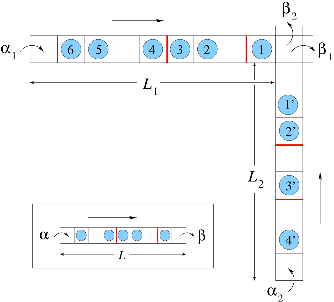
Figure 1: The two lane configuration studied in this work. The arrows indicate the flow direction. A heavy (red) bar indicates an end-of-platoon. The entrance probabilities are $\alpha_{1}$ and $\alpha_{2}$, the exit probabilities from the intersection site are $\beta_{1}$ and $\beta_{2}$.   Inset: the single lane with parameters $\alpha$ and $\beta$ studied in reference [11].

2 Rules of the motion

2.1 Rules

We consider the geometry shown in figure 1, consisting of two perpendicular one-dimensional lattices (or: lanes) labeled by an index $\sigma=1,2$. Hard core particles may move to the right on lane 1 and upward on lane 2. The lanes have $L_{1}$ and $L_{2}$ sites, respectively, plus a common intersection site. Particles enter at the two extremal sites and exit when leaving the intersection site. In our analytical treatment we shall imagine that both $L_{\sigma}$ tend to infinity. As usual in critical phenomena, finite size effects will be important only in the critical region. In practice, our infinite system results apply as soon as the $L_{\sigma}$ are large compared to the boundary layers near the entrance or exit.

A particle $i$, when entering the system, is assigned, in a way discussed below, a phase $\tau_{i}\in[0,1)$ which it keeps as a fixed attribute until it exits the system. Although the time $t$ is continuous, the time evolution is best described in terms of integer time steps $s=1,2,3,\ldots$. During each time step the particles are visited in the order of increasing phases and their positions are updated according to the following rules.

General rule.   When a lane 1 (lane 2) particle is updated, it moves one lattice distance to the right (upward) if the target site is empty, and does not move if the target site is occupied. The update of particle $i$ during the $s$th time step is considered to take place at the exact moment $t=s+\tau_{i}$ .

The general rule must be supplemented by two special rules for entering and exiting particles.

Exiting rule.   A particle $i$ which at the beginning of the $s$th time step is on the intersection site, will at time $s+\tau_{i}$ leave the system with probability $\beta_{1}$ (or $\beta_{2}$) according to whether it has arrived through lane 1 (or lane 2). Once it leaves the intersection site, we do not consider it any longer: it has left the system.

Entering rule.   When the entrance site of lane $\sigma$ becomes vacant at time $t$, it will be occupied by a new particle, injected from outside, at a random time $t^{\prime}=t+T$. Here $T$ is drawn from the exponential distribution

$$P_{\sigma}(T)=a_{\sigma}\,{\rm e}^{-a_{\sigma}T},\qquad 0\leq T<\infty,$$ (2.1)

where the ‘entrance rate’ $a_{\sigma}>0$ is a model parameter.

Equivalent to $a_{\sigma}$ is the ‘entrance probability’ $\alpha_{\sigma}$ defined by

$$\alpha_{\sigma}=1-{\rm e}^{-a_{\sigma}},\qquad\sigma=1,2,$$ (2.2)

which is the conditional probability that the entrance site of lane $\sigma$ is occupied at time $t+1$ given that it was vacant at time $t$. Henceforth we will sometimes let $a_{\sigma}$ and $\alpha_{\sigma}$ occur in the same expression.

To see the motivation for the above entering rule, one may notice that each particle arrival on the entrance site (or, for that matter, on any other site) is followed by one unit of ‘dead time’ during which no new arrival on that site is possible. Subject to this dead time condition, the entering rule distributes the instants of arrival of the particles at the entrance site uniformly on the time axis .

2.2 Platoons

The phases $\tau_{i}$ may be regarded as quenched random variables. With the rules stated above the particle motion is deterministic apart from the stochastic phase assignment at the entrances and, when $\beta_{1}<1$ or $\beta_{2}<1$, the stochastic exits. As a consequence of the entering rule the phase $\tau^{\prime}$ of the newly injected particle is related to the phase $\tau$ of its predecessor in the same lane by

$$\tau^{\prime}=(\tau+T)\,{\rm mod}\,1.$$ (2.3)

It follows that there are correlations between the phases of successive particles in the same lane. Following a lane in the direction opposite to the particle flow, one may group the particles together into sequences of increasing phases, a phase decrease signaling the beginning of a new sequence. When particles constituting such an increasing phase sequence occupy consecutive sites, they are said to constitute a ‘platoon’. The average platoon length $\nu$ associated with an entrance probability $\alpha$ is given by [11]

$$\frac{1}{\nu(\alpha)}=1+\frac{1}{a}-\frac{1}{\alpha}\,.$$ (2.4)

where $\alpha\equiv 1-{\rm e}^{-a}$. This quantity will play an essential role in the analysis that follows.

3 Stationary states in a single lane

The single lane problem with boundary conditions $\alpha$ and $\beta$, shown in the inset of figure 1, has yielded [11] results some of which will again be needed here. First, we know that the entrance probability $\alpha$ (for large enough $\beta$) imposes a ‘free flow’ bulk state, that is, one in which all attempted moves are successful, which carries a current

$$J^{\rm F}(\alpha)=\frac{a}{1+a}\,.$$ (3.1)

Secondly, it was shown [11] that the exit probability $\beta$ (for large enough $\alpha$) imposes a jammed bulk state. This is a state in which all particles belong to platoons and successive platoons are separated by at most a single vacancy. The jammed state has an outgoing current

$$J^{\rm J}(\alpha,\beta)=\frac{\nu}{\frac{\nu}{\beta}+1}\,,$$ (3.2)

with $\nu$ determined by $\alpha$ through (2.4). This exit flow can be sustained if and only if the entering flow is sufficiently large, that is for $J^{\rm F}>J^{\rm J}$. The equality $J^{\rm F}(\alpha)=J^{\rm J}(\alpha,\beta)$ therefore defines a critical point, which turns out to occur for $\alpha=\beta$. As a consequence, the stationary state current $J$ is equal to $J=J^{\rm F}(\alpha)$ for $\alpha\leq\beta$ and $J=J^{\rm J}(\alpha,\beta)$ for $\alpha\geq\beta$; at the critical point it is continuous but undergoes a change of slope. Finally, for $\alpha=\beta$ the two phases coexist in the system and are spatially separated by a sharp domain wall.

4 Phase diagram of the two lane system

4.1 The FF phase

In the two lane system the entrance probabilities $\alpha_{1}$ and $\alpha_{2}$ strive to impose independent free flow states in each lane, that is, an FF phase with currents

$$J^{\rm FF}_{\sigma} = J^{\rm F}(\alpha_{\sigma})$$ (4.1)

$$= \frac{a_{\sigma}}{1+a_{\sigma}},\qquad\sigma=1,2.$$

The two currents interact at the intersection site where moreover they are subject to random exits with probabilities $\beta_{1}$ and $\beta_{2}$. We anticipate that if at given $\beta_{1}$ and $\beta_{2}$ the entrance probabilities $\alpha_{1}$ and $\alpha_{2}$ become small enough, the system will be in an FF phase. The interaction between the currents at the exit site may then occasionally delay individual particles, but will not create waiting queues that grow without limit.

However, the rules of the motion are such that at each time step at most a single particle can leave the exit site. This immediately yields a bound for the FF phase in the $\alpha_{1}\alpha_{2}$ plane: whenever $J^{\rm F}(\alpha_{1})+J^{\rm F}(\alpha_{2})>1$, there must necessarily occur formation of an ever growing waiting line in at least one of the two lanes and the system cannot then be in its FF phase. This condition may be rewritten as $a_{1}a_{2}>1$. In subsection 4.4 we will show by explicit calculation that the FF phase does indeed exist and analytically determine its phase boundary.

4.2 Pairing mechanism

There is no standard way of finding the phase diagram of this two lane system. We therefore develop following reasoning.

Let us suppose now that both lanes are jammed, that is, the system is in a JJ state. In the two-lane problem there then appears a new phenomenon. The rules of the motion have an unintended consequence that we will call the pairing mechanism. This is the phenomenon that the exiting platoons of the two lanes are rigorously paired: for each platoon exiting from lane 1 there is also a platoon exiting from lane 2, and vice versa. To demonstrate this effect we refer to figure 2.

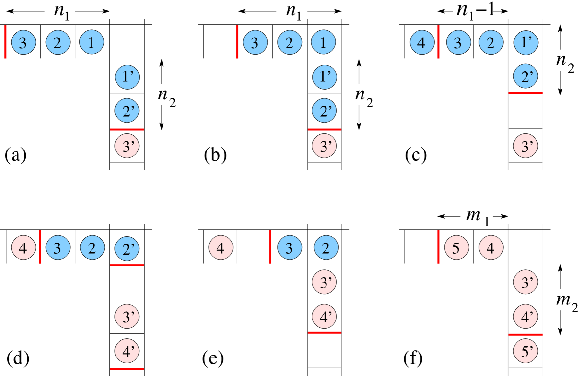
Figure 2: Sequence of snapshots illustrating the pairing effect of platoons at the intersection site. In this example $n_{1}=3$ and $n_{2}=m_{1}=m_{2}=2$. See text.

Figure 2a shows a particle configuration near the exit at some integer instant of time $t=s$ at which the intersection site is empty. A heavy (red) bar (below or to the left of a particle) marks an end-of-platoon. In each lane there is a platoon (dark colored particles) waiting to enter the empty intersection site; the platoons have lengths $n_{1}$ and $n_{2}$ and are headed by the particles marked $1$ and $1^{\prime}$. At the next time step, $t=s+1$, the platoon head with the lower phase will hop onto the intersection site, its whole platoon will advance by one lattice distance, and it will block the other waiting particle. Let us suppose, as shown in figure 2b, that it is the horizontally moving platoon that advances. During each of the next time steps, the lane 1 particle (marked 1), as long as it occupies the exit site, will exit with probability $\beta_{1}$, so it will exit only after on average $\beta_{1}^{-1}$ time steps. During the same time step in which it exits, out of the two particles (marked $2$ and $1^{\prime}$) that are waiting to hop onto the exit site, again the one with the lower phase will effectively hop, pull along its whole platoon, and block the other one. Let us suppose that it is the lane 2 particle (marked 1^′) that advances. This takes us to the configuration of figure 2c. It is equivalent to the one of 2b, except for an interchange of the roles of lanes 1 and 2, accompanied by the replacements $n_{1}\mapsto n_{2}$ and $n_{2}\mapsto n_{1}-1$. The procedure taking us form 2b to 2c will now repeat itself mutatis mutandis  and each time either $n_{1}$ or $n_{2}$ will decrease by one unit. Lane 1 and lane 2 particles have average exit times $\beta_{1}^{-1}$ and $\beta_{2}^{-1}$, respectively. At some point the last particle of one of the two platoons is on the intersection site. Let us suppose this is a lane 2 particle, as in 2d where it is marked $2^{\prime}$. During the same the time step in which $2^{\prime}$ leaves the intersection site, that site will be occupied by the particle waiting in the other lane (marked $2$), which has a higher phase. This will result in the situation of figure 2e. The next lane 2 particle (marked $3^{\prime}$) belongs to the next platoon; if it has already arrived at the waiting site (which may or may not be the case), it will be blocked in that time step. It will similarly be blocked in all following time steps, until the last remaining particle (marked $3$) of the lane 1 platoon leaves the intersection site. The situation that then results is depicted in figure 2f. It is identical to that of figure 2a, except that now the next two platoons, of lengths $m_{1}$ and $m_{2}$ and headed by particles $4$ and $3^{\prime}$, are waiting to enter the intersection site. This is the pairing effect.

We remark parenthetically that this pairing argument is easily extended to an arbitrary number $p$ of lanes intersecting at a single site, when they are all in the jammed phase. We will not, however, attempt to consider here such more general geometries.

We will now exploit this effect to find an expression for the current in the JJ phase. In order to arrive at the situation of figure 2f starting from the one of figure 2a there is first the time step in which the exit site gets occupied. Next, there are $n_{1}$ lane 1 particles and $n_{2}$ lane 2 particles that leave the intersection site subject to the exit probabilities $\beta_{1}$ and $\beta_{2}$, respectively. The total time $t_{n_{1}n_{2}}$ needed for this process and averaged over all exit histories therefore is $t_{n_{1}n_{2}}=n_{1}\beta_{1}^{-1}+n_{2}\beta_{2}^{-1}+1$. Let $\nu_{1}\equiv\nu(\alpha_{1})$ and $\nu_{2}\equiv\nu(\alpha_{2})$ be the average platoon lengths in the two lanes. Then the mean exit time $t_{\rm exit}$ of an arbitrary pair of platoons to exit is the average of $t_{n_{1}n_{2}}$ over all platoon lengths. This yields

$$t_{\rm exit}=\frac{\nu_{1}}{\beta_{1}}+\frac{\nu_{2}}{\beta_{2}}+1.$$ (4.2)

Hence in the JJ phase the outgoing currents $J^{\rm JJ}_{1}$ and $J^{\rm JJ}_{2}$ of the two lanes are given by

$$J^{\rm JJ}_{\sigma}=\frac{\nu_{\sigma}}{\frac{\nu_{1}}{\beta_{1}}+\frac{\nu_{2}}{\beta_{2}}+1},\qquad\sigma=1,2.$$ (4.3)

This expression is a nontrivial generalization of the single lane formula (3.2). Both currents (4.3) depend on all four parameters $\alpha_{1}$, $\alpha_{2}$, $\beta_{1}$, $\beta_{2}$. The ratios $\nu_{\sigma}/\beta_{\sigma}$, which will reappear frequently below, show the scaling with $\beta_{\sigma}$ of the time that the intersection site is occupied by lane $\sigma$ particles.

All elements are in place now for us to go on and find the phase boundaries in the domain $0\leq\alpha_{1},\alpha_{2}\leq 1$.

4.3 Boundaries of the JJ and FJ/JF phases

Let us suppose the system is in the JJ phase. The condition for the system to be able to sustain these queues is that in both lanes the out-current $J^{\rm JJ}_{\sigma}$ be smaller than the corresponding free flow entrance driven current $J^{\rm F}(\alpha_{\sigma})$. That is, for the JJ phase to be stable we should satisfy the two inequalities

$$J^{\rm F}(\alpha_{\sigma})\geq J^{\rm JJ}_{\sigma}\,,\qquad\sigma=1,2,$$ (4.4)

or, upon substituting (4.1) and (4.3) in (4.4),

$$\frac{a_{\sigma}}{1+a_{\sigma}}\geq\frac{\nu_{\sigma}}{\frac{\nu_{1}}{\beta_{1}}+\frac{\nu_{2}}{\beta_{2}}+1}\,,\qquad\sigma=1,2.$$ (4.5)

On the borderline of the JJ phase equation (4.5) should hold as an equality for either $\sigma=1$ or $\sigma=2$. To rewrite this equality we invert both of its members and use (2.4). It then follows that

$$\frac{\nu_{\sigma}}{\alpha_{\sigma}}=\frac{\nu_{1}}{\beta_{1}}+\frac{\nu_{2}}{\beta_{2}}\,,\qquad\sigma=1,2,$$ (4.6)

or, equivalently,

$$\nu_{1}\left(\frac{1}{\alpha_{1}}-\frac{1}{\beta_{1}}\right) = \frac{\nu_{2}}{\beta_{2}}\,,$$ (4.7a)

$$\nu_{2}\left(\frac{1}{\alpha_{2}}-\frac{1}{\beta_{2}}\right) = \frac{\nu_{1}}{\beta_{1}}\,.$$ (4.7b)

Equations (4.7) represent two intersecting curves in the $\alpha_{1}\alpha_{2}$ plane. Although they depend on the parameters $\beta_{1}$ and $\beta_{2}$, their point of intersection always lies on the diagonal $\alpha_{1}=\alpha_{2}$. To see this, note that $\nu_{\sigma}=\nu(\alpha_{\sigma})$ is a function only of $\alpha_{\sigma}$ and hence $\alpha_{1}=\alpha_{2}=\alpha_{\rm c}$ implies that $\nu_{1}=\nu_{2}=\nu_{\rm c}$. Using this in (4.7) we see that $\nu_{\rm c}$ divides out and that both equations are satisfied by

$$\alpha_{\rm c}=\frac{\beta_{1}\beta_{2}}{\beta_{1}+\beta_{2}}\,.$$ (4.8)

Hence equation (4.7a) gives the JJ/FJ boundary in the triangle above the diagonal $\alpha_{1}=\alpha_{2}$ and (4.7b) gives the JJ/JF boundary in the triangle below this diagonal. For the special case $\beta_{1}=\beta_{2}=1$ these phase boundaries are shown in figure 3, which is symmetric with respect to the diagonal. An example of the general case with $\beta_{1}\neq\beta_{2}$ is shown in figure 4, where this symmetry has been lost.

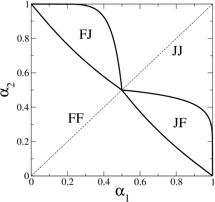
Figure 3: Phase diagram in the $\alpha_{1}\alpha_{2}$ plane for $\beta_{1}=\beta_{2}=1$. The heavy solid lines are phase boundaries. Dashed line: the diagonal. The symbols F (free) and J (jammed) refer to lanes 1 and 2 in the order given. The four-phase point is at $(\alpha_{1},\alpha_{2})=(\tfrac{1}{2},\tfrac{1}{2})$.

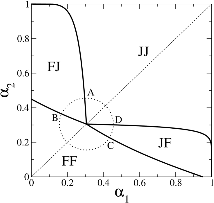
Figure 4: Phase diagram in the $\alpha_{1}\alpha_{2}$ plane for $\beta_{1}=0.95$ and $\beta_{2}=0.45$. All symbols are as in figure 3. The four-phase point is on the diagonal at $(\alpha_{\rm c},\alpha_{\rm c})$ with $\alpha_{\rm c}$ given by (4.8). As shown in section 4.5.2, the boundary curves of the FF phase intersect the $\alpha_{1}$ and $\alpha_{2}$ axes in $\alpha_{1}=\beta_{1}$ and $\alpha_{2}=\beta_{2}$, respectively. Dotted circle: path along which the simulation results of figures 6 and 7 were obtained.

4.4 Boundaries of the FF and FJ/JF phases

We wish to find now the borderline between the FJ and JF phases, on the one hand, and the FF phase on the other hand. To be definite, let us suppose the system is in the FJ phase so that we know that the current in lane 1 is given by its free flow expression

$$J^{\rm FJ}_{1}=J^{\rm F}(\alpha_{1}).$$ (4.9)

The current $J^{\rm FJ}_{2}$ in lane 2 is, however, unknown. In order to calculate $J^{\rm FJ}_{2}$ we cannot invoke now the pairing mechanism, since it requires both  lanes to be jammed. Instead, let us suppose that for every platoon that exits the jammed lane 2, and that is known to contain on average $\nu_{2}$ walkers, there are on average $\mu_{1}$ walkers that exit lane 1. Here $\mu_{1}$ is unknown but necessarily satisfies

$$\mu_{1}\leq\nu_{1}\,.$$ (4.10)

Then we have for the exiting currents in the FJ phase the two asymmetric expressions

$$J^{\rm FJ}_{1} = \frac{\mu_{1}}{\frac{\mu_{1}}{\beta_{1}}+\frac{\nu_{2}}{\beta_{2}}+1}\,,$$ (4.11a)

$$J^{\rm FJ}_{2} = \frac{\nu_{2}}{\frac{\mu_{1}}{\beta_{1}}+\frac{\nu_{2}}{\beta_{2}}+1}\,.$$ (4.11b)

Upon combining (4.9) with (4.11a) and using (3.1) we may solve for $\mu_{1}$ and find

$$\mu_{1}=\frac{\left(\frac{\nu_{2}}{\beta_{2}}+1\right)a_{1}}{1+\left(1-\frac{1}{\beta_{1}}\right)a_{1}}\,.$$ (4.12)

The condition for the sustainability of the jammed phase in lane 2 is

$$J^{\rm F}(\alpha_{2})\geq J^{\rm FJ}_{2}\,.$$ (4.13)

The phase transition line is obtained when (4.13) holds as an equality, which, with the substitutions of (4.11b) and (3.1), happens for

$$\frac{a_{2}}{1+a_{2}} = \frac{\nu_{2}}{\frac{\mu_{1}}{\beta_{1}}+\frac{\nu_{2}}{\beta_{2}}+1}$$ (4.14)

$$= \nu_{2}\,\frac{a_{1}}{1+a_{1}}\,\frac{1+\left(1-\frac{1}{\beta_{1}}\right)a_{1}}{\left(\frac{\nu_{2}}{\beta_{2}}+1\right)a_{1}}$$

$$= \frac{\nu_{2}\beta_{2}}{\nu_{2}+\beta_{2}}\,\frac{1+\left(1-\frac{1}{\beta_{1}}\right)a_{1}}{1+a_{1}}\,,$$

where to pass from the first to the second line we first noticed that by (4.11a) and (4.9) the denominator on the RHS is equal to $\mu_{1}/J^{\rm FJ}_{1}=\mu_{1}/J^{\rm F}(\alpha_{1})=\mu_{1}(1+a_{1})/a_{1}$ and then substituted for $\mu_{1}$ expression (4.12). We may solve (4.14) for $a_{1}$ and find

$$a_{1}=\frac{\beta_{1}(1-R_{2})}{1-\beta_{1}(1-R_{2})}\,,$$ (4.15)

where we introduced the abbreviation $R_{2}\equiv R(\alpha_{2},\beta_{2})$ with

$$R(\alpha,\beta)=\frac{a}{1+a}\,\frac{\nu+\beta}{\nu\beta}\,.$$ (4.16)

We will continue to consider $\beta_{1}$ and $\beta_{2}$ as fixed parameters. When in (4.15) we use (4.16) for $R_{2}$, (2.4) for $\nu_{2}$, and (2.2) for $\alpha_{2}$, it becomes an explicit solution for $a_{1}$ in terms of $a_{2}$, or equivalently, for $\alpha_{1}$ in terms of $\alpha_{2}$ . Hence (4.15) constitutes our final result for the FF/FJ boundary. A permutation of indices gives the FF/JF boundary. These phase boundaries are again shown in figures 3 and 4 for the symmetric case with $\beta_{1}=\beta_{2}=1$ and for a typical asymmetric case, respectively.

4.5 Limiting cases

We consider in this section the limit behavior of the phase boundaries as they approach the borders of the domain $0\leq\alpha_{1},\alpha_{2}\leq 1$.

4.5.1 Boundaries of the JJ phase

One obtains from (4.7a) the behavior of the JJ/FJ boundary in the limit of small $\alpha_{1}$ by noticing that $\lim_{\alpha_{1}\to 0}\nu_{1}=2$ and that therefore in that limit the LHS of (4.7a) diverges, which forces $\nu_{2}$ on the RHS also to diverge. Using next that for $\alpha_{2}\to 1$ one has $\nu_{2}\simeq-\log(1-\alpha_{2})$ one finds

$$\alpha_{2}\simeq 1-{\rm e}^{-2\beta_{2}/\alpha_{1}},\qquad\alpha_{1}\to 0.$$ (4.17)

A permutation of indices gives the asymptotic behavior of the JJ/JF boundary in the limit $\alpha_{2}\to 0$. The exponentials of the inverse functions $1/\alpha_{1}$ and $1/\alpha_{2}$ explain the extremely rapid alignment of these curves along the edges of the figure.

4.5.2 Boundaries of the FF phase

We wish to find the point of intersection of the FF/JF (FF/FJ) boundary with the horizontal (vertical) axis. It is located at $\alpha_{1}=\beta_{1}$ (at $\alpha_{2}=\beta_{2}$). To show this, we ask what the limiting value of $\alpha_{2}$ is when $\alpha_{1}\to 0$. It is useful to notice that the quantity $R_{2}$ that occurs in (4.15) may be expressed as a ratio of two single lane currents,

$$R_{2}=\frac{J^{\rm free}(\alpha_{2})}{J^{\rm jam}(\alpha_{2},\beta_{2})}\,.$$ (4.18)

The ‘physical’ argument goes as follows. For $\alpha_{1}=0$ lane 1 is unoccupied and the intersecting lane problem reduces to that of the single open-ended lane with boundary conditions $(\alpha_{2},\beta_{2})$, whose critical point is known [11] to occur at $\alpha_{2}=\beta_{2}$. Mathematically, $\alpha_{1}=0$ implies $a_{1}=0$; when this is substituted for the LHS of (4.15) we find $R_{2}=1$, after which (4.16) yields $J^{\rm free}(\alpha_{2})=J^{\rm jam}(\alpha_{2},\beta_{2})$. When this equality is worked out we obtain the same result $\alpha_{2}=\beta_{2}$. Finding the limit behavior for $\alpha_{2}\to 0$ amounts to a permutation of indices.

The straight line (not drawn in figures 3 and 4) that connects these two points of intersection has the equation

$$\frac{\alpha_{1}}{\beta_{1}}+\frac{\alpha_{2}}{\beta_{2}}=1$$ (4.19)

and also passes through the critical point $(\alpha_{\rm c},\alpha_{\rm c})$. In both figures, 3 and 4, the boundary delimiting the FF phase is slightly curved and falls just below this straight line.

5 Particle density

The determination of the phase diagram was based exclusively on the analysis of the particle currents in the different phases. From the preceding construction it follows that the currents are continuous at the phase transition lines. This differentiates them from the particle densities, which are the quantities of interest in this section. We will denote a particle density generically by the symbol $\rho$, to which we attach indices according to the same convention as used for $J$. In all phases we have the relation $J=v\rho$, where $\rho$ is the particle density and $v$ the average particle velocity. Since in the free flow phase all particles have velocity $v=1$, we have $\rho^{\rm F}=J^{\rm F}$ and therefore

$$\rho^{\rm FF}_{\sigma}=\frac{a_{\sigma}}{1+a_{\sigma}}\,,\qquad\sigma=1,2,$$ (5.1)

$$\rho^{\rm FJ}_{1}=\frac{a_{1}}{1+a_{1}}\,,\qquad\rho^{\rm JF}_{2}=\frac{a_{2}}{1+a_{2}}\,.$$ (5.2)

In the jammed phase we have generically the relation $J=\nu(1-\rho)$, where $\nu$ is as before the average platoon length. This gives the three relations

$$J^{\rm JJ}_{\sigma}=\nu_{\sigma}(1-\rho^{\rm JJ}_{\sigma}),\qquad\sigma=1,2,$$ (5.3)

$$J^{\rm FJ}_{2}=\nu_{2}(1-\rho^{\rm FJ}_{2}),\qquad J^{\rm JF}_{1}=\nu_{1}(1-\rho^{\rm JF}_{1}).$$ (5.4)

Solving these for the densities using the expressions found in section 4 for the currents we get

$$\rho^{\rm JJ}_{\sigma}=\frac{\frac{\nu_{1}}{\beta_{1}}+\frac{\nu_{2}}{\beta_{2}}}{\frac{\nu_{1}}{\beta_{1}}+\frac{\nu_{2}}{\beta_{2}}+1}\,,\qquad\sigma=1,2,$$ (5.5)

$$\rho^{\rm FJ}_{2}=\frac{\frac{\mu_{1}}{\beta_{1}}+\frac{\nu_{2}}{\beta_{2}}}{\frac{\mu_{1}}{\beta_{1}}+\frac{\nu_{2}}{\beta_{2}}+1}\,,\qquad\rho^{\rm JF}_{1}=\frac{\frac{\nu_{1}}{\beta_{1}}+\frac{\mu_{2}}{\beta_{2}}}{\frac{\nu_{1}}{\beta_{1}}+\frac{\mu_{2}}{\beta_{2}}+1}\,.$$ (5.6)

Remarkably, equation (5.5) shows that in the JJ phase the particle densities in the two lanes are equal irrespective of the values of $\alpha_{1},\alpha_{2},\beta_{1},\beta_{2}$.

Equations (5.1), (5.2), (5.5), and (5.6)constitute our analytic results for the particle densities in the four different phases.

6 Simulations

In order to test the theory of the preceding sections we determined the phase of the system for fixed $\beta_{1}=\beta_{2}=0.6$ on a grid of points in the $\alpha_{1}\alpha_{2}$ plane. The grid was refined in a square region around the four-phase point, which according to equation (4.8) occurs at $(\alpha_{1},\alpha_{2})=(0.3,0.3)$. To determine the phase for a specific pair $(\alpha_{1},\alpha_{2})$, simulations were performed on intersecting lattices of lengths $L_{1}=L_{2}\equiv L=75$. In a finite system the entrance and exit boundary conditions try to impose different phases, which as a consequence will be separated by a domain wall [11, 12, 13, 14]. Away from the critical point the fluctuating domain wall position will be localized within some finite distance from one of the lane ends; upon approach of criticality this localization length increases until it attains the lane length $L$. In our simulations the domain wall position was determined in each lane as described in [11]. We then averaged it over 5 000 000 time steps after having first discarded a transient of 5 000 time steps in order to make sure that the system was stationary. The lane was classified F or J if its mean position was closer to the exit or closer to the entrance, respectively. The results are represented in figure 5. They are in perfect agreement with the theoretical phase boundaries, within the resolution of the grid.

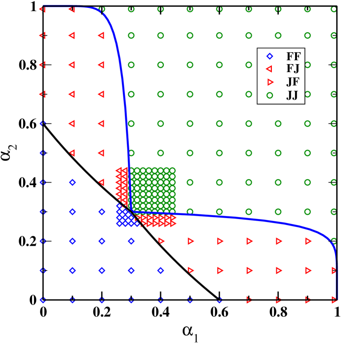
Figure 5: Phase diagram in the $\alpha_{1}\alpha_{2}$ plane for $\beta_{1}=\beta_{2}=0.6$. The nature of the phase was determined (see text) on a grid of points with a denser covering near the four-phase point $(\alpha_{1},\alpha_{2})=(0.3,0.3)$. The phase boundaries are those given by theory.

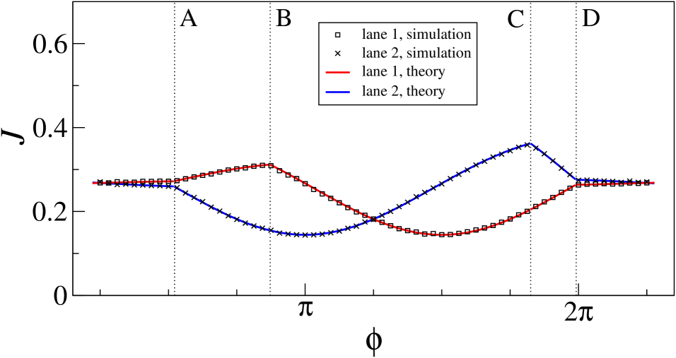
Figure 6: The current, denoted by the generic symbol $J$, as a function of the angle $\phi$ in lanes 1 and 2.

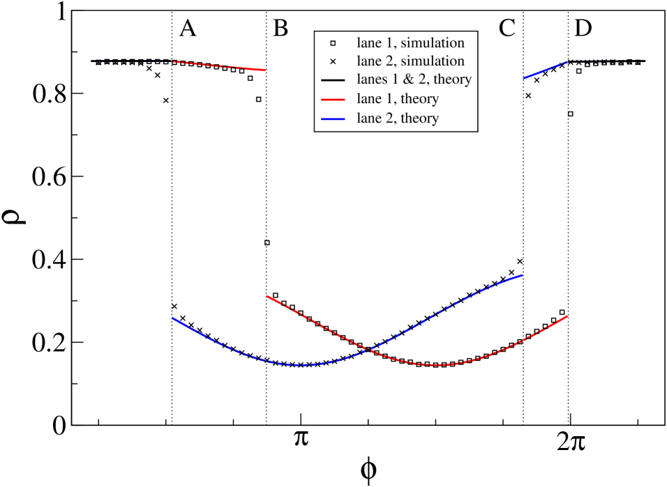
Figure 7: The density, denoted by the generic symbol $\rho$, as a function of the angle $\phi$ in lanes 1 and 2. The black part of the theoretical curves is common to both lanes. Comparison to figure 6 shows that for a lane in the free flow phase we have $J=\rho$.

A more detailed simulation was carried out for the asymmetric case of figure 4. In the $\alpha_{1}\alpha_{2}$ domain we considered the circular path of radius $0.15$ and centered in $(\alpha_{\rm c},\alpha_{\rm c})$, represented in figure 4. In each one of $64$ equidistant points along this circle we determined the stationary state densities $\rho_{1}$ and $\rho_{2}$ as well as the currents $J_{1}$ and $J_{2}$ in the two lanes, for lane length $L=600$. Each data point was obtained by first discarding a transient period of $10\,000$ time steps and then averaging over $100\,000$ time steps. The results, together with the theoretical predictions, are shown in figures 6 and 7, where $\phi$ is the angle between the radius vector on the circle and the positive $\alpha_{1}$ axis. Dotted vertical lines indicate the positions of the phase boundaries, labeled by the same lettering $A,B,C,D$ as in figure 4. The error bars of the data points are smaller than the symbols. The current data of figure 6 fall perfectly on the theoretical curve throughout the whole range of measurements. The density data of figure 7 show a clear deviation from the theoretical prediction at those phase boundaries where the latter is discontinuous. Indeed, the prediction is for lane length $L=\infty$ and these deviations appear to be finite size effects. We have verified that indeed this effect decreases when $L$ goes up. Their physical origin is the same as was found for a single lane [11]: they result from the formation of a fluctuating jammed boundary layer near the exit (when the lane is in its free flow phase), or of a fluctuating free flow boundary layer near the entrance (when the system is in its jammed phase).

7 Conclusion

We have studied pedestrian traffic on two semi-infinite one-dimensional lattices, or lanes, that intersect in a common end point. The pedestrians are modeled as the particles of a TASEP, that is, as hard core particles capable of moving only in a single direction, in the present case toward the exit. When leaving the intersection site, a particle exits the system. The particle positions were updated with ‘frozen shuffle’ dynamics, described in section 2.1 and argued to be a natural choice for pedestrian motion. The updating is easy to implement in a Monte Carlo simulation an also lends itself particularly well to analytical study.

Each of the lanes (labeled by $\sigma=1,2$) is characterized by a parameter $\alpha_{\sigma}$ governing the entrance of the particles at $-\infty$, and another one,$\beta_{\sigma}$, governing their exit from the intersection site. For arbitrary fixed $\beta_{1}$ and $\beta_{2}$ we have determined analytically the phase boundaries in the $\alpha_{1}\alpha_{2}$ plane. It appears that each lane may be in either a free flow (F) or a jammed (J) phase, which results in a partition of the phase diagram in the $\alpha_{1}\alpha_{2}$ plane into four regions, JJ, FJ, JF, and FF. Explicit expressions have been found for the phase boundaries between these regions. An essential element in our analysis is the pairing effect  that we have shown to occur when both lanes are in the jammed phase: in that case each platoon exiting from one lane is accompanied by a platoon exiting from the other lane. Once the pairing effect is established, the analytical expressions for the macroscopic quantities of greatest interest, the currents and the particle densities, become accessible via reasonably simple mathematics. We have determined them analytically for each region of the phase diagram. All our analytical findings have been corroborated by Monte Carlo simulations presented in section 6.

This work is to be seen as a first step towards the study of the intersection of larger corridors, in which case the possibility of lateral hops may also have to be included. We will leave the study of such more complicated geometries and hopping rules to future work.

References

- [1] A. Schadschneider, A. Kirchner, and K. Nishinari. From ant trails to pedestrian dynamics. Applied Bionics and Biomechanics, 1:11–19, 2003.
- [2] C. Burstedde, K. Klauck, A. Schadschneider, and J. Zittartz. Simulation of pedestrian dynamics using a 2-dimensional cellular automaton. Physica A, 295:507–525, 2001.
- [3] N. Rajewsky, L. Santen, A. Schadschneider, and M. Schreckenberg. The asymmetric exclusion process: Comparison of update procedures. J. Stat. Phys., 92:151, 1998.
- [4] M. Wölki, A. Schadschneider, and M. Schreckenberg. Asymmetric exclusion processes with shuffled dynamics. J. Phys. A-Math. Gen., 39:33–44, 2006.
- [5] M. Wölki, A. Schadschneider, and M. Schreckenberg. Asymmetric exclusion processes with non-factorizing steady states. In A. Schadschneider, T. Poschel, R. Kuhne, M. Schreckenberg, and D.E. Wolf, editors, Traffic and Granular Flow ’ 05, pages 473–479, 2007.
- [6] D.A. Smith and R.E. Wilson. Dynamical pair approximation for cellular automata with shuffle update. J. Phys. A: Math. Theor., 40(11):2651–2664, 2007.
- [7] H. Klüpfel. The simulation of crowds at very large events. In A. Schadschneider, T. Poschel, R. Kuhne, M. Schreckenberg, and D.E. Wolf, editors, Traffic and Granular Flow ’05, pages 341–346, 2007.
- [8] A. Kirchner, K. Nishinari, and A. Schadschneider. Friction effects and clogging in a cellular automaton model for pedestrian dynamics. Phys. Rev. E, 67:056122, 2003.
- [9] A. Kirchner, H. Klüpfel, K. Nishinari, A. Schadschneider, and M. Schreckenberg. Simulation of competitive egress behaviour: comparison with aircraft evacuation data. Physica A, 324:689–697, 2003.
- [10] C. Appert-Rolland, J. Cividini, and H. Hilhorst. Frozen shuffle update for an asymmetric exclusion process on a ring. J. Stat. Mech., P07009, 2011.
- [11] C. Appert-Rolland, J. Cividini, and H. Hilhorst. Frozen shuffle update for an asymmetric exclusion process with open boundary conditions. Preprint arXiv:1107.3727, submitted to J. Stat. Mech..
- [12] A.B. Kolomeisky, G.M. Schütz, E.B. Kolomeisky, and J.P. Straley. Phase diagram of one-dimensional driven lattice gases with open boundaries. J. Phys. A: Math. Gen., 31:6911, 1998.
- [13] C. Pigorsch and G.M. Schütz. Shocks in the asymmetric simple exclusion process in a discrete-time update. J. Phys. A: Math. Gen., 33:7919–7933, 2000.
- [14] L. Santen and C. Appert. The asymmetric exclusion process revisited: Fluctuations and dynamics in the domain wall picture. J. Stat. Phys., 106:187–199, 2002.