Hubble’s law and faster than light expansion speeds

Abstract

Naively applying Hubble’s law to a sufficiently distant object gives a receding velocity larger than the speed of light. By discussing a very similar situation in special relativity, we argue that Hubble’s law is meaningful only for nearby objects with non-relativistic receding speeds. To support this claim, we note that in a curved spacetime manifold it is not possible to directly compare tangent vectors at different points, and thus there is no natural definition of relative velocity between two spatially separated objects in cosmology. We clarify the geometrical meaning of the Hubble’s receding speed $v$ by showing that in a Friedmann-Robertson-Walker spacetime if the four-velocity vector of a comoving object is parallel-transported along the straight line in flat comoving coordinates to the position of a second comoving object, then $v/c$ actually becomes the rapidity of the local Lorentz transformation, which maps the fixed four-velocity vector to the transported one.

Hubble’s observations, which showed that the distant galaxies recede with speeds proportional to their distances, marked the beginning of a new era for cosmology hub . Hubble’s results not only changed the widely accepted steady state universe idea, but also provide evidence for the general theory of relativity, which treats spacetime as a dynamical object. Indeed, before Hubble published his observations Friedmann had showed that the Einstein’s equations imply an expanding universe fr . Therefore, in courses about cosmology or general relativity one should certainly discuss Hubble’s law and its consequences.

It is very easy to derive Hubble’s law in the context of a (flat) Friedmann-Robertson-Walker cosmology, which has the line element

$$ds^{2}=-c^{2}dt^{2}+a(t)^{2}\left(dx^{2}+dy^{2}+dz^{2}\right).$$ (1)

The scale factor of the universe $a(t)$ can be thought to define physical lengths so that multiplying the coordinate distance between two points in the space by $a(t)$ gives the physical distance between these points at time $t$. Objects which have constant spatial coordinates $(x,y,z)$ are said to be comoving. The coordinate (or comoving) distance $D_{c}$ between two comoving objects with coordinates $(x_{1},y_{1},z_{1})$ and $(x_{2},y_{2},z_{2})$ is given by $D_{c}=\sqrt{(x_{1}-x_{2})^{2}+(y_{1}-y_{2})^{2}+(z_{1}-z_{2})^{2}}$. The comoving distance $D_{c}$ does not change with time since comoving objects are not moving in space and have fixed positions. However, the physical spatial distance $D$ becomes $D=a(t)D_{c}$. Differentiating $D$ with respect to time $t$ gives the Hubble’s law

$$v=HD,$$ (2)

where the time derivative of the distance is interpreted as the speed, $v=\dot{D}$, and the Hubble parameter is defined as

$$H=\frac{\dot{a}}{a},$$ (3)

where the dot denotes the time derivative.

Despite the simplicity of its derivation, Hubble’s law raises an immediate concern for students: what about the very distant objects whose receding speeds exceed the speed of light? In other words, what happens to the relativistic assumption that nothing can move faster than light? The usual answer to such questions is that the receding speed does not correspond to a physical propagation because the two objects considered in the above derivation are not moving at all. Thus there is no problem for $v$ in (2) to be larger than the speed of light.

Although this explanation of Hubble’s law is certainly correct, one may encounter deeper questions. If the receding velocity due to the expansion of the universe does not quantify a real propagation, what does it physically correspond? Isn’t it the case that to determine the Hubble’s constant $H$, astronomers try to measure the receding velocities of galaxies? How can the measured velocity of an object can be different than the physical propagation velocity of that object with respect to the observer, and if not, how can the propagation velocity be larger than $c$?

There are many misleading statements in the literature about the superluminal receding velocities. These statements are nicely analyzed in l1 ; l2 . Our aim here is not to examine and criticize these statements but to point out that Hubble’s law can be confusing if it is not carefully analyzed. For example, in mc the velocities of recession greater than that of light is said to contradict one of the basic postulates of relativity. Similarly, in the book sc it is claimed that (2) cannot be exact for large distances giving faster than light receding speeds, although we see that the above derivation is straightforward and valid for any distance. (In the same chapter in sc , the claim is clarified by deriving luminosity distance vs. redshift relation and then showing that it reduces to Hubble’s law for nearby objects.) There are also discussions in the literature about the observability of the galaxies with superluminal receding speeds (see e.g. sol1 ; sol2 ; sol3 ).

One reason for the confusion is that neither the speed $v$ nor the distance $D$ can be directly observed. Instead, astronomers measure redshift and luminosity (or angular diameter) distance, which are indirectly related to $v$ and $D$ (see e.g. ha for Hubble’s law expressed as a redshift-distance relation). Of course in a general relativistic framework there must not arise any issue with the faster than light propagation. In any case, however, the relation (2) needs further clarification, at least for students.

The proper language of general relativity is differential geometry, which must also be used in discussing problems in cosmology. Below, we will analyze Hubble’s law in that context. However, students who are acquainted with special relativity can also solve the issue of superluminal receding velocities easily. Consider the following example in special relativity (see e.g. problem 3.5 in ew ). In an inertial frame $S$ two objects A and B are moving along $x$-direction with respective velocities $-2c/3$ and $+2c/3$ (see figure 1). In that frame, the physical distance $L$ between A and B is a well defined quantity. Actually $L$ exactly plays the role of $D$ in Hubble’s law; namely both refer to physical distances in prescribed frames. But, the derivative of $L$ with respect to the time coordinate of the inertial frame $S$ can be found as $\dot{L}=4c/3$, which is larger than $c$. This result does not lead one to think that one of the basic postulates of relativity is violated, because $\dot{L}$ does not give the relative velocity between A and B. It is just the time derivative of a distance and has no direct physical meaning. Only when the speeds of A and B become much smaller than the speed of light, $\dot{L}$ approximates the relative speed, which is equivalent to non-relativistic velocity addition formula. To find the correct relative velocity, one should use relativistic velocity addition formula or equivalently apply a Lorentz transformation to the rest frame $\tilde{S}$ of, say A. Only then can the derivative of the distance $\tilde{L}$ in the frame $\tilde{S}$ with respect to the time parameter of $\tilde{S}$ be interpreted as the relative speed, which is $12c/13<c$ using the relativistic velocity addition formula (see figure 1).

Figure 1: In an inertial frame $S$ the rate of change of the distance $L$ between the objects A and B is $4c/3$, which is larger than the speed of light. On the other hand, in the rest frame $\tilde{S}$ of A the rate of change of the new distance $\tilde{L}$ with respect to the new time parameter is less than $c$

To have a better understanding of this example, let us parametrize the position four-vectors of A and B in the frame $S$ as $x^{\mu}_{A}=(ct,-2ct/3,0,0)$ and $x^{\mu}_{B}=(ct,+2ct/3,0,0)$, where $t$ is the time parameter of $S$. The physical distance $L$ in the frame $S$ can be given as $L^{2}=\eta_{\mu\nu}(x_{A}^{\mu}-x_{B}^{\mu})(x_{A}^{\nu}-x_{B}^{\nu})$, where the metric is given by $\eta_{\mu\nu}=\textrm{diag}(-1,1,1,1)$. Although $L$ can be recast to an invariant quantity, its derivative with respect to time $t$ cannot. The lesson from special relativity is that the time derivative of the distance between two objects does not necessarily give the relative speed, or to be more precise it does not correspond to a physically meaningful quantity.

The situation with the Hubble’s law $v=HD$ is similar. If $v$ is small, it can be approximately interpreted as the relative velocity between two comoving objects (more on this below). Otherwise, it does not have a direct physical meaning, i.e. it does not give us any physical information. Therefore, there is no need to bother about superluminal receding velocities, which would be similar to worrying about $\dot{L}>c$ in the previous example. This fact must clearly be emphasized in teaching Hubble’s law to avoid confusion.

Before discussing the issue in the language of differential geometry, let us try to clarify a possible concern that might occur about the analogy we have discussed. Although students might be convinced by our example from special relativity that the time derivative of a distance does not necessarily give the velocity, it does correctly give the relative velocity in the rest frame of A as shown in figure 1. Then, how can we make sure that the frame in which the Hubble’s law is expressed is not special? Can this frame, in which the comoving objects do not move, be similar to the rest frame of A?. Unfortunately it is not possible to answer such a question without properly discussing the problem in general relativity. There is in principle no difference between the frames $S$ and $\tilde{S}$ in special relativity, since both of them are inertial. Similarly, all frames in general relativity are on an equal footing. In our example, the definition of relative velocity turns out to be equivalent to the time derivative of the distance between two objects in a frame in which one object is stationary.

We now discuss how Hubble’s law should be understood in the general relativity. We first emphasize the following well known but occasionally forgotten fact from differential geometry: in a manifold there is no natural way of comparing tangent vectors at different points unless a connection is introduced as an extra structure (see e.g. w ). One cannot move vectors around, as is usually done in the flat Euclidean space, where there exists a well defined global notion of what it means to be parallel. Only vectors defined in the same tangent space about a point can be compared, added or subtracted. Once a connection (or a covariant derivative associated with a metric) is introduced, parallel-transportation of a vector along a given path can be defined. In that case a vector can be carried out by parallel-transportation along a specified curve from its original position to the position of another vector, and then these two vectors placed in the same position can be compared with each other. However, parallel-transportation is path dependent and thus this comparison is not unique.

These comments are valid for cosmology, despite the fact that at a fixed time the space is the usual euclidean 3-space in (1). Therefore, there is no natural way of comparing four-velocity vectors of two spatially separated objects. Relative velocity can only be defined for two objects passing through the same spacetime point. Note that the situation is different in special relativity, where the underlying Minkowski spacetime is flat and there is a global notion of parallel-ness.

Consider two comoving objects A and B in (1), which are located along the $x$-axis with $D_{c}$ being the coordinate distance between them, as shown in figure 2. The four-velocity vectors of A and B are given by $v_{A}^{\mu}=(1,0,0,0)$ and $v_{B}^{\mu}=(1,0,0,0)$, where the indices refer to the coordinate basis in (1) with $x^{\mu}=(t,x,y,z)$ (in the following discussion we use geometrical units such that $c=1$). To compare velocities let us parallel-transport $v_{A}^{\mu}$ along the $x$-axis at a fixed time to the position of the object B. The tangent vector to this curve, which is the $x$-axis, is given by

$$k^{\mu}=(0,1,0,0).$$ (4)

As mentioned, choosing different paths would give different vectors at B, and there is no natural definition of relative velocity. Nevertheless, we will show that using parallel-transportation along the $x$-axis gives a reasonable generalization of the familiar concept of relative velocity.

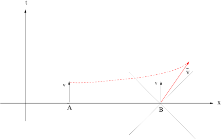
Figure 2: The parallel-transportation of the four-velocity vector of A along the straight line joining A to B. The dashed lines on B represent the light cone. Since parallel-transportation preserves the length of a vector, the transported vector at B is also time-like.

The parallel-transport of a vector $v^{\mu}$ along a curve with tangent $k^{\mu}$ is defined as

$$k^{\mu}\nabla_{\mu}v^{\nu}=0.$$ (5)

This gives a set of coupled first-order differential equation for the components $v^{\mu}$, which are uniquely determined once an initial vector is specified. In our example, the initial vector is $v_{A}^{\mu}$ and one can see that $v^{y}=v^{z}=0$ is the unique solution of (5) with the prescribed initial conditions. For the other two components $v^{t}$ and $v^{x}$, the definition (5) explicitly becomes

$$\partial_{x}v^{t}+\Gamma^{t}{}_{xx}v^{x}=0,$$

$$\partial_{x}v^{x}+\Gamma^{x}{}_{xt}v^{t}=0,$$ (6)

where $(\ref{k})$ has been used. The relevant components of the Christoffel symbol of (1) can be found as

$$\Gamma^{t}{}_{xx}=a\dot{a},\hskip 14.22636pt\Gamma^{x}{}_{xt}=\frac{\dot{a}}{a}.$$ (7)

Defining the orthonormal frame components as

$$v^{\hat{t}}=v^{t},$$

$$v^{\hat{x}}=a\,v^{x},$$

the equation system (6) becomes

$$\partial_{x}v^{\hat{t}}+\dot{a}v^{\hat{x}}=0,$$

$$\partial_{x}v^{\hat{x}}+\dot{a}v^{\hat{t}}=0.$$

These coupled equations can be solved giving

$$\left[\begin{array}[]{c}v^{\hat{t}}\\ v^{\hat{x}}\end{array}\right]=\exp\left(-\left[\begin{array}[]{cc}0&\dot{a}\\ \dot{a}&0\end{array}\right]x\right)\left[\begin{array}[]{c}v^{\hat{t}}_{0}\\ v^{\hat{x}}_{0}\end{array}\right],$$ (14)

where $v^{\hat{t}}_{0}$ and $v^{\hat{x}}_{0}$ are the components of the initial vector. The exponential can be calculated by diagonalization, which gives

$$\left[\begin{array}[]{c}v^{\hat{t}}\\ v^{\hat{x}}\end{array}\right]=\left[\begin{array}[]{cc}\cosh(\dot{a}x)&-\sinh(\dot{a}x)\\ -\sinh(\dot{a}x)&\cosh(\dot{a}x)\end{array}\right]\left[\begin{array}[]{c}v^{\hat{t}}_{0}\\ v^{\hat{x}}_{0}\end{array}\right].$$ (21)

Using $x=D_{c}$, $D=aD_{c}$ and

$$v=HD=\dot{a}D_{c},$$ (22)

one can determine $\tilde{v}^{\mu}$, the transported four-velocity vector of A to the position of B, as

$$\left[\begin{array}[]{c}\tilde{v}^{\hat{t}}\\ \tilde{v}^{\hat{x}}\end{array}\right] = \left[\begin{array}[]{cc}\cosh(v)&-\sinh(v)\\ -\sinh(v)&\cosh(v)\end{array}\right]\left[\begin{array}[]{c}1\\ 0\end{array}\right]$$ (29)

$$= \left[\begin{array}[]{c}\cosh(v)\\ -\sinh(v)\end{array}\right].$$ (32)

Because parallel-transportation preserves the norm, the transported vector $\tilde{v}^{\mu}$ becomes a time-like vector obeying $\tilde{v}^{\mu}\tilde{v}_{\mu}=-1$ (see figure 2).

We have now two vectors $v_{B}^{\mu}$ and $\tilde{v}^{\mu}$ in the same tangent space at the point B. To determine the relative speed between $v_{B}^{\mu}$ and $\tilde{v}^{\mu}$, we note that (29) is equivalent to a Lorentz transformation in the tangent space, which actually maps $v_{B}^{\mu}$ to $\tilde{v}^{\mu}$, where $v$ is the corresponding rapidity parameter related to the Lorentz factor as $\gamma=\cosh(v)$. Therefore, the velocity giving the boost in (29) can be identified as the relative velocity $v_{rel}$. Introducing the factors of $c$ and nothing that $\gamma=1/\sqrt{1-v_{rel}^{2}/c^{2}}$, one finds

$$v_{rel}=c\,\tanh\left(\frac{v}{c}\right).$$ (33)

Thus, we have shown that Hubble’s speed $v$ actually becomes the rapidity of the local Lorentz transformation, which maps the original four-velocity vector of the object B to the parallel-transported four-velocity vector of the object A. In this way one sees that there is no faster than light propagation issue and from (33) the path dependent relative velocity becomes

$$v_{rel}<c$$ (34)

since $\tanh$ function is strictly less than one.

Note that for $v\ll c$ one finds

$$v_{rel}\simeq v.$$ (35)

As expected, Hubble’s receding velocity can be thought to give the relative velocity between two close comoving objects. It is also possible to reinterpret (35) by reversing the logic. Since Hubble’s receding velocity is supposed to give the relative velocity, it is natural to define $v_{rel}$ by parallel-transportation along the straight line joining two comoving objects at a fixed time, at least for nearby objects. For larger distances, one can imagine infinitesimally separated comoving observers placed in between A and B. Nearby observers can measure their relative velocities at a fixed time. From that information, relative velocity between distant objects A and B can be determined by integration, which indeed corresponds to parallel-transportation along the finite line-segment and thus we obtain (33). Consequently, $v_{rel}$ can be seen to generalize the usual concept of relative velocity in a cosmological context.

In summary, we believe that the best way to resolve concerns about superluminal expansion speeds is to emphasize that Hubble’s law does not make sense for large distances. We showed that if the time derivative of the distance between two objects is naively identified as the relative velocity, then faster than light speeds can also be found in special relativity. Therefore, we need to be careful in determining the correct physical meaning of a mathematical quantity in a relativistic theory, which is also the main issue with Hubble’s law. These examples can be used to convince students that there is nothing wrong with a naive superluminal expansion speed since it has nothing to do with relative velocity or as a matter of fact it has no direct physical significance. Moreover, we pinned down the correct differential geometrical meaning of the Hubble’s receding velocity as the rapidity of a local Lorentz transformation. With the derivation of this last result, there must not arise any further issue with faster than light expansion speeds.

References

- (1)
- (2) E. Hubble, A Relation between Distance and Radial Velocity among Extra-Galactic Nebulae, Proc. N.A.S. 15(3), 168–173, (1929).
- (3)
- (4) A. Friedman, Über die Krümmung des Raumes, Z. Phys. 10, 377 -386 (1922). (English translation in: Gen. Rel. Grav. 31, 1991- 2000 (1999).)
- (5)
- (6) T. M. Davis and C. H. Lineweaver, Expanding confusion: common misconceptions of cosmological horizons and the superluminal expansion of the universe, Publ. Astronom. Soc. Aust. 21 (2004) 97, astro-ph/0310808.
- (7)
- (8) T. M. Davis and C. H. Lineweaver, Misconceptions about Big Bang, Scientific American, February 21 (2005) 27.
- (9)
- (10) G.C. Mc Vittie, Distance and large redshifts, Q. Jl R. astr. Soc. 15 (1974) 246.
- (11)
- (12) B.F. Schutz, A First Course in General Relativity, Cambridge University Press, 1985.
- (13)
- (14) H.S. Murdoch, Recession velocities greater than light, Q. Jl R. astr. Soc. 18 (1977) 242.
- (15)
- (16) A.N. Silverman, Resolution of a cosmological paradox using concepts from general relativity theory, Am. J. Phys. 12 (1986) 1092.
- (17)
- (18) W.M. Stuckey, Can galaxies exist within our particle horizon with Hubble recessional velocities greater than , Am. J. Phys. 60 (1992) 142.
- (19)
- (20) E. Harrison, The redshift-distance and velocity-distance laws, The Astrophysical Journal, 403 (1993) 20.
- (21)
- (22) G.F.R. Ellis and R.M. Williams, Flat and curved space-times, Oxford University Press, 2000.
- (23)
- (24) R.M. Wald, General relativity, University Of Chicago Press, 1984.
- (25)