Adaptive Tuning of Feedback Gain in Time-Delayed Feedback Control

Abstract

We demonstrate that time-delayed feedback control can be improved by adaptively tuning the feedback gain. This adaptive controller is applied to the stabilization of an unstable fixed point and an unstable periodic orbit embedded in a chaotic attractor. The adaptation algorithm is constructed using the speed-gradient method of control theory. Our computer simulations show that the adaptation algorithm can find an appropriate value of the feedback gain for single and multiple delays. Furthermore, we show that our method is robust to noise and different initial conditions.

The control of nonlinear systems is a central topic in dynamical system theory, with a diverse range of applications. Adaptive control schemes have emerged as a new type of control method that optimizes the control parameters with respect to an appropriate goal function, thereby minimizing, for instance, the consumed power or the time needed to reach the control goal. In this work we combine time-delayed feedback control, an established method from chaos control, with an adaptive speed-gradient scheme to optimize the control force. We demonstrate how this combined scheme can be utilized to stabilize various target states, e.g., unstable fixed points or periodic orbits, with little or no apriori knowledge about the target state. We also investigate the robustness of the method to noise and perturbations.

I Introduction

Stabilization of unstable and chaotic systems forms an important field of research in nonlinear dynamics. A variety of control schemes have been developed to control periodic orbits as well as steady states OTT90 ; SCH07 . A simple and efficient scheme, introduced by Pyragas PYR92 , is known as time-delay autosynchronization (TDAS). This control method generates a feedback from the difference of the current state of a system to its counterpart some time units $\tau$ in the past. Thus, the control scheme does not rely on a reference system and has only a small number of control parameters, i.e., the feedback gain $K$ and time delay $\tau$. It has been shown that TDAS can stabilize both unstable periodic orbits, e.g., embedded in a strange attractor PYR92 ; BAL05 as well as unstable steady states AHL04 ; ROS04a ; HOE05 . In the first case, TDAS is most efficient and noninvasive if $\tau$ corresponds to an integer multiple of the minimal period of the orbit. In the latter case, the method works best if the time delay is related to an intrinsic characteristic timescale given by the imaginary part of the system’s eigenvalue HOE05 . A generalization of the original Pyragas scheme, suggested by Socolar et al. SOC94 , uses multiple time delays. This extended time-delay autosynchronization (ETDAS) introduces a memory parameter $R$, which serves as a weight of states further in the past. In Ref. DAH07, it is shown that, this method is able to control an unstable fixed points for a larger range of parameters compared to the original TDAS scheme. A variety of analytic results about time-delayed feedback control are known BLE96 ; JUS97 ; JUS98 ; PYR01 , for instance, in the case of long time delays YAN06 , transient behavior HIN11 , unstable spatio-temporal patterns BAB02 , or regarding the odd number limitation NAK97 , which was refuted in Refs. FIE07, ; JUS07, .

In the present paper, we apply the speed-gradient method FRA79 ; FRA98a ; FRA05b ; FRA07 ; GUZ08 to adaptively tune the feedback gain $K$, which is used in both TDAS and ETDAS control methods, and utilize this scheme to stabilize an unstable focus in a generic model, and an unstable periodic orbit embedded in a chaotic attractor. The former model is the generic linearization of a system with an unstable fixed point close to a Hopf bifurcation. The speed-gradient method is a well known adaptive control technique that minimizes a predefined goal function by changing an accessible system parameter appropriately. The adaptation of the feedback gain may be useful, in particular, for systems with slowly changing parameters or when the domain of stability is unknown. There are several other approaches to adaptive control of nonlinear systems in the control literature FRA99a ; AST08a ; KRS95 . Here we have chosen the speed-gradient method because it is simple and robust.

This paper is organized as follows: In Sec. II, we develop the adaptation algorithm using the example of an unstable focus. In Sec. III, we apply the adaptive control scheme to stabilize an unstable periodic orbit embedded in the chaotic attractor of the Rössler system. Finally, we conclude with Sec. IV.

II Stabilization of an unstable fixed point

First, we will consider stabilization of an unstable fixed point by time-delayed feedback. Unlike in previous works (see e.g. HOE05 ; DAH07 and references therein), we do not fix the feedback gain a priori, but tune it adaptively. We consider a general dynamical system given by a nonlinear vector field ${\bf f}$:

$$\dot{\bf X}(t)={\bf f}[{\bf X}(t)]$$ (1)

with ${\bf X}\in\mathbb{R}^{n}$ and an unstable fixed point ${\bf X}^{*}$ solving ${\bf f}({\bf X^{*}})=0$. The stability of this fixed point is obtained by linearizing the vector field around ${\bf X}^{*}$. Without loss of generality, let us assume ${\bf X}^{*}=0$. In the following we will consider the generic case of a two-dimensional unstable focus, i.e., a system close to a Hopf bifurcation, for which the linearized equations can be written in center manifold coordinates $x,y\in\mathbb{R}$ as follows:

$$\dot{x} = \lambda\,x+\omega\,y$$ (2a)

$$\dot{y} = -\omega\,x+\lambda\,y,$$ (2b)

where $\lambda$ and $\omega$ are positive real numbers. $\lambda$ may be viewed as the bifurcation parameter governing the distance from the instability threshold, i.e., a Hopf bifurcation, and $\omega$ is the intrinsic eigenfrequency of the focus. For notational convenience, Eq. (2) can be rewritten as

$$\dot{\bf X}(t)={\bf A}\;{\bf X}(t).$$ (3)

The eigenvalues $\Lambda_{0}$ of the $2\times 2$ matrix ${\bf A}$ are given by $\Lambda_{0}=\lambda\pm i\omega$, so that for $\lambda>0$ and $\omega\neq 0$ the fixed point is an unstable focus. We now apply time-delayed feedback control PYR92 in order to stabilize this fixed point:

$$\dot{x}(t) = \lambda\,x(t)+\omega\,y(t)-K[x(t)-x(t-\tau)]$$ (4a)

$$\dot{y}(t) = -\omega\,x(t)+\lambda\,y(t)-K[y(t)-y(t-\tau)],$$ (4b)

where the feedback gain $K$ and the time delay $\tau$ are real numbers. We assume that the value of $\tau$ is known and appropriately chosen. Mathematically speaking, the goal of the control method is to change the sign of the real part of the eigenvalue, leading to a decay of perturbations from the target fixed point.

Since the control force applied to the $i$th component of the system involves only the same component, this control scheme is called diagonal coupling BEC02 and is suitable for an analytical treatment. Note that the feedback term vanishes if the fixed point is stabilized since $x^{*}(t-\tau)=x^{*}(t)$ and $y^{*}(t-\tau)=y^{*}(t)$ for all $t$, indicating the noninvasiveness of the TDAS method.

To obtain an adaptation algorithm for the feedback gain $K$ according to the standard procedure of the speed-gradient method FRA98a ; FRA05b ; FRA07 ; GUZ08 ; AST08 , let us choose the goal function or cost function as follows:

$$Q({\bf X})=\frac{1}{2}\left\{[x(t)-x(t-\tau)]^{2}+[y(t)-y(t-\tau)]^{2}\right\}.$$ (5)

Successful control yields $Q({\bf X}(t))\rightarrow 0$ as $t\rightarrow\infty$. The speed-gradient algorithm in the differential form is given by $\dot{K}=-\gamma\nabla_{K}\dot{Q}$, where $\gamma>0$ is the adaptation gain and $\nabla_{K}$ denotes $\partial/\partial K$ . Thus, we need to calculate the gradient – with respect to the feedback gain $K$ – of the rate of change of the cost function. For the above cost function Eq. (5) we obtain:

$$\dot{Q} = [x(t)-x(t-\tau)][\dot{x}(t)-\dot{x}(t-\tau)]+[y(t)-y(t-\tau))][\dot{y}(t)-\dot{y}(t-\tau)].$$ (6)

The time derivatives of $x$ and $y$ are given by Eqs.(4). Thus, the speed-gradient method leads to the following equation for the feedback gain:

$$\dot{K}(t) = \gamma\{[x(t)-x(t-\tau)][x(t)-2x(t-\tau)+x(t-2\tau)]+[y(t)-y(t-\tau)][y(t)-2y(t-\tau)+y(t-2\tau)]\}.$$ (7)

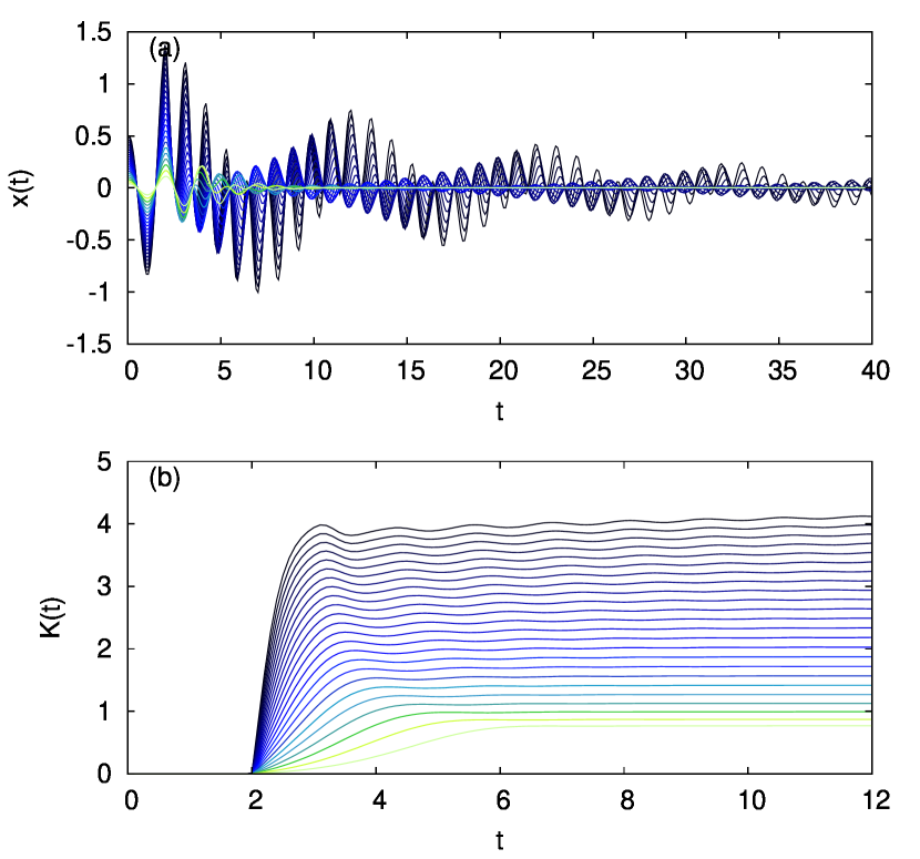
Figure 1: (Color online) Adaptive control of the fixed point: (a) Time series $x(t)$ and (b) feedback gain $K(t)$ for different initial conditions: $x(0)\in[0.02,0.5]$ in steps of 0.02 (from light (green) to dark (blue); in panel (b) from top to bottom), $y(0)=0$. Parameters: $\lambda=0.5$, $\omega=\pi$, $\gamma=1$, $\tau=1$.

Owing to homogeneity the right hand sides of Eqs. (4) and (7), without loss of generality the adaptation gain $\gamma$ can be chosen as 1, because Eqs. (4) and (7) can be rescaled by transformation $x(t)\longrightarrow x(t)/\sqrt{\gamma}$ and $y(t)\longrightarrow y(t)/\sqrt{\gamma}$.

Figure 1 depicts the time series of $x$ and $K$ according to Eqs. (4) and (7) for different initial conditions $x(0)\in[0.02,0.5]$ in steps of 0.02 from light (green) to dark (blue) and $y(0)=0$. In all simulations $x(t)=y(t)=0$ for $t<0$ and $K(t)=0$ for $t\leq 2\tau$. The parameters are chosen as $\lambda=0.5$, $\omega=\pi$, and $\tau=1$. Figure 1(a) shows that the adaptation algorithm works for a large range of initial conditions. Naturally, for initial conditions close to the fixed point the goal is reached faster. If the system starts initially too far from the fixed point ($x(0)>0.85$, $y(0)=0$) the control fails (curves not shown). Note, however, that the basin of attraction can be enlarged by increasing $\gamma$. In fact, due to the scaling, invariance, the maximum value of $|x(0)|$ that still leads to successful control is proportional to $\sqrt{\gamma}$.

In Ref. HOE05, it was shown that in the $(K,\tau)$-plane tongues exist for which the fixed point can be stabilized, i.e., for a given $\tau$ there is a $K$-interval for which the control is successful. As can be seen in Fig. 1(b), the adaptive algorithm converges to some appropriate value of $K$ in this interval depending upon the initial conditions.

Figure 2 demonstrates that the algorithm works for a range of $\tau$, i.e., for any value of $\tau$ within the domain of stability of the TDAS control HOE05 . Black empty circles depict the transient time $t_{c}$ after which the control goal is reached in dependence on the time delay $\tau$. This is the case if the cost function $Q$ becomes sufficiently small. We define the transient time by the bound $\left<Q\right>\equiv\int_{t_{c}-2\tau}^{t_{c}}Q(t^{\prime})dt^{\prime}<2\tau\times 10^{-10}$. The dark (dark purple) shaded regions correspond to the analytically obtained $\tau$-intervals of the Pyragas control HOE05 . Inside these intervals, $t_{c}$ has a finite value confirming that the adaptive control scheme adjusts the feedback gain $K$ to an appropriate value. For a comparison with the transient time of TDAS see Ref. HIN11, where a power law scaling $t_{c}\sim(K-K_{c})^{-1}$ with respect to the fixed feedback gain $K$ has been found (here $K_{c}$ corresponds to the boundaries of stability). The curves corresponding to non-zero memory parameter $R$ (crosses and squares) will be discussed below where the speed-gradient method is applied to the ETDAS scheme.

For a thorough analysis of the stability of the fixed point, we perform a linear stability analysis for the system Eqs. (4), (7). This system has the fixed point $(0,0,K^{*})$ for any $K^{*}=const$. Linearization around the fixed point and the ansatz $\delta x,\delta y,\delta K\propto\exp(\Lambda t)$ yields a transcendental eigenvalue equation

$$0 = \det\left[\begin{array}[]{ccc}\lambda-K(1-e^{-\Lambda\tau})-\Lambda&\omega&0\\ -\omega&\lambda-K(1-e^{-\Lambda\tau})-\Lambda&0\\ 0&0&-\Lambda\end{array}\right]$$ (11)

$$= -\Lambda[\lambda+i\omega-K(1-e^{-\Lambda\tau})-\Lambda][\lambda-i\omega-K(1-e^{-\Lambda\tau})-\Lambda],$$ (12)

which can be solved numerically. This equation is equal to the case of Pyragas control with constant feedback gain considered in Ref. HOE05, except for the factor $\Lambda$. Thus, the adaptively controlled system has an additional eigenvalue at $\Lambda=0$. It results from the translation invariance of the system in the direction of $K$ on the fixed point line $(0,0,K)$. This means that the $K$ values found in the case of the standard Pyragas control lead again to a stabilization of the fixed point. The advantage of an adaptive controller is that an appropriate feedback gain is realized in an automated way, i.e., without prior knowledge of the domain of stability, as long as a stability domain exists for this value of $\tau$.

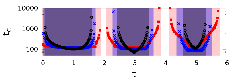
Figure 2: (Color online) Transient time $t_{c}$ after which the control goal is reached in dependence of the delay time $\tau$ for TDAS (black circles) and ETDAS with $R=0.35$ ((blue) crosses), and $R=0.95$ ((red) squares). The dark (dark purple), medium (bright purple), and light (red) shaded regions denote the possible range of $\tau$ for $R=0,0.35$, and $0.95$, respectively. Parameters as in Fig. 1.

An additional advantage of an adaptive control scheme is that it allows one to follow slow changes of the system parameters, which are usually present in experimental situations. To test the ability of our adaptive control scheme to cope with such parameter drifts, we slowly vary $\lambda$ in the following way: $\lambda(t)=0.01+1.8\sin(0.001t)$. The result is illustrated in Fig. 3. In Fig. 3(a) the region of stability of the standard Pyragas control in the ($\lambda,K$) plane (see Ref. HOE05, ) is marked by green (gray) shading. If now $\lambda$ is slowly increased from its initial value 0.01, $K$ follows the change in such a way that whenever the lower boundary of the stability region is crossed and the fixed point becomes unstable, the adaptation algorithm adjusts $K$ such that the stable region is re-entered. This creates a step-like trajectory in the ($\lambda,K$) plane, which is depicted as a red (solid) curve with an arrow. Finally, if $\lambda$ is decreased again, $K$ does not change because it already has attained a value for which the control works in a broad $\lambda$-interval resulting in a horizontal trajectory in the ($\lambda,K$) plane. Fig. 3(b) depicts the corresponding time series of $K(t)$ as a blue (solid) curve, and of the drifting parameter $\lambda(t)$ as a red (dashed) curve, respectively.

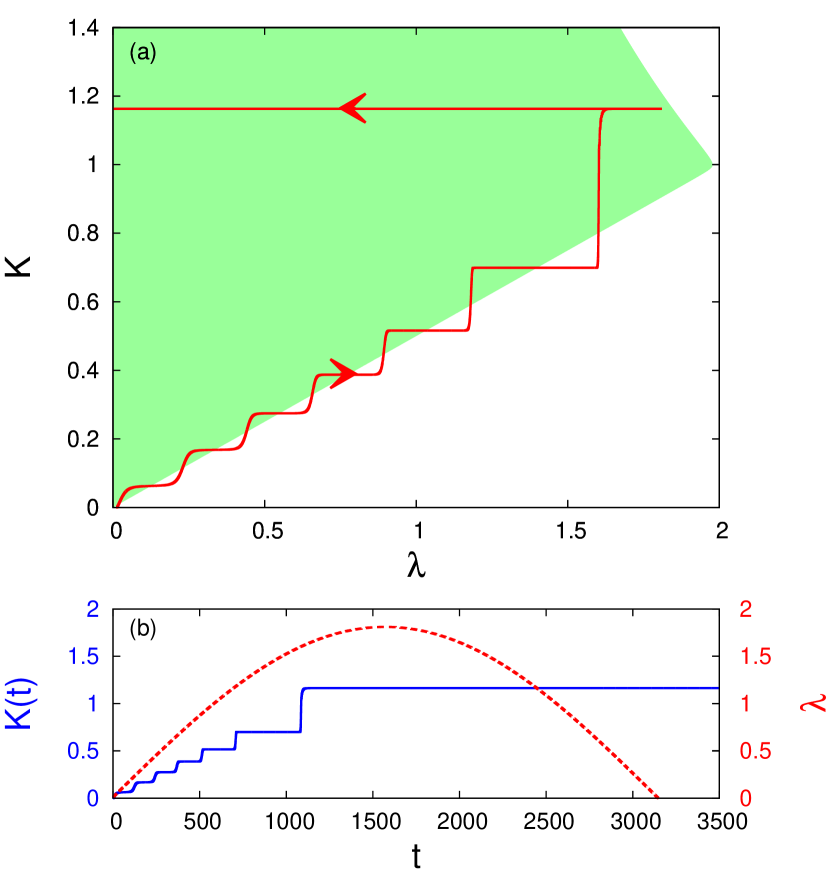
Figure 3: (Color online) Adaptive control of the fixed point for slowly drifting system parameter $\lambda$. (a) Adaptive adjustment of $K$ in the ($\lambda,K$) plane. Green (gray) shaded region: region of stability of the standard Pyragas control. Red (solid) line with arrow: adaptation of feedback gain $K$ if $\lambda$ is slowly changed ($\lambda(t)=0.01+1.8\sin(0.001t)$) (b) Corresponding time series $K(t)$ (blue solid line) and $\lambda(t)$ (dashed red line). Other parameters as in Fig. 1.

To test the robustness of the control algorithm, we add Gaussian white noise $\xi_{i}$ ($i=1,2$) with zero mean and unity variance ($\langle\xi_{i}(t)\rangle=0$, $\langle\xi_{i}(t)\xi_{j}(t-t^{\prime})\rangle=\delta_{ij}\delta(t-t^{\prime})$) to the system variables $x$ and $y$:

$$\dot{x}(t) = \lambda\,x(t)+\omega\,y(t)$$ (13a)

$$-K(t)[x(t)-x(t-\tau)]+D\xi_{1}(t)$$

$$\dot{y}(t) = -\omega\,x(t)+\lambda\,y(t)$$ (13b)

$$-K(t)[y(t)-y(t-\tau)]+D\xi_{2}(t),$$

where $D$ is the strength of the noise.

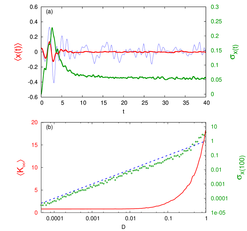
Figure 4: (Color online) Robustness to noise. (a): Thick solid (red) curve: ensemble average $\langle x(t)\rangle$ of 200 realizations; thin (blue) curve: $x(t)$ for one example trial; gray (green) curve: corresponding standard deviation $\sigma_{x(t)}$ of $x(t)$ for a fixed noise intensity $D=0.1$. (b): (Green) crosses: standard deviation $\sigma_{x(100)}$ of $\langle x(t=100)\rangle$; dashed (blue) line: standard deviation of the input noise given by $D$; black (red) curve: asymptotic value $K_{\infty}$ of the feedback gain. Parameters: $\gamma=0.001$, $x(0)=0.05$, $y(0)=0$. Other parameters as in Fig.1.

In Fig. 4(a) the ensemble average over 200 realizations, i.e., $\langle x(t)\rangle=1/200\sum^{200}_{i=1}x_{i}(t)$, for $D=0.1$ (intermediate noise) is depicted as a solid (red) curve. The thin (blue) curve exemplarily depicts one realization. The corresponding standard deviation $\sigma_{x(t)}$ of $x(t)$ is shown as a gray (green) curve. The control is successful in all realizations: For large $t$ the mean $\langle x(t)\rangle$ fluctuates around the fixed point value at zero, due to the finite number of realizations. The standard deviation approaches a value smaller than the standard deviation of the input noise.

This is further elaborated in Fig. 4(b), which depicts the standard deviation $\sigma_{x}$ at $t=100$ versus the noise strength $D$ as (green) crosses. If $D$ becomes too large the standard deviation exceeds the one of the input noise indicated by the dashed (blue) line. This is the case for $D\gtrsim 0.4$. Then the control algorithm will generally fail (time series not shown here): The oscillations of $x(t)$ become larger with increasing $t$. Accordingly, the standard deviation $\sigma_{x(t)}$ increases with $t$ indicating that the dynamics is dominated by noise which forces at least some of the realizations to diverge. The black (red) curve in Fig. 4(b) depicts the asymptotic value $K_{\infty}$ of the feedback gain. For intermediate noise strength, an increased feedback gain $K$ compensates the influence of noise ensuring that the control is still successful. For too large $D$, $K$ increases to a value beyond the domain of stability and stabilization cannot be achieved.

We conclude that the adaptive algorithm is quite robust to noise (the escape rate is vanishingly small for $D\lesssim 0.4$) and only fails for large noise ($D\gtrsim 0.4$). Our method allows for finding the appropriate $K$ for all values of $\tau$ for which the standard Pyragas control stabilizes the fixed point and is able to follow slow drifts in the system parameters.

Note that the method still works if the control term is added only to the $x$-component. Then, using $Q(x)=[x(t)-x(t-\tau)]^{2}/2$ as a goal function leads to qualitatively very similar results. This observation becomes relevant for experimental realizations of the time-delayed feedback control when only certain components of the system under control are accessible for measurements FLU11 .

Next, we consider the ETDAS scheme SOC94

$$\dot{\bf X}(t)={\bf A}\;{\bf X}(t)-{\bf F}(t),$$ (14)

where the ETDAS control force ${\bf F}$ can be written as

$${\bf F}(t) =K\sum_{n=0}^{\infty}R^{n}\left[{\bf X}(t-n\tau)-{\bf X}\textbf{(}t-(n+1)\tau\textbf{)}\right]$$ (15a)

$$=K\left[{\bf X}(t)-(1-R)\sum_{n=1}^{\infty}R^{n-1}{\bf X}(t-n\tau)\right]$$ (15b)

$$=K\left[{\bf X}(t)-{\bf X}(t-\tau)\right]+R{\bf F}(t-\tau).$$ (15c)

Here, $R\in(-1,1)$ is a memory parameter that takes into account those states that are delayed by more than one time interval $\tau$. Note that $R=0$ recovers the TDAS control scheme introduced by Pyragas PYR92 . The first form of the control force, Eq. (15a), indicates the noninvasiveness of the ETDAS method because ${\bf X}^{*}(t-\tau)={\bf X}^{*}(t)$ if the fixed point is stabilized. The third form, Eq. (15c), is suited best for an experimental implementation since it involves states further than $\tau$ in the past only recursively.

To apply a speed-gradient adaptation algorithm for the feedback gain $K$, we follow the same strategy as before and choose the goal function as $Q(x)=[(x(t)-x(t-\tau))^{2}+(y(t)-y(t-\tau))^{2}]/2$. Using again $\dot{K}=-\gamma\nabla_{K}\dot{Q}$, we obtain for a diagonal control scheme

$$\dot{K}(t)=\gamma\{(x(t)-x(t-\tau))[(x(t)-2x(t-\tau)+x(t-2\tau))+RS_{x}(t-\tau)]$$

$$+(y(t)-y(t-\tau))[(y(t)-2y(t-\tau)+y(t-2\tau))+RS_{y}(t-\tau)]\}$$ (16)

with the abbreviations

$$S_{x}(t) = \sum_{n=0}^{\infty}R^{n}[x(t-n\tau)-2x(t-(n+1)\tau)+x(t-(n+2)\tau)]=[x(t)-2x(t-\tau)+x(t-2\tau)]+RS_{x}(t-\tau)$$

$$S_{y}(t) = \sum_{n=0}^{\infty}R^{n}[y(t-n\tau)-2y(t-(n+1)\tau)+y(t-(n+2)\tau)]=[y(t)-2y(t-\tau)+y(t-2\tau)]+RS_{y}(t-\tau).$$ (17)

In Ref. DAH07, the domains of stability for which ETDAS works were obtained analytically. The intervals of $\tau$ increase with $R$ and are larger than in the case of TDAS ($R=0$).

Figure 2 depicts the transient time $t_{c}$ in dependence of $\tau$ for $R=0.35$ and $0.95$ as (blue) crosses and (red) squares, respectively. The light (red) and medium (purple) shaded regions indicate the ranges of stability of $\tau$ DAH07 . For odd multiples of half of the intrinsic period $T_{0}\equiv 2\pi/\omega$, i.e., $\tau=T_{0}/2(2n+1),n\in\mathbb{N}$, $t_{c}$ is small, demonstrating the efficiency of the adaptive algorithm. Towards the boundary of the domain of stability, $t_{C}$ increases but remains finite. The control algorithm only fails very close to the border of the intervals of $\tau$. We conclude that the adaptive control algorithm for ETDAS converges to appropriate values of $K$ and stabilizes the fixed point even for parameters where TDAS fails.

III Stabilization of an unstable periodic orbit in the Rössler system

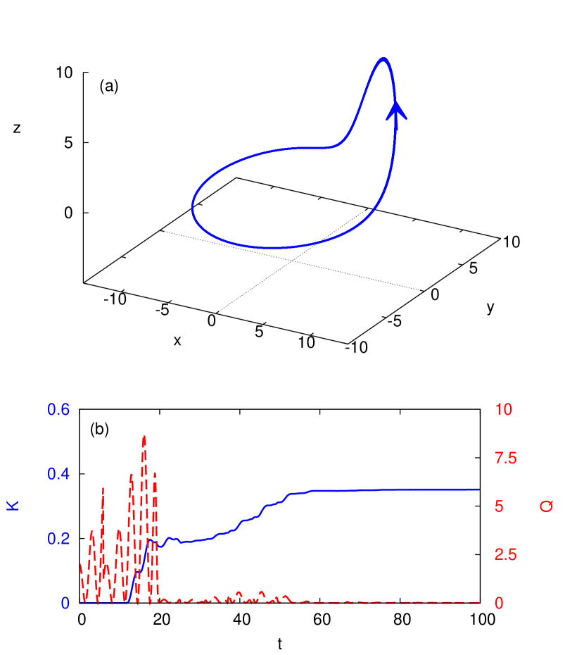
Figure 5: (Color online) Adaptive control of an unstable periodic orbit in the Rössler attractor Eq. (18). (a): Phase portrait (after a transient time of 150 time units). (b): Time series of $K(t)$ with adaptive control given by Eq. (19) as solid (blue) curve. The dashed (red) curve shows the goal function $Q$. Parameters: $a=0.2$, $b=0.2$, $\mu=6.5$, $\gamma=0.1$, $\tau=5.91679$.

In this section we apply the adaptive delayed feedback control algorithm to the Rössler system which is a paradigmatic model for chaotic systems. The system exhibits chaotic oscillations born via a cascade of period-doubling bifurcations and is given by the following equations including the control term:

$$\dot{x}(t) = -y(t)-z(t)-K[x(t)-x(t-\tau)]$$ (18a)

$$\dot{y}(t) = x(t)+ay(t)$$ (18b)

$$\dot{z}(t) = b+z(t)[x(t)-\mu].$$ (18c)

In the following, we fix the parameter values as $a=0.2$, $b=0.2$, and $\mu=6.5$ in the chaotic regime. Unstable periodic orbits with periods $T_{1}\approx 5.91679$ (”period-1 orbit”) and $T_{2}\approx 11.82814$ (”period-2 orbit”) are embedded in the chaotic attractor. As shown in Ref. BAL05, by a bifurcation analysis, application of the delayed feedback of Pyragas type with $\tau=T_{1}$ and $0.24<K<2.3$ stabilizes the period-1 orbit, and it becomes the only attractor of the system. In Ref. JUS97, it was predicted analytically by a linear expansion that control is realized only in a finite range of the values of $K$: At the lower control boundary the limit cycle should undergo a period-doubling bifurcation, and at the upper boundary a Hopf bifurcation occurs generating a stable or an unstable torus from a limit cycle (Neimark-Sacker bifurcation).

We use $Q(x)=[x(t)-x(t-\tau)]^{2}/2$ as a goal function and as in the previous Section obtain the speed-gradient adaptation algorithm for $K$ GUZ08 :

$$\dot{K}(t)=\gamma[x(t)-x(t-\tau)][x(t)-2x(t-\tau)+x(t-2\tau)]$$ (19)

with the initial value $K(0)=0$.

Figure 5(a) depicts the time series of a stabilized orbit for a time delay $\tau=T_{1}$. Panel (b) shows that the adaptation algorithm converges to an appropriate value of $K$ and the cost function tends to zero.

Contrary to the previous case, it is not possible to set the adaptation gain $\gamma$ to $1$ by rescaling the system but the value of $\gamma$ is crucial for successful control. To explore the role of $\gamma$, we determine the fraction of realizations $f_{c}$ where the control goal is reached as a function of $\gamma$. The initial conditions are Gaussian distributions with the mean $\left<x(0)\right>=\left<y(0)\right>=\left<z(0)\right>=0$, respectively, and the standard deviations are $\sigma_{x(0)}=\sigma_{y(0)}=\sigma_{z(0)}=1$. It is assumed that the control goal is reached at time $t_{c}$ if the following condition holds: $\left<Q\right>\equiv\int_{t_{c}-2\tau}^{t_{c}}Q(t^{\prime})dt^{\prime}<0.002\tau$.

Figure 6 depicts $f_{c}(\gamma)$ ((red) circles) and $t_{c}(\gamma)$ ((blue) crosses) demonstrating that the optimal adaptation gain is around $\gamma=0.26$. For $\gamma$ close to this value, the algorithm converges fast and reliably. Accordingly, the standard deviation of $t_{c}$ is small.

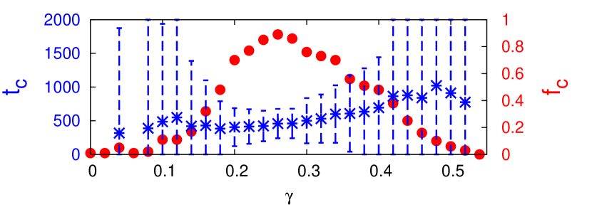
Figure 6: (Color online) Adaptive control of the Rössler system. Full (red) circles: fraction of realizations $f_{c}$ where the adaptive control algorithm stabilized the orbit versus the adaptation gain $\gamma$; black (blue) crosses: Average time $t_{c}$ after which the control goal is reached versus $\gamma$; dotted (blue) lines: error bars (standard deviation) corresponding to $t_{c}$. Other parameters as in Fig. 5. Total number of realizations: 100.

This demonstrates that for appropriate values of $\gamma$, the chaotic dynamics can be controlled.

IV Conclusion

In summary, we have proposed an adaptive controller based on the speed-gradient method, to tune the feedback gain of time-delayed feedback control to an optimal value. We have shown that the adaptation algorithm can find appropriate values for the feedback gain and thus stabilize the desired periodic orbit or fixed point. This has been realized both for the stabilization of an unstable focus in a generic model and the stabilization of an unstable periodic orbit embedded in a chaotic attractor. We have demonstrated the robustness of our method to different initial conditions and noise. We stress that this adaptive controller may especially be useful for systems with unknown or slowly changing parameters where the domains of stability in parameter space are unknown. In particular, we have shown by a simulation with a drifting bifurcation parameter $\lambda$ that our method is able to follow such slow parameter drifts. It should be noted that the automatic adjustment of the feedback gain $K$ is possible without changing the value of the adaptation gain $\gamma$ of the speed-gradient method. This shows that the algorithm is robust and simple to apply. Our method might be used to tune more than one parameter, increasing its range of possible application.

- (1) E. Ott, C. Grebogi, and J. A. Yorke, Phys. Rev. Lett. 64, 1196 (1990).
- (2) Handbook of Chaos Control, edited by E. Schöll and H. G. Schuster (Wiley-VCH, Weinheim, 2008), second completely revised and enlarged edition.
- (3) K. Pyragas, Phys. Lett. A 170, 421 (1992).
- (4) A. G. Balanov, N. B. Janson, and E. Schöll, Phys. Rev. E 71, 016222 (2005).
- (5) A. Ahlborn and U. Parlitz, Phys. Rev. Lett. 93, 264101 (2004).
- (6) M. G. Rosenblum and A. S. Pikovsky, Phys. Rev. Lett. 92, 114102 (2004).
- (7) P. Hövel and E. Schöll, Phys. Rev. E 72, 046203 (2005).
- (8) J. E. S. Socolar, D. W. Sukow, and D. J. Gauthier, Phys. Rev. E 50, 3245 (1994).
- (9) T. Dahms, P. Hövel, and E. Schöll, Phys. Rev. E 76, 056201 (2007).
- (10) M. E. Bleich and J. E. S. Socolar, Phys. Lett. A 210, 87 (1996).
- (11) W. Just, T. Bernard, M. Ostheimer, E. Reibold, and H. Benner, Phys. Rev. Lett. 78, 203 (1997).
- (12) W. Just, D. Reckwerth, J. Möckel, E. Reibold, and H. Benner, Phys. Rev. Lett. 81, 562 (1998).
- (13) K. Pyragas, Phys. Rev. Lett. 86, 2265 (2001).
- (14) S. Yanchuk, M. Wolfrum, P. Hövel, and E. Schöll, Phys. Rev. E 74, 026201 (2006).
- (15) R. Hinz, P. Hövel, and E. Schöll, Chaos 21, 023114 (2011).
- (16) N. Baba, A. Amann, E. Schöll, and W. Just, Phys. Rev. Lett. 89, 074101 (2002).
- (17) H. Nakajima, Phys. Lett. A 232, 207 (1997).
- (18) B. Fiedler, V. Flunkert, M. Georgi, P. Hövel, and E. Schöll, Phys. Rev. Lett. 98, 114101 (2007).
- (19) W. Just, B. Fiedler, V. Flunkert, M. Georgi, P. Hövel, and E. Schöll, Phys. Rev. E 76, 026210 (2007).
- (20) A. L. Fradkov, Autom. Remote Control 40, 1333 (1979).
- (21) A. L. Fradkov and A. Y. Pogromsky, Introduction to Control of Oscillations and Chaos (World Scientific, Singapore, 1998).
- (22) A. L. Fradkov, Physics-Uspekhi 48, 103 (2005).
- (23) A. L. Fradkov, Cybernetical Physics: From Control of Chaos to Quantum Control (Springer, Heidelberg, Germany, 2007).
- (24) P. Y. Guzenko, P. Hövel, V. Flunkert, A. L. Fradkov, and E. Schöll, Adaptive Tuning of Feedback Gain in Time-Delayed Feedback Control, Proc. 6th EUROMECH Nonlinear Dynamics Conference (ENOC-2008), ed. A. Fradkov, B. Andrievsky, IPACS Open Access Library http://lib.physcon.ru (e-Library of the International Physics and Control Society), 2008.
- (25) A. L. Fradkov, I. V. Miroshnik, and V. O. Nikiforov, Nonlinear and Adaptive Control of Complex Systems (Kluwer, Dordrecht, 1999).
- (26) A. Astolfi, D. Karagiannis, and R. Ortega, Nonlinear and Adaptive Control with Applications (Springer, Heidelberg, 2008).
- (27) M. Krstic, I. Kanellakopoulos, and P. Kokotovic, Nonlinear and Adaptive Control Design (Wiley, New York, 1995).
- (28) O. Beck, A. Amann, E. Schöll, J. E. S. Socolar, and W. Just, Phys. Rev. E 66, 016213 (2002).
- (29) Y. A. Astrov, A. L. Fradkov, and P. Y. Guzenko, Phys. Rev. E 77, 026201 (2008).
- (30) V. Flunkert and E. Schöll, Phys. Rev. E 84, 016214 (2011).