Direction dependent mechanical unfolding and Green Fluorescent Protein as a force sensor

Abstract

An Ising–like model of proteins is used to investigate the mechanical unfolding of the Green Fluorescent Protein along different directions. When the protein is pulled from its ends, we recover the major and minor unfolding pathways observed in experiments. Upon varying the pulling direction, we find the correct order of magnitude and ranking of the unfolding forces. Exploiting the direction dependence of the unfolding force at equilibrium, we propose a force sensor whose luminescence depends on the applied force.

I Introduction

In recent years many efforts have been devoted to the study of the mechanical properties of biopolymers under mechanical loading. Many experimental groups have studied the unfolding and refolding trajectories of proteins and nucleic acids by applying a controlled force with AFM or optical tweezers techniques bus1 ; bus2 ; Rief2004 ; Rief2006 ; EPL08 ; KumarLi2010 . These works have triggered a number of numerical investigations, where the same molecules have been studied, under conditions otherwise not accessible to the experimental techniques KumarLi2010 ; Irbaeck95 ; Rief2007 ; AlbPrlJCP07 ; PRLTorc07 ; thiruPnas08 ; AlbPrl08 ; Andrews2008 ; BiophysJ09 ; AlbPrl09 ; AlbJCP10 ; PREAlb10 .

One of the most interesting proteins studied with force spectroscopy is the Green Fluorescent protein (GFP), which exhibits bright green fluorescence when exposed to light with a suitable wavelength. GFP has many applications in biotechnology, from localization of proteins in a living cell, to metal ion or pH sensor Zimmer02 . Furthermore, such a molecule has been the subject of mechanical experiments and numerical simulations Rief2004 ; Rief2006 ; Rief2007 aimed at characterizing its response to external force and the structure of its intermediate states. The final goal of such studies is a full characterization of the GFP response to mechanical stress, so as to pave the way to its use as a molecular force sensor. Indeed, it is commonly believed that GFP fluoresces only when its structure is almost intact Dopf1996 ; Li1997 . This represents a restriction for the use of the GFP to probe forces in vivo, since a fluorescent (non-fluorescent) protein indicates that the applied force is below (above) some typical rupture force, but one cannot obtain an estimate of the actual value of the force by measuring the fluorescence. Thus in the present letter we propose a practical method to circumvent this limitation, by exploiting the fact that if pulled along different directions, the GFP exhibits different mechanical properties, and thus different rupture forces, as already observed in experiments Rief2006 . We will first introduce a model for the GFP that has already been used to evaluate the phase diagram, the free energy landscape AlbPrlJCP07 and the unfolding pathways AlbPrl08 ; AlbJCP10 of widely studied proteins and of RNA molecules AlbPrl09 . We will compare the response of the model protein to experimental outcomes, and then we will study the rupture force of the GFP when pulled along different directions. Finally, we will introduce a model polyprotein made up of different GFP modules, and we will show how such a molecule can easily provide the value of the applied force in a wide range of values, and thus be used as a force probe. To the best of our knowledge, it is the first time such a molecular device is proposed in the literature.

II The model

A native–centric, Ising–like model of protein folding VarieWSME has been generalized in previous works AlbPrlJCP07 to deal with the case of mechanical unfolding. In such a model the state of a $N$ residues long protein is determined by two sets of binary variables: the variables $m_{k}$ are associated to each residue being $1$ or $0$ according to whether the residue is native–like or not, and the variables $\sigma_{ij}=\pm 1$ give the orientation (parallel or antiparallel to the external force) of a native–like stretch delimited by residues $i$ and $j>i$ in a non–native state, such that $S_{ij}=(1-m_{i})(1-m_{j})\prod_{k=i+1}^{j-1}m_{k}$. A negative interaction energy $h_{ij}$ is associated to two residues $i$ and $j$ if they are in contact in the native structure and if they are in the same native stretch. The corresponding hamiltonian is

$$H(\left\{{m}\right\},\left\{{\sigma}\right\})=\sum_{i=1}^{N-1}\sum_{j=i+1}^{N}h_{ij}\prod_{k=i}^{j}m_{k}+U(L(\left\{{m}\right\},\left\{{\sigma}\right\})),$$ (1)

where $L=\displaystyle{\sum_{i=a}^{b-1}\sum_{j=i+1}^{b}l_{ij}\sigma_{ij}S_{ij}}$ is the molecule elongation (distance between the $C_{\alpha}$ atoms of the two residues $a$ and $b$ where force is applied, $1\leq a<b\leq N$), $l_{ij}$ is the native distance between $C_{\alpha}$ atoms of residues $i$ and $j$, and $U(L(\left\{{m}\right\},\left\{{\sigma}\right\}))$ is the term describing the coupling to the external force, which depends on the pulling protocol. In the case of a constant force the energy reads $U=-fL$. In the case of a constant velocity protocol the force is applied through a harmonic potential whose center moves at constant velocity, and the corresponding energy is $U=k/2(L-vt)^{2}$.

Under a constant force the equilibrium thermodynamics of the model is exactly solvable AlbPrlJCP07 , while for the study of the kinetics we resort to Monte Carlo simulations.

Before studying the molecule response to external forces, it is interesting to consider the free energy profile at zero force. More specifically, we have computed the free energy profile as a function of the fraction of native residues $M$ (Fig. 1) and contacts $Q$ (Fig. 2) at the denaturation temperature. Inspection of these plots indicates that at this temperature: (i) when the protein is in its native state, all the native contacts are formed, and almost all the residues are in the native configuration; (ii) in the unfolded state, no native contacts are formed, and 1/3 of the residues are in the native configuration; (iii) the transition state corresponds to $Q\sim 0.3\div 0.4$, while at $Q\sim 0.5\div 0.7$ there are some hints of the possible existence of intermediate states; (iv) the unfolding barrier is of the order of 25 $k_{B}T$ in both cases. Our results for the free energy profile as a function of $Q$ can be compared to the result obtained in Andrews2008 by weighted–histogram analysis of molecular dynamics (MD) data. The qualitative picture is very similar, although some differences can be observed. The MD result show that some fluctuations in native contacts are allowed in both the native and unfolded states, a feature which is missing in our result due to the extreme cooperativity of the model. Moreover, the unfolding barrier is predicted by MD to be around 15 $k_{B}T$: this is consistent with the observation that our model predicts systematically higher energy barriers and unfolding forces (see discussion below).

Figure 1: Free energy profile $\Delta G$, as a function of the fraction of native residues $M$, at unfolding temperature $T=356$ K and zero force.

Figure 2: Free energy profile $\Delta G$, as a function of the fraction of native contacts $Q$, at unfolding temperature $T=356$ K and zero force.

From now on we set the temperature at $T=293$ K. The native structure of GFP is basically a $\beta$–barrel made of 11 $\beta$-strands, with a N-terminal $\alpha$–helix.

In Fig. 3 the free energy profile $\Delta G(L)$ is reported for a typical case, where the equilibrium unfolding force $f=35.9$ pN is applied to the molecule ends. Besides the native and the unfolded minima we can see three other local minima (or bends which become actual minima at different values of the force) around $11$, $18$ and $25$ nm. As will be shown in detail in the next section, these local minima and bends correspond to intermediate states effectively populated in the simulations. Analysing the equilibrium probability $0\leq\langle m_{k}(L)\rangle\leq 1$ that the $k-$th residue is native–like when the molecule total elongation is $L$ (data not shown), we find out that such bends correspond to the following structures: $\beta_{1}$ and $\beta_{11}$ (for $L\simeq 11$ nm), $\beta_{10}\beta_{11}$ (18 nm) and $\beta_{1}\beta_{2}\beta_{3}$ (25 nm). Here and in the following, $\beta_{k}\cdots\beta_{n}$ denotes an unfolded structure of the GFP, where $\beta$–strands from $k$ to $n$ are not in a native–like conformation, i.e. they are unfolded (in all these structures the N–terminal $\alpha$–helix is also not in a native–like conformation).

Figure 3: Free energy profile $\Delta G$ as a function of the protein elongation $L$, with $T=293$ K, and force $f=35.9$ pN applied to the molecule ends.

III Simulations and comparison with experiments

We first consider simulations at constant velocity, mimicking the effect of an AFM cantilever, which is retracted at a velocity $v$. The force is applied to the molecule ends and we set $k=30$ pN/nm and consider velocities $v=0.3$, $1$ $\mu$m/s, $2$ $\mu$m/s and $3.6$ $\mu$m/s. In ref. Rief2007 it was found that the most likely unfolding pathway is $\alpha\rightarrow\beta_{1}\rightarrow\beta_{2}\beta_{3}$ (the $\alpha$–helix unfolds first, then $\beta$–strand 1, then strands 2 and 3 simultaneously, then the rest of the protein), observed in 72% of the trajectories at $v=2.5$ $\mu$m/s. A different pathway, $\alpha\rightarrow\beta_{11}$, was observed in the remaining 28% of the trajectories.

The N–terminal $\alpha$–helix is the first secondary structure element to unravel in both pathways. This event is typically associated to very small signals, almost masked by fluctuations, at odds with the clear jumps we observe in the end–to–end length for the detaching of $\beta$–strands (see fig. 4). This is analogous to what occurs in the experiments where the unfolding of the helix is associated to a very smooth “hump–like” transition with a short contour length increase of $3.2$ nm in the force-extension traces in Rief2004 and by a small jump in the root mean square distance as a function of time in Rief2007 .

We have found that, at all velocities considered, in less than 10% of the trajectories $\beta_{11}$ is the first strand to unravel, while the remaining trajectories follow the major unfolding pathway found in experiments. In Fig. 4, we plot a typical unfolding trajectory of our GFP model when the force is applied to the molecule ends. In particular, we plot, as functions of time, the end–to–end length $L$, the force and several weighted fractions of contacts between adjacent $\beta$-strands $\phi_{\beta_{i-j}}$, giving the fraction of native contacts between the strands $\beta_{i}$ and $\beta_{j}$, see AlbJCP10 .

Major unfolding pathway.

Inspection of the top panel of Fig. 4, corresponding to the major unfolding pathway, provides clear evidence that there are three main unfolding events. (i) A drop in the number of contacts between strands 1 and 2, signalling the unfolding of $\beta_{1}$ (actually the $\alpha$–helix has already unfolded, as discussed above, but the corresponding fraction of native contacts $\phi_{\alpha}$ is not reported in the figure for the sake of clarity). The length of the corresponding intermediate state is in the range $10\div 12.5$ nm, where the free energy profile $\Delta G(L)$ shows a bend, see fig. 3. (ii) A drop in the number of contacts involving strands 2 and 3, signalling the unfolding of these strands. The corresponding intermediate length is around 20 nm, where the free energy profile $\Delta G(L)$ has a local minimum. (iii) A drop in the number of contacts involving strands 10 and 11, signalling the unfolding of these strands. The corresponding intermediate length is in the range $30\div 37$ nm: inspection of fig. 3 suggests that for such an elongation the molecules lies in the basin of the unfolded minimum.

Minor unfolding pathway.

The bottom panel of Fig. 4 corresponds to the minor unfolding pathway and we can see that the first strand to unravel is $\beta_{11}$ followed by $\beta_{10}$. In Rief2007 the unfolding pathway was only traced up to the $\Delta\beta_{11}$ intermediate because the subsequent event is the flattening of the barrel but, after the barrel flattens, there is at least another rupture event as the last force jump in Fig. 1b of Rief2007 shows. It is reasonable to assume that this event is related to the breaking of native-like contacts between the beta strands, which were not ruptured during the flattening of the barrel. Our model, which lacks a fully three-dimensional representation, cannot describe the flattening of the barrel, while it can describe with a high time resolution the breaking of the beta strand contacts, which here yield in a few distinct steps (Fig. 4, bottom panel).

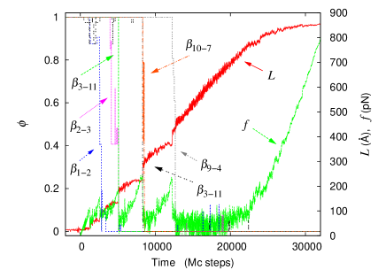
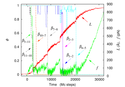
Figure 4: (color online) Typical unfolding trajectories of a GFP module under constant velocity pulling ($v=0.3\ \mu$m/s). Length $L$, force $f$ and weighted fractions $\phi_{\beta_{i-j}}$ of strand–strand contacts as functions of time for two typical cases: major (top panel) and minor (bottom panel) unfolding pathway, see text.

We can now put the local minima and bends of the free energy landscape of Fig. 3 (which is a thermodynamic equilibrium property of the system) in correspondence with intermediates found in our simulations and in experiments (which are performed in non-equilibrium conditions). Some of these features of the free energy profile are indeed barely visible, but the equilibrium probabilities $\langle m_{k}(L)\rangle$, we introduced in the previous section to give a structural interpretation of the various minima and bends, are perfectly consistent with the nonequilibrium $m_{k}$ values obtained from the simulations, which allow us to identify the structures of the nonequilibrium intermediates.

In ref. Rief2004 the authors observed two intermediates with separation values from native configuration of $3.2$ and $10$ nm. The first one, is an intermediate with only the N–terminal $\alpha$–helix detached that profile of Fig. 3 does not show, while the second is an intermediate with the N–terminal $\alpha$–helix detached and a $\beta$–strand detached which corresponds to the bend at $11$ nm ($9.2$ nm away from native state) in Fig. 3. The authors of ref. Rief2007 report the existence of another intermediate (N–terminal $\alpha$–helix and first, second and third $\beta$–strands detached) with a distance of $26.3$ nm from the native state($16.3$ nm from the previous second intermediate) which is clearly associated to our dip at $25$ nm. The $18$ nm intermediate has no analogue in experiments.

Different directions.

We now consider simulations where the points of force application are not the molecule ends, so that the direction of the force with respect to the molecule is varied. Table 1 reports, for different directions (specified through the application point residue numbers), the mean unfolding forces, where unfolding is defined as unravelling of the first $\beta$ strand. Since most of these directions were considered in experiments Rief2006 , at least at $v=3.6\ \mu$m/s, it is interesting to compare our results to the experimental ones. Our unfolding forces are systematically larger than the experimental values, with the largest discrepancies (a factor 2 to 3) occurring for directions 3–212 and 132–212. However, it is interesting that in spite of the simplicity of the model, which lacks a fully three-dimensional representation, the orders of magnitude for the rupture forces are correct and many qualitative aspects are reproduced. In particular, by analyzing the experimental data one finds that the unfolding force increases with the following order: (i) pulling along the end–to–end direction (it must be noted that the rupture force along this direction was measured for $v=0.3\ \mu$m/s instead of $3.6\ \mu$m/s as most other directions); (ii) pulling along the 3–212 and 132–212 directions, the corresponding rupture forces are equal within the experimental error; (iii) pulling along the 182–212 and 3–132 directions, the corresponding rupture forces are equal within the experimental error (though the latter was measured for $v=2\ \mu$m/s); (iv) pulling along the 117–182 direction. This hierarchy is respected by our results: we find that the rupture force increases when we consider the pulling directions as ordered above, the only exception being for 3–212 and 132–212, whose unfolding forces are not equal (we obtain a smaller force for the latter), and the same holds for 182–212 and 3–132 (we obtain a larger force for the latter).

Table 1: Unfolding forces at different velocities for different directions. Experimental values (^∗ from ref. Rief2004 and ^† from ref. Rief2006 ) in parentheses.

	Unfolding force (pN)
Direction	$v=0.3\ \mu$m/s	$v=2\ \mu$m/s	$v=3.6\ \mu$m/s
end–end	$140\pm 3$ ($104\pm 40$)∗	$177\pm 7$	$184\pm 13$
182–end	$196\pm 7$	$226\pm 6$	$244\pm 7$
3–212	$244\pm 12$	$298\pm 12$	$317\pm 20$ ($117\pm 19$)†
132–212	$251\pm 7$	$266\pm 3$	$273\pm 6$ ($127\pm 23$)†
132–end	$306\pm 12$	$360\pm 20$	$381\pm 26$
182–212	$365\pm 2$	$390\pm 7$	$409\pm 15$ ($356\pm 61$)†
3–132	$383\pm 16$	$471\pm 49$ ($346\pm 46$)†	$535\pm 80$
117–182	$467\pm 3$	$501\pm 11$	$512\pm 11$ ($548\pm 57$)†

Finally, in Table 2 we report the potential width values $x_{u}$ corresponding to the rupture of the first $\beta$–strand for different directions. These were obtained through a fit of the most probable unfolding force $f_{M}$ as a function of velocity to the Evans–Ritchie theory Evans1997 ; Evans1999 , which gives

$$f_{M}=\frac{k_{B}T}{x_{u}}\ln\left(\frac{\tau_{0}x_{u}}{k_{B}T}r\right)$$ (2)

where $\tau_{0}$ is the unfolding time at zero force. It must be kept in mind that in the Evans–Ritchie theory the force grows with a constant rate $r=k\cdot v$ and hence its applicability to the present case (harmonic potential whose center moves at constant velocity $v$) is only approximate.

Table 2: Potential width $x_{u}$ obtained from a fit to Eq. 2. Experimental values between parentheses.

direction	$x_{u}$ (nm)	direction	$x_{u}$ (nm)
end–end	$0.21\pm 0.04$ ($0.28\pm 0.03$)	132–end	$0.14\pm 0.01$
182–end	$0.22\pm 0.03$	182–212	$0.24\pm 0.04$ ($0.14\pm 0.002$)
3–212	$0.14\pm 0.01$ ($0.45\pm 0.01$)	3–132	$0.11\pm 0.03$ ($0.125\pm 0.005$)
132–212	$0.46\pm 0.06$ ($0.32\pm 0.005$)	117–182	$0.22\pm 0.01$ ($0.12\pm 0.003$)

Our potential widths are consistent with experimental ones only in a few cases (end–end, 3–132): once again, this might be attributed to the fact that our model lacks a fully three–dimensional representation.

It must also be observed that the Evans–Ritchie theory is built on the assumption that $x_{u}$ is independent of the applied force, and this can be another source of error in the determination of $x_{u}$. This assumption was relaxed in more recent theories Dudko ; Paci which yield generalizations of Eq. 2, which predict that the $f_{M}$ vs $\ln v$ plot is nonlinear, with the slope being an increasing function of $v$, as observed in many experiments. Indeed our data show some nonlinearity, but this is too small to apply these theories, probably because our velocities span only 1 order of magnitude. Previous applications of these theories Dudko ; AlbPrlJCP07 ; Paci were done on data sets with velocities spanning 4–5 orders of magnitude, such that the nonlinear effects were much more important, but such a wide range of velocities is beyond the scope of the present paper.

IV GFP polyprotein

As we discussed above, the equilibrium properties of the GFP at constant force, can be obtained exactly, for any pulling direction. Exploiting this result, we study a polyprotein where each module is connected to the neighbouring ones through different points of force application, as illustrated in Fig. 5.

\psfrag{f}[ct][ct][1.]{$f$}\includegraphics[width=227.62204pt]{multi_gfp1.eps}

Figure 5: (color online) Sketch of a polyprotein made of various modules connected between them through different residues.

For example Dietz et al. Rief2006 already proposed a copolymer with mixed linkage geometries GFP(3,212)(132,212), made up of several GFP modules, where a module linked by its (3,212) residues to the main structure was alternated with a module linked by its (132,212) residues. Such a molecule can be easily obtained by using the cysteine engineering method discussed in ref. RiefProt , which allows one to construct polyproteins with precisely controlled linkage topologies: the points of force application to each module correspond to the position of the linking cysteines in the folded tertiary structure. In order to understand the general behavior of our model polyprotein under a constant force we first investigate the response to a constant force of a single GFP module. The corresponding unfolding forces are reported in Table 3.

Table 3: Equilibrium unfolding force for different directions.

direction	unfolding force (pN)	direction	unfolding force (pN)
end–end	$35.9$	182–end	$65.0$
3–212	$38.9$	117–190	$67.3$
3–182	$42.6$	102–190	$71.2$
117–end	$50.8$	117–182	$78.1$
3–132	$56.4$	132–182	$96.7$

We then proceed by studying the response to a constant force of a polyprotein made up of 10 modules, each with different linkage topologies. It is worth to note that at equilibrium a force applied to the free ends of the polyproteins will have the same value throughout the whole chain. Thus, the different modules will unfold at different values of the force, according to the hierarchy shown in Tab. 3, and thus the luminescence will be different for different values of the force. If we assign a value 1 (in an arbitrary scale) to the maximum possible luminescence, where each module is emitting green light, a luminescence of 0.5 will correspond to a configuration, and thus to a force, where half of the modules are unfolded (non intact structure). Given that each module with a different linkage has a different unfolding force, we obtain a curve like the one shown in fig. 6, relating the luminescence of the polyprotein to the force applied to its free ends, where the force ranges from 35.9 to 96.7 pN, see Table 3. It is worth to note that interface interactions and aggregation effects between neighbouring units in polyproteins similar to the one we propose, have been ruled out by experimental investigations, see Rief2006 .

Figure 6: Fraction of native–like modules as a function of force at $T=$293 K. Each “step” corresponds to the unfolding of a different module in the polyprotein and thus to a decrease in the luminescence by a “unit”.

Figure 6 represents an important result of this paper. It is worth to note that more modules, with different linkages, can be added, and this would give a more precise determination of the force. Once the polyprotein we propose has been engineered, a curve like the one shown in fig. 6 can be very easily obtained in an optical tweezers experiment at constant force as those discussed, e.g., in ref. bus1 . This approach would also allow one to calibrate the device. Finally, we want to emphasize that, although unfolding studies of GFP along different directions where already performed in, e.g., Rief2006 ; Rief2007 , those previous studies considered the dynamic-loading set up, with a constant retraction speed of the AFM cantilever. On the contrary we investigate here for the first time the unfolding at constant force of GFP. The unfolding force of a molecule under dynamic loading depends not only on the molecular features, but also on the force rate, and thus a force probe based on those data must be able to measure at the same time the loading rate and the rupture force. Our constant force probe does not exhibit this drawback.

V Conclusions

The Ising–like model of protein mechanical unfolding describes correctly the most important qualitative aspects of the direction–dependent mechanical unfolding of the Green Fluorescent Protein, namely the unfolding pathways and intermediates observed when pulling at constant velocity from the molecule ends, and the orders of magnitude and ranking of the unfolding forces corresponding to different directions. Some features, like the flattening of the barrel or the potential widths corresponding to many directions, cannot however be described by our model, which lacks a fully three–dimensional representation. Moreover, from a more quantitative point of view, our energy barriers and unfolding forces are systematically larger than those observed in experiments.

We have exploit the dependence of the unfolding force on the pulling direction to investigate a force sensor based on a GFP polyprotein where each module is linked with a different geometry to the nearest neighbouring modules, so as to experience the force along different direction, yielding a device whose luminescence depends (in a discrete way) on the force. It is worth noting that such a device may be used in in-vivo experiments, to measure forces at molecular level, e.g. inside cells, in a non–invasive way.

- (1) J. Liphardt et al, Science 292, 733 (2001)
- (2) B. Onoa et al, Science 299, 1892 (2003)
- (3) H. Dietz and M. Rief, Proc. Natl. Acad. Sci. USA 101, 16192 (2004)
- (4) H. Dietz, F. Berkemeier, M. Bertz, and M. Rief, Proc. Natl. Acad. Sci. USA 103, 12724 (2006)
- (5) A. Imparato, F. Sbrana, M. Vassalli, Europhys. Lett. 82, 58006 (2008).
- (6) S. Kumar and M. S. Li, Phys. Rep. 486, 1 (2010)
- (7) A. Irbäch, S. Mitternacht, and S. Mohanty, Proc. Natl. Acad. Sci. U.S.A. 102, 13427 (2005)
- (8) M. Mickler, R. Dima, H. Dietz, C. Hyeon, D. Thirumalai, and M. Rief, Proc. Natl. Acad. Sci. USA 104, 20268 (2007)
- (9) A. Imparato, A. Pelizzola and M. Zamparo, Phys. Rev. Lett. 98, 148102 (2007); A. Imparato, A. Pelizzola and M. Zamparo, J. Chem. Phys. 127, 145105 (2007).
- (10) A. Imparato, S. Luccioli, A. Torcini, Phys. Rev. Lett. 99, 168101 (2007).
- (11) B.T. Andrews, S. Gosavi, J.M. Finke, P.A. Jennings, Proc. Natl. Acad. Sci. USA 105, 12283 (2008)
- (12) C. Hyeon, G. Morrison, and D. Thirumalai, Proc. Natl. Acad. Sci. U.S.A. 105, 9604 (2008)
- (13) A. Imparato and A. Pelizzola, Phys. Rev. Lett. 100, 158104 (2008)
- (14) S. Mitternacht, S. Luccioli, A. Torcini, A. Imparato, A. Irbäck, Biophys. J. 96, 429 (2009).
- (15) A. Imparato, A. Pelizzola, and M. Zamparo, Phys. Rev. Lett. 103, 188102 (2009)
- (16) M. Caraglio, A. Imparato, and A. Pelizzola, J. Chem. Phys. 133, 065101 (2010)
- (17) S. Luccioli, A. Imparato, S. Mitternacht, A. Irbäck and A. Torcini, Phys. Rev. E 81, 010902 (2010).
- (18) M. Zimmer, Chem. Rev. 102, 759 (2002)
- (19) J. Dopf and T. M. Horiagon, Gene 173, 39 (1996)
- (20) X. Li, G. Zhang, N. Ngo, X. Zhao, S. Kain, and C. C. Huang, Biol. Chem. 272, 28545 (1997)
- (21) E. Evans and K. Ritchie, Biophys. J. 72, 1541 (1997)
- (22) E. Evans and K. Ritchie, Biophys. J. 76, 2439 (1999)
- (23) H. Wako and N. Saitô, J. Phys. Soc. Jpn 44, 1931 (1978); H. Wako and N. Saitô, ibid. 44, 1939 (1978); V. Muñoz et al., Nature 390, 196 (1997); V. Muñoz et al. Proc. Natl. Acad. Sci. USA 95, 5872 (1998); V. Muñoz and W.A. Eaton, ibid. 96, 11311 (1999); P. Bruscolini and A. Pelizzola, Phys. Rev. Lett. 88, 258101 (2002).
- (24) O. K. Dudko, A. E. Filippov, J. Klafter, and M. Urbakh, Proc. Natl. Acad. Sci. U.S.A. 100, 11378 (2003); O. K. Dudko, G. Hummer, and A. Szabo, Phys. Rev. Lett. 96, 108101 (2006).
- (25) M. Schlierf, Z.T. Yew, M. Rief and E. Paci, Biophys. J. 99, 1620 (2010).
- (26) H. Dietz, M. Bertz, M. Schlierf, F. Berkemeier, T. Bornschlögl, J. P. Junker, and M. Rief, Nat. Protocols 1, 80 (2007)