Abstract
The usual power function error estimates do not capture the true order of uniform accuracy for thin plate spline interpolation to smooth data functions in one variable. In this paper we propose a new type of power function and we show, through numerical experiments, that the error estimate based upon it does match the expected order. We also study the relationship between the new power function and the Peano kernel for univariate thin plate spline interpolation.
1 Introduction
For each , define the basis function by
Let be the integer part of . For any integer and any set of values of a target function prescribed at the set of equi-spaced knots , where , Micchelli’s theory [7] of conditionally positive definite radial basis functions guarantees the existence of a unique function of the form
| (1.1) |
that satisfies the interpolation conditions
| (1.2) |
as well as the ‘side’ conditions
| (1.3) |
In this paper we focus on the special case corresponding to the thin plate spline (TPS) basis function and we investigate the rate at which the interpolant (1.1) converges to uniformly over , as . If has a Lipschitz continuous third derivative on , Bejancu [3] proved that the uniform error over a fixed compact subset of inherits the maximal convergence rate obtained by Powell [9] and Buhmann [5] for ‘cardinal’ TPS interpolation on the infinite grid . Due to boundary effects, however, the uniform norm of the error over the full interval decays at the much slower rate , as illustrated numerically in [2, 11, 6]. The usual method for error estimation in radial basis function interpolation, reviewed in the next section, delivers bounds of the form
where is the so-called ‘power function’ associated with , while belongs to the ‘native space’ generated by [15, 17]. It is well known that theoretical convergence rates based upon bounding uniformly for do not match the actual rates of decay of the error achieved in numerical experiments if has sufficiently many continuous derivatives. This discrepancy was first observed by Powell [10] for the bivariate TPS interpolant. For , in section 3, we obtain a new error bound which employs a ‘mixed power function’ defined by means of the basis functions and , for . We then perform a numerical study of as , which shows that, for , the mixed power function decays like a constant multiple of . This matches exactly the previously known numerical order of uniform convergence of the error on , for sufficiently smooth target functions . In section 4 we prove that, for and , the mixed power function value is, up to a constant factor, the -norm of the Peano kernel of the error functional at . Moreover, we provide numerical evidence that the smaller -norm of this Peano kernel does not in fact decay faster than the mixed power function when measured uniformly over . It is hoped that these results and the conjectures formulated in the paper will motivate future work to establish theoretically the uniform convergence order for univariate TPS interpolation to sufficiently smooth target functions.
2 Error estimates via the standard power function
In this section we review the power function technique to obtain error estimates for univariate interpolation with the radial basis function . A key role in this technique is played by the generalized or distributional Fourier transform of . Lemma 2.1. [15, section 8.3] For each , the generalized Fourier transform of satisfies
for some constant such that .
2.1 The standard power function
As above, let , and For each which is not in the knot-set , Micchelli’s theory implies that the quadratic form
| (2.1) |
is strictly positive whenever the non-zero vector satisfies
| (2.2) |
Further, for each let be the unique function of the type (1.1)–(1.3) which satisfies the Lagrange interpolation conditions
Then we have the Lagrange representation formula for the interpolant (1.1):
| (2.3) |
as well as the reproduction formula
| (2.4) |
Proposition 2.2. [17] With the above notations, for each , the vector
has the property that it minimizes the quadratic form (2.1) among all non-zero vectors that satisfy (2.2). The minimum value of the quadratic form defines the square of the so-called ‘power function’ , namely
| (2.5) |
Note that , . Proposition 2.3. [17] For each , let
| (2.6) |
Then we have the absolutely convergent integral representation
| (2.7) |
2.2 Error estimates
For each , let be the least integer that is greater than or equal to . In order to obtain error bounds for any target function , we construct an extension of as follows (cf. [3]). By the Whitney extension theorem [16], there exists such that , for . Let be an infinitely differentiable cut-off function which satisfies for and for sufficiently large , and set
Clearly is compactly supported and coincides with on . Furthermore, its Fourier transform , defined as the continuous function
satisfies
| (2.8) |
for any . In particular, is integrable over , so can be recovered via the Fourier inversion formula
| (2.9) |
Next, let in (1.2) for . Then (2.9) and (2.3) imply the error representation
| (2.10) |
where is given by (2.6). Moreover, as a consequence of (2.8) and the definition of , we have
i.e., belongs to the so-called ‘native space’ generated by . Using (2.7) and the Cauchy-Schwarz inequality in (2.10), we obtain the error bound
| (2.11) |
Further, Wu and Schaback [17] showed that the variational characterization of the power function given in Proposition 2.1 implies
| (2.12) |
for a constant independent of . On the other hand, Schaback and Wendland [14] proved that the exponent cannot be increased in the above bound. Thus, the power function technique leads to the maximal estimate for the uniform norm of the error over .
3 A mixed power function for univariate TPS
In this section we focus on the TPS basis function , i.e. . According to (2.12), in this case the power function satisfies
However, numerical experiments [2, 6, 11] suggest that the uniform error
| (3.1) |
is of the magnitude of for a sufficiently smooth target function . To address this discrepancy, we start from the integral representation (2.7):
| (3.2) |
Note that expression (2.6) satisfies
| (3.3) |
for each fixed and Indeed, since , by (2.4) we have
| (3.4) |
This fact, together with the series expansion of the exponential, provides the bound (3.3) for . The bound for follows from the triangle inequality. As a consequence of (3.3), the integral (3.2) is still well defined if is replaced by , for any , . We may thus define the mixed power function whose square is given by
| (3.5) |
Under this integral, the Lagrange functions entering in expression (2.6) of (and generated by the TPS basis function ) are combined with the generalized Fourier transform of the basis function (cf. Lemma 2). We now let , and, as in subsection 2.2, consider the compactly supported extension of to the whole real axis. Then the error analysis of subsection 2.2 recast in terms of the mixed power function implies
| (3.6) |
where
| (3.7) |
This shows that, for a fixed , estimates of the decay of the mixed power function as will deliver error estimates for TPS interpolation. Therefore we state the following problem: Problem 3.1. Given , , does there exist an algebraic decay rate of the mixed power function uniformly over , i.e., a largest value such that
| (3.8) |
Before embarking on a numerical answer to this problem, a few remarks are in order. Firstly, note that, due to (3.7), the above target function has its compactly supported extension in the native space generated by the basis function , rather than the native space generated by the TPS basis function as in the standard estimate (2.11) for . Thus, for a given the resulting mixed power function error bound (3.6) is precisely what we would expect if we measured the TPS interpolation error for target functions in the native space of this approach is investigated in [12] in the context of approximation rather than interpolation. In particular, the mixed power function bound (3.6) applies to the smooth () target functions employed in the numerical experiments of [2, 6, 11]. Secondly, recall the two equivalent expressions for the standard power function: the direct form (2.5) and the integral representation (2.7). Letting , an application of Theorem 3 from [17] shows that the mixed power function can also be expressed as
| (3.9) | ||||
Thirdly, note that (3.4) implies that the TPS Lagrange functions satisfy constraint (2.2) of the variational problem from Proposition 2.1 with in place of . However, the solution to that problem is provided by the values of the Lagrange functions generated by interpolation with the basis function . As a result, the bounding technique [17] that leads to the estimate (2.12) for the standard power function cannot be applied to obtain estimates on . We now turn to a numerical investigation of the behaviour of the mixed power function. For a fixed parameter , , we compute an approximation of the left-hand side of (3.8) for , starting from and proceeding as follows:
- 1.
-
2.
Use (3.9) to evaluate the mixed power function at the set of mid-points and determine its maximum value
-
3.
Double and repeat steps 1–2 as long as .
The results displayed in Tables 1–4 show that, for each chosen , the values of satisfy
where and are also included in the tables. On the basis of these numerical results, we are led to the following conjecture.
| 128 | 4.774E-01 | 0.167 | 1.768E-01 | 0.333 | 6.342E-02 | 0.500 |
|---|---|---|---|---|---|---|
| 256 | 4.253E-01 | 0.167 | 1.404E-01 | 0.333 | 4.485E-02 | 0.500 |
| 512 | 3.789E-01 | 0.167 | 1.114E-01 | 0.333 | 3.171E-02 | 0.500 |
| 1024 | 3.376E-01 | 0.167 | 8.842E-02 | 0.333 | 2.242E-02 | 0.500 |
| 2048 | 3.007E-01 | 0.167 | 7.018E-02 | 0.333 | 1.586E-02 | 0.500 |
| 1.072 | 0.8912 | 0.7175 | ||||
| 128 | 2.143E-02 | 0.667 | 6.258E-03 | 0.833 |
|---|---|---|---|---|
| 256 | 1.350E-02 | 0.667 | 3.512E-03 | 0.833 |
| 512 | 8.503E-03 | 0.667 | 1.971E-03 | 0.833 |
| 1024 | 5.356E-03 | 0.667 | 1.106E-03 | 0.833 |
| 2048 | 3.374E-03 | 0.667 | 6.208E-04 | 0.833 |
| 0.5442 | 0.3568 | |||
| 128 | 1.061E-03 | 1.167 | 6.221E-04 | 1.334 | 3.327E-04 | 1.507 |
|---|---|---|---|---|---|---|
| 256 | 4.727E-04 | 1.167 | 2.473E-04 | 1.334 | 1.196E-04 | 1.503 |
| 512 | 2.106E-04 | 1.167 | 9.828E-05 | 1.333 | 4.296E-05 | 1.500 |
| 1024 | 9.381E-05 | 1.167 | 3.905E-05 | 1.333 | 1.543E-05 | 1.498 |
| 2048 | 4.179E-05 | 1.167 | 1.551E-05 | 1.333 | 5.534E-06 | 1.496 |
| 0.3049 | 0.4024 | 0.4975 | ||||
| 128 | 2.032E-04 | 1.491 | 1.661E-04 | 1.497 |
|---|---|---|---|---|
| 256 | 6.995E-05 | 1.497 | 5.808E-05 | 1.499 |
| 512 | 2.419E-05 | 1.501 | 2.039E-05 | 1.500 |
| 1024 | 8.402E-06 | 1.503 | 7.182E-06 | 1.501 |
| 2048 | 2.919E-06 | 1.505 | 2.523E-06 | 1.502 |
| 0.2814 | 0.2368 | |||
Conjecture 3.2. The mixed power function satisfies the estimate (3.8) with the algebraic decay rate
4 The mixed power function for
Note that if Conjecture 3 can be established for a particular value , then the mixed power function bound (3.6) implies a new and improved error estimate for thin plate spline interpolation on the unit interval, namely, for any ,
| (4.1) |
This would provide a theoretical explanation of the numerical results reported in [2, 6, 11]. In this section, we investigate Conjecture 3 for the special case . By (3.5) and (3.9), the square of the mixed power function , combining TPS Lagrange functions with the cubic basis function , is given by
| (4.2) | ||||
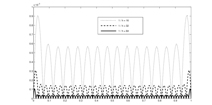
Figure 1 illustrates the decay of as . It can be confirmed numerically that the decay rate of suggested by Table 3 applies uniformly on , i.e. all peaks of the plot decay at this rate. We now relate the mixed power function to a classical error analysis method, namely the Peano kernel representation. Let
For each , is a continuous linear functional on with the usual max norm, and (3.4) implies that the linear polynomials are in the null space of . Then, for any with an absolutely continuous first derivative on , Peano’s theorem [8, p. 271] implies
| (4.3) |
where is the ‘Peano kernel’ given by
Proposition 4.1. For each , the mixed power function value is a constant multiple of the -norm of the Peano kernel .
Proof.
The reproduction property (3.4) implies that is compactly supported on , and that
Then, by Lemma 2, the Fourier transform of the kernel is the analytic and square integrable function
where is defined by (2.6). Therefore, using the first line of (4.2), the Parseval-Plancherel formula, and the compact support of , we deduce
which is the required conclusion. ∎
As a consequence, we obtain an alternative way of bounding the error in terms of the mixed power function , by using Cauchy-Schwarz directly in the right-hand side of the Peano formula (4.3). The resulting bound applies to any with an absolutely continuous first derivative on and . This represents an improvement over (3.6)–(3.7), which required for . Finally, a related question of interest is whether a sharper uniform error bound can be obtained from (4.3) via Hölder’s inequality
where and
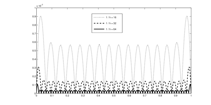
We note that this technique was used by Atkinson [1] in the late 1960s to investigate the error behavior of natural cubic spline interpolant near the endpoints of the unit interval; see also Schaback [13] for a treatment that is closer to our presentation. In the case of the TPS interpolant, a numerical answer to the question is provided in Table 5, whose entries satisfy
i.e., decays approximately with the rate near the endpoints of and this rate improves to near the midpoint. Also, Figure 2 shows that the extreme peak value is well approximated by , while all of the lower peaks decay at the faster rate. Therefore estimating the -norm of the Peano kernel leads to the same rate of decay of the uniform error (3.1) as that predicted in (4.1) by the mixed power function . We conclude the paper by remarking that any theoretical proof of the uniform decay rate of or for will have to rely on specific properties of the TPS Lagrange functions , . A potentially useful such property is the special case of [4, Theorem 3.1] stating that the Lebesgue-type constant
admits an upper bound independently of the mesh-size . It remains an open question whether this or other properties of the TPS Lagrange functions can lead to further progress on the above conjectures.
| 64 | 1.024E-04 | 1.491 | 3.633E-05 | 2.001 |
|---|---|---|---|---|
| 128 | 3.533E-05 | 1.498 | 9.098E-06 | 2.001 |
| 256 | 1.228E-05 | 1.501 | 2.293E-06 | 1.999 |
| 512 | 4.289E-06 | 1.503 | 5.694E-07 | 2.000 |
| 1024 | 1.502E-06 | 1.504 | 1.434E-07 | 1.999 |
Acknowledgements. A.B. is grateful to Michael Johnson (Kuwait University) for a suggestion which improved the presentation of the numerical results and for spotting a fallacious argument in a tentative proof of Conjecture 3 for . The final version has also benefited from the referees’ suggestions.
References
- [1] K. E. Atkinson, On the Order of Convergence of Natural Cubic Spline Interpolation, SIAM Journal on Numerical Analysis, 5 No.1 (1969), 89–101.
- [2] A. Bejancu, Convergence Properties of Surface Spline Interpolation, Ph.D. Dissertation, University of Cambridge, (1999).
- [3] A. Bejancu, Local accuracy for radial basis function interpolation on finite uniform grids, J. Approx. Theory 99 (1999), 242–257.
- [4] A. Bejancu, On the accuracy of surface spline approximation and interpolation to bump functions, Proc. Edinburgh Math. Soc. 44 (2001), 225–239.
- [5] M.D. Buhmann, Multivariate cardinal interpolation with radial basis functions, Constr. Approx. 6 (1990), 225–255.
- [6] S. Hubbert and S. Müller, Thin plate spline interpolation on the unit interval, Numer. Alg. 45 (2007), 167–177.
- [7] C.A. Micchelli, Interpolation of scattered data: Distance matrices and conditionally positive definite functions, Constr. Approx. 2 (1986), 11–22.
- [8] M.J.D. Powell, Approximation Theory and Methods. Cambridge University Press (1981).
- [9] M.J.D. Powell, The theory of radial basis function approximation in 1990, in Advances in Numerical Analysis, vol. II: Wavelets, subdivision algorithms, and radial basis functions, W.A. Light (ed.), Clarendon, Oxford (1992), 105–210.
- [10] M.J.D. Powell, The uniform convergence of thin plate spline interpolation in two dimensions, Numer. Math. 68 (1994), 107–128.
- [11] M.J.D. Powell, Recent research at Cambridge on radial basis functions, in New Developments in Approximation Theory, M. W. Mueller, M. D. Buhmann, D. H. Mache and M. Felten (eds), Birkhäuser (1999), 215–232.
- [12] R. Schaback, Approximation by Radial Basis Functions with Finitely Many Centers, Constructive Approximation 12 (1996), 331–340.
- [13] R. Schaback, Radial Basis Functions Viewed from Cubic Splines, in: Multivariate Approximation and Splines, G. Nürnberger, J.W. Schmidt, and G. Walz (eds.), Birkhäuser, (1997), 245–258.
- [14] R. Schaback and H. Wendland, Inverse and saturation theorems for radial basis function interpolation, Math. of Comp. 71 (2002), 669–681.
- [15] H. Wendland, Scattered Data Approximation. Cambridge University Press (2005).
- [16] H. Whitney, Analytic extensions of differentiable functions defined in closed sets, Trans. AMS 36 (1934), 63–89.
- [17] Z. Wu and R. Schaback, Local error estimates for radial basis function interpolation of scattered data, IMA J. Numer. Anal. 13 (1993), 13–27.
Addresses:
Aurelian Bejancu
Department of Mathematics
Kuwait University
PO Box 5969
Safat 13060
Kuwait
Simon Hubbert (Corresponding Author)
School of Economics, Mathematics and Statistics
Birkbeck, University of London
Malet Street
London, WC1E 7HX
England