Quantum Energies and Tensorial Central Charges of Confined Monopoles

Abstract:

We study different aspects of monopoles in the Higgs phase which are confined by (non-abelian) vortices in ${\mathcal{N}}=2$ SQCD with gauge group $U(N)$ and $N_{f}\geq N$ massive flavors, including generalized FI-terms. We compute in particular the perturbative quantum corrections for (multiple) confined monopoles and identify an anomalous contribution in the central charge. For $N_{f}=N$ the results match the quantum corrections for kinks in two-dimensional $CP^{N-1}$ models. To regulate the theory we embedded it in a six-dimensional model with constant $U(1)$ background fields which generate the masses upon dimensional reduction. We discuss the (local) susy algebra and its representations including tensorial central charges, which are carried by the confined monopoles, in an $SU(2)_{R}$ covariant way. The resulting $SU(2)_{R}$ covariant 1/4 BPS equations show that there is no correlation between the $SU(2)_{R}$ and the spatial orientation of the confined monopole system. However, at the quantum level we find that supersymmetry links the spatial $SU(2)$ with the R-symmetry $SU(2)_{R}$.

1 Introduction

As is understood by now, magnetic monopoles form a crucial part of the spectrum of many gauge theories and are essential for the understanding of non-perturbative properties. Though no magnetic monopole has been observed so far, their theoretical relevance qualifies them as “one of the safest bets” [1] for yet unseen physics.

A phenomenon of utmost importance for the understanding of our world, where magnetic monopoles are expected to play a key role, is the confinement of quarks. A mechanism which is responsible for permanent quark confinement was proposed by ’t Hooft [2] and Mandelstam [3]: The condensation of magnetic monopoles leads to the formation of chromo-electric flux tubes which connect and confine the electrically charged quarks. This is a “dual Meissner effect”, i.e. the electric-magnetic dual scenario to the formation of chromo-magnetic flux tubes which form when electrically charged (Higgs) fields/particles condense and confine magnetic monopoles. See [4] for a review of the development of these ideas. This picture gave a qualitative meaning to the mechanism behind confinement in QCD but also indicated that (analytic) quantitative predictions are out of reach. However, this qualitative understanding implies that electric-magnetic duality may play an important part in such considerations.

The situation is more promising in supersymmetric theories which became especially clear through the seminal work of Seiberg and Witten [5, 6]. The explicit solution for the strongly coupled low-energy theory of (softly broken) ${\mathcal{N}}=2$ gauge theories allowed an analytic and exact description of the ’t Hooft - Mandelstam mechanism of quark confinement, which is triggered by the condensation of monopoles and the formation of vortices. However, it was quickly realized that confinement as described in [5, 6] has phenomenologically unacceptable properties, even when considered as a toy model. The numerous vortices, one for each $U(1)$ factor of the broken group, produce a hadron spectrum which is far too rich [7, 8]. It is believed that the reason for this is that the solutions of [5, 6] describe abelian confinement where the gauge group is completely (dynamically) abelianized at strong coupling.

In [9, 10] it was observed that there exist certain vacua in ${\mathcal{N}}=2$ theories, so called “$r$-vacua”, which survive the soft breaking to ${\mathcal{N}}=1$ supersymmetry and preserve a non-abelian subgroup $SU(r)$ at strong coupling, i.e. dynamical abelianization does not take place. Based on observations made in [11] it was then shown in [12] that for the associated symmetry breaking pattern the theory admits truly non-abelian vortices. Around the same time a novel set of BPS-equations were found [13] that besides non-abelian vortices describe monopoles in the Higgs phase which are confined by these vortices. These findings triggered tremendous developments recently in the study of non-abelian confinement. Subsequently it was shown that the effective low energy theory on the world sheet of such a non-abelian vortex is a $CP^{n}$ sigma model with twisted mass terms [14, 15] and that the kink solutions of these models correspond to confined monopoles [15]. This also explained the observed matching between the BPS spectra of ${\mathcal{N}}=(2,2)$ $CP^{N-1}$ models and four-dimensional ${\mathcal{N}}=2$ supersymmetric $SU(N)$ gauge theories on the coulomb branch with $N_{f}=N$ [16]. For some recent reviews of these topics see [17, 18, 19]

Dynamical Setting: One starts with $SU(N_{c})$ ${\mathcal{N}}=2$ SQCD with $N_{f}$ massive flavors and $N_{f}<2N_{c}$, so that the theory is asymptotically free. The mentioned $r$-vacua [9, 10] are characterized by an expectation value of the adjoint scalar at energies well above the dynamically generated scale $\Lambda$, i.e. $\langle\phi\rangle\gg\Lambda$, which breaks the gauge group in the pattern $SU(N_{c})\rightarrow SU(r)\times U(1)^{N_{c}-r}$. In addition, these vacua are also ${\mathcal{N}}=1$ vacua, i.e. they survive the soft breaking ${\mathcal{N}}=2$ to ${\mathcal{N}}=1$ by an adjoint mass term $\mu\,\mathrm{Tr}\,\Phi^{2}$. For $2r\leq N_{f}$ the non-abelian gauge coupling is frozen at the small value $\frac{1}{g^{2}}\sim\log(\frac{\langle\phi\rangle}{\Lambda})$. Therefore the non-abelian gauge group does not dynamically abelianize as one flows to lower energies. The observation made in [12] is that for the given window $2N_{c}>N_{f}\geq 2r$ perturbative reasoning for the effective $SU(r)\times U(1)^{N_{c}-r}$ theory is justified and that the a priori abelian vortices, which exist after a further breaking of the gauge group by an expectation value of the Higgs scalars of the quark multiplet, are in fact degenerate states of a non-abelian vortex. The crucial condition for this is that the Higgs expectation value preserves a diagonal subgroup of the gauge and flavor symmetries. This is the so called color-flavor locked phase. See [12] and the following section for further details.

The findings of [12] provide a possibility for the description of non-abelian confinement by a ’t Hooft - Mandelstam mechanism. Further evidence in this direction is given by the observation that the dual quarks are identified with GNO monopoles of the microscopic theory [20]. In this paper we study different aspects of monopoles in the Higgs phase, confined by the vortices, in the setting just described. The focus is on supersymmetry properties and the role played by the $SU(2)_{R}$ symmetry in this context and especially on quantum properties - in particular the quantum energies of the confined monopoles and the comparison with $CP^{n}$ models. We also give a brief discussion of the central charge anomaly. We consider ${\mathcal{N}}=2$ SQCD with gauge group $U(N)$ and $N_{f}\geq N$ massive flavors, which corresponds to the case described above with $r=N=N_{c}-1$, where for notational convenience we take the gauge group to be $U(N)$ instead of $SU(N)\times U(1)$. The physical results are essentially the same. For small $\mu$ the soft-breaking term $\mu\,\mathrm{Tr}\,\Phi^{2}$ can be approximated by an $F$-term which preserves ${\mathcal{N}}=2$ supersymmetry and is a member of a triplet of generalized Fayet-Iliopoulos terms which we include. For a reliable perturbative analysis of the low energy scenario described above one would have to choose $N_{f}\geq 2N$ in the end, but formally the calculations are independent of this restriction. We will in general not make reference to the ambient scenario described here but will consider the theory with its own parameter space, independent of its possible origin. However, the ambient scenario that we just discussed guarantees that for certain choices of the parameters our results are valid also for the low energy dynamics.

The geometrical setting of the confined monopolies is assumed to be axially oriented in the direction of the $x^{3}$-axis as illustrated in figure 1. Such configurations preserve $\frac{1}{4}$ of the original supersymmetry, as will be discussed below.

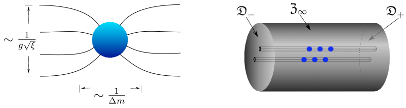
Figure 1: The left figure shows a confined monopole in close up with the characteristic scales for the monopole size displaying approximate Coulomb monopole behavior and the size of the confining vortex. The right figure depicts the spatial boundary, a cylinder at infinity, where the asymptotic behavior of the (multiple) confined monopoles is specified (see main text). The cylinder at infinity consists of the two discs $\mathfrak{D}_{\pm}$ at $x^{3}\rightarrow\pm\infty$ and the cylinder wall $\mathfrak{Z}_{\infty}$ at $r\rightarrow\infty$, with $r$ being the cylindrical radial coordinate.

The paper is organized as follows: In section 2. we describe three different formulations of the model to discuss different properties. In particular we introduce an embedding in a six-dimensional theory which is crucial for the quantum computations. In section 3. we discuss the super-multiplet structure of confined monopoles. To do so we identify tensorial central charges in the susy algebra. In addition we discuss the $SU(2)_{R}$ action on the associated BPS equations. In section 4. we perform the quantization of the confined monopoles and compute the quantum energies for these objects, identify an anomaly in the central charge and compare our results with the BPS spectrum of $CP^{n}$ models. In section 5. we summarize our results and present conclusions.

2 Three Faces of ${\cal N}=2$ SQCD

In this section we give three different formulations of ${\cal N}=2$ SQCD with $N_{f}$ massive quark multiplets and a generalized Fayet-Iliopoulos FI-term. Each of the three formulations will allow us to analyze different aspects in a useful way. First we introduce a ${\mathcal{N}}=1$ superspace formulation to list some basic properties of the model and in particular discuss the vacua and symmetry breaking patterns in a conventional way. Secondly we give an $SU(2)_{R}$ covariant component formulation which will set the conventions for the subsequent sections and notably be the starting point for a six-dimensional formulation of the theory. Lastly we construct a six-dimensional model in which the four-dimensional theory can be embedded. This formulation is of utmost importance for the consistently regularized quantization procedure in the presence of monopoles and vortices. The gauge group is chosen to be $U(N)$ and in general we assume that $N_{f}\geq N$, as discussed in the introduction.

2.1 ${\cal N}=1$ Superspace and Vacuum Moduli

The ${\cal N}=2$ SQCD Lagrangian is given by the coupling of a ${\cal N}=2$ vector multiplet in the adjoint representation to $N_{f}$ hypermultiplets in the fundamental representation of the gauge group. In ${\cal N}=1$ superspace the ${\cal N}=2$ vector multiplet is composed of a vector multiplet $V\sim(A_{\mu},\lambda,D)$ and a chiral multiplet $\Phi\sim(\phi,\psi,F)$, both in the adjoint representation. The $i=1,\ldots,N_{f}$ hypermultiplets are composed of two sets of chiral multiplets $Q_{i}\sim(q_{i},\chi_{i},F_{i})$ and $\tilde{Q}_{i}\sim(\tilde{q}_{i},\tilde{\chi}_{i},\tilde{F}_{i})$, where $Q_{i}$ transforms in the fundamental ${\bf N}$ of $U(N)$, whereas $\tilde{Q}_{i}$ transforms in the conjugate representation ${\bf\bar{N}}$. Similarly, w.r.t. the flavor group $SU(N_{f})$ the multiplets $Q_{i},\tilde{Q}_{i}$ are in the representation ${\bf N_{f}}$ and ${\bf\bar{N}_{f}}$, respectively, though we do not indicate this by the index position. We do not include a vacuum theta-angle. The superspace Lagrangian is given by

$${\mathcal{L}}= \ \ \mathrm{Tr}\ \big{\{}\,\tfrac{2}{g^{2}}\int d^{2}\theta\,W^{\alpha}W_{\alpha}+h.\,c.+\tfrac{2}{g^{2}}\int d^{4}\theta\,e^{2V}\Phi^{\dagger}e^{-2V}\Phi$$

$$\hskip 113.81102pt+2\,\xi_{3}\int d^{4}\theta\,V-{\textstyle{\frac{i}{\sqrt{2}}}}\,\bar{\xi}\int d^{2}\theta\,\Phi+h.\,c.\big{\}}$$

$$+\int d^{4}\theta\,(\,\bar{Q}_{i}\,e^{-2V}Q_{i}+\tilde{Q}_{i}\,e^{2V}\bar{\tilde{Q}}_{i}\,)+\sqrt{2}\int d^{2}\theta\,(\,\tilde{Q}_{i}\Phi\,Q_{i}+m_{i}\tilde{Q}_{i}Q_{i}+h.\,c.).$$ (1)

The first line describes pure ${\cal N}=2$ SYM and the second line resembles a generalized FI-term and is non-vanishing for $U(N)$ or any $U(1)$ factor in the considered gauge group. The first FI-term is a standard FI-$D$-term whereas the second term, the non-standard FI-$F$-term, can be obtained from a soft breaking mass term for the adjoint chiral field $\Phi$ which to first order preserves ${\cal N}=2$ supersymmetry [8, 22]. See also the comments in the introduction. The FI-parameters $\xi_{3}$ and $\xi=\xi_{1}+i\xi_{2}$ form an $SU(2)_{R}$ vector (triplet) $\vec{\xi}$ [19] which explicitly breaks the $SU(2)_{R}$ symmetry. At the considered scale within the mentioned approximation this allows one to interpret all FI-terms to be of dynamical origin due to a soft breaking term. Different choices for $\vec{\xi}$, including the standard FI-$D$-term which is usually put in by hand, are related to each other by $SU(2)_{R}$ transformations. We will make use of this in more detail below. This is similar to the explicit breaking of the flavor symmetry $SU(N_{f})$ by the masses $m_{i}$ which was used to bring the mass matrix into diagonal form (for ${\mathcal{N}}=2$ supersymmetry the mass matrix has to commute with its hermitian conjugate [9]).

The last line is the Lagrangian for the quark multiplets, which turns pure SYM into SQCD. The superpotential contains a priori complex masses $m_{i}$ whose specific values are crucial for the resulting dynamics. Eventually we will choose them to be real and they can be ordered by $SU(N_{f})$ Weyl reflection such that $m_{1}\leq m_{2}\leq\ldots\leq m_{N_{f}}$. Their relative values determine the symmetry breaking pattern of the gauge group as well as the explicit breaking of the $SU(N_{f})$ flavor symmetry. For generic masses $U(N)$, $SU(N_{f})$ is broken to $U(1)^{N}$, $U(1)^{N_{f}-1}$ at the scale of the bare masses $m_{i}$, which are defined at a UV cut-off scale $M_{UV}$. The coefficient for the superpotential is chosen such that the theory has ${\cal N}=2$ supersymmetry, there is no independent coupling for it.

For the generators of the gauge group $U(N)$ we have the following conventions: The hermitian generators are $\{T^{A}\}=\{T^{0},T^{a}\}$, where $\{T^{a}\}$ forms an $su(N)$ algebra, and satisfy

$$[T^{a},T^{b}]=if^{abc}\,T^{c}\ ,\ \ T^{0}={\textstyle{\frac{1}{\sqrt{2N}}}}\mathds{1}\ ,\ \ \mathrm{Tr}\{T^{A}T^{B}\}={\textstyle{\frac{1}{2}}}\,\delta^{AB}\ ,$$ (2)

where $f^{abc}$ are the real and totally antisymmetric $su(N)$ structure constants.

Classical Vacua. The Lagrangian (2.1), though only explicitly realizing ${\mathcal{N}}=1$ supersymmetry, is a convenient way to discuss the vacuum moduli. The presence of the FI-terms drives the the theory into the Higgs phase at the scale where they become relevant. The different possible vacua lead to different symmetry breaking patterns and associated topological field configurations. We discuss this in the following.

The bosonic potential of (2.1) can be written in terms of the on-shell component auxiliary fields $D$, $F$ and $F_{i}$, $\tilde{F}_{i}$,

$$-{\mathcal{L}}_{\mathrm{aux}}=V_{\mathrm{bos}}={\textstyle{\frac{2}{g^{2}}}}\,\mathrm{Tr}\,\{{\textstyle{\frac{1}{2}}}\,D^{2}+FF^{\dagger}\}+\sum_{i}\,|F_{i}|^{2}+|\tilde{F}_{i}|^{2}\,,$$ (3)

where the auxiliary fields are given by

$$D=[\phi,\phi^{\dagger}]+{\textstyle{\frac{g^{2}}{2}}}(q_{i}\otimes\bar{q}_{i}-\bar{\tilde{q}}_{i}\otimes\tilde{q}_{i}-\xi_{3}\mathds{1})\ ,\ \ F^{\dagger}=-{\textstyle{\frac{g^{2}}{\sqrt{2}}}}\,(q_{i}\otimes\tilde{q}_{i}-{\textstyle{\frac{i}{2}}}\,\bar{\xi}\,\mathds{1})$$

$$\hskip 42.67912ptF_{i}=-\sqrt{2}(\phi^{\dagger}+\bar{m}_{i})\bar{\tilde{q}}_{i}\ ,\ \ \bar{\tilde{F}}_{i}=-\sqrt{2}(\phi+m_{i})q_{i}\ ,$$ (4)

and there is no summation over flavor indices in the second line. Generally we employ a matrix notation for the adjoint fields, accordingly the tensor product in the first line is defined w.r.t. gauge indices. The vanishing of the potential (3) thus implies the conditions

$$[\phi,\phi^{\dagger}]=0\,,$$

$$q_{i}\otimes\tilde{q}_{i}={\textstyle{\frac{i}{2}}}\,\bar{\xi}\,\mathds{1}\ \ ,\ \ q_{i}\otimes\bar{q}_{i}-\bar{\tilde{q}}_{i}\otimes\tilde{q}_{i}=\xi_{3}\mathds{1}\,,$$

$$(\phi+m_{i})q_{i}=0\ ,\ \ (\phi^{\dagger}+\bar{m}_{i})\bar{\tilde{q}}_{i}=0\ ,$$ (5)

which are of the same form as for $SU(N)$ theory [9] except for the absence of the condition $\mathrm{Tr}\,\phi=0$ and that the FI-parameters $\vec{\xi}$ fix the moduli of the Higgs branch equations. We refer to [9] for further details, but here we are interested in a certain set of vacua for which the squark fields $q_{i}$, $\tilde{q}_{i}$, written as $N\times N_{f}$ matrices, take the form

$$[q^{\mathrm{vac}}]^{n}{}_{i}=\begin{bmatrix}\kappa_{1}&&&0&&&0&\\ &\ddots&&&\ddots&&&\ddots\\ &&\kappa_{N}&&&0&&\end{bmatrix}\ ,\ \ [\tilde{q}^{\mathrm{vac}}]_{ni}=\begin{bmatrix}\tilde{\kappa}_{1}&&&0&&&0&\\ &\ddots&&&\ddots&&&\ddots\\ &&\tilde{\kappa}_{N}&&&0&&\end{bmatrix}\ ,$$ (6)

where we assumed for the moment that $N_{f}\geq 2N$ and indicated that these are the vacuum values of the fields. In general we will assume only $N_{f}\geq N$, which is taken into account by erasing the appropriate number of columns in (6). The Higgs branch equations, the second line in (2.1), give

$$|\kappa_{n}|^{2}-|\tilde{\kappa}_{n}|^{2}=\xi_{3}\ \ \ \textrm{and}\ \ \ \kappa_{n}\tilde{\kappa}_{n}={\textstyle{\frac{i}{2}}}\,\bar{\xi}\ ,\ \ \forall\,n=1,\ldots,N\ .$$ (7)

For certain solutions of (7) the vacuum preserves the symmetry $SU(N)_{C+F}=\mathrm{diag}(U(N)_{C}\times SU(N)_{F})$. This symmetry of the so called color-flavor locked phase is the key aspect for the existence of non-abelian vortices [12]. We therefore set $\kappa_{n}=\kappa$ and $\tilde{\kappa}_{n}=\tilde{\kappa}$ for all $n$. Inserting in (6) and deleting the trivial columns shows that

$$U_{C}\,q^{\mathrm{vac}}\,U_{F}=q^{\mathrm{vac}}\ \ ,\ \ U^{\dagger}_{F}\,\tilde{q}^{\mathrm{vac}}\,U^{\dagger}_{C}=\tilde{q}^{\mathrm{vac}}\ ,$$ (8)

where $U_{C}\in U(N)$, $U_{F}\in SU(N_{f})$ are $SU(N)$ transformations with $U_{C}=U_{F}^{-1}=:U_{C+F}$.

The actual values of $\kappa$, $\tilde{\kappa}$ depend on the FI-parameters and are determined by (7). There are two special choices which appear in the literature. i.) $\xi=0$, $\xi_{3}>0$ gives $\tilde{q_{i}}^{\mathrm{vac}}=0$, and $q^{\mathrm{vac}\,n}_{i}=\sqrt{\xi_{3}}\,\delta^{n}_{i}$. ii.) $\xi_{3}=0$, $\xi_{1}=0$, $\xi_{2}>0$ gives $\tilde{q}^{\mathrm{vac}}_{ni}=q^{\mathrm{vac}\,n}_{i}=\sqrt{\xi_{2}/2}\,\delta^{n}_{i}$. The phases of $q_{i}^{\mathrm{vac}}$, $\tilde{q_{i}}^{\mathrm{vac}}$ have been fixed by gauge symmetry. A nontrivial winding in these phases describes topologically stabilized configurations. The classification of such states is given by the symmetry breaking pattern of the vacuum,

$$U(N)\times SU(N_{f})\overset{\sqrt{\xi}}{\longrightarrow}SU_{C+F}(N)\,,$$ (9)

where the breaking of the overall $U(1)\subset U(N)$ guarantees vortex solutions which are topologically stabilized according to $\pi_{1}(U(1))=\mathbb{Z}$ and are non-abelian for $N>1$ due to the preserved color-flavor symmetry $SU_{C+F}(N)$.

This is of course not the whole story since a vev for the adjoint scalar may break the gauge group to a subgroup of $U(N)$ already at a higher scale, as we will assume in the following. For non-vanishing FI-parameters either $\kappa$ or $\tilde{\kappa}$ is non-vanishing and thus the last two conditions in (2.1) imply for the vev $\phi_{0}$ of $\phi$,

$$\phi_{0}=-\begin{bmatrix}m_{1}&&\\ &\ddots&\\ &&m_{N}\end{bmatrix}\ ,\quad\quad\textrm{with}\quad H_{C}\,\phi_{0}\,H^{-1}_{C}=\phi_{0}\ ,$$ (10)

which thus automatically satisfies the first condition in (2.1). For generic masses the gauge symmetry is completely broken ($SU(N_{f})$ is explicitly broken). However, if some masses coincide the unbroken subgroup $H_{C}\subset U(N)$ is non-abelian and also the flavor group $SU(N_{f})$ is not completely broken and hence part of the color-flavor symmetry (8) remains intact. Consequently, the symmetry breaking pattern is given by

$$U(N)\times SU(N_{f})\overset{m}{\longrightarrow}U_{C}(1)\times H_{C}\times H_{F}\overset{\sqrt{\xi}}{\longrightarrow}H_{C+F}\,,$$ (11)

where we assumed that all masses are of the same scale and that $m\gg\sqrt{\xi}$. If the first $N$ masses form $q$ groups of $n_{r}$ degenerate masses the surviving symmetry group is given by [23]

$$H_{C+F}=S(\,U(n_{1})\times\ldots\times U(n_{q})\,)\,,$$ (12)

with $\sum_{r}n_{r}=N$. It supports monopoles with typical size $1/\Delta m$, the inverse mass difference, and are confined by flux tubes of width $\sim 1/g\sqrt{\xi}$, see figure 1.

2.2 $SU(2)_{R}$ Covariant Formulation

The component form of the Lagrangian (2.1) can be easily obtained by using the formulas given in [21]. Here we give the resulting component Lagrangian directly in the $SU(2)_{R}$ covariant form. For this one groups the adjoint fermions of the ${\mathcal{N}}=2$ vector multiplet $(V,\Phi)$ and the fundamental scalars of the quark multiplets $(Q_{i},\bar{\tilde{Q}}_{i})$ into $SU(2)_{R}$ doublets $\lambda_{\alpha I}$ and $S_{iI}$, respectively:

$$\lambda_{\alpha I}:=(\lambda_{\alpha},\psi_{\alpha})\ \ ,\ \ S_{iI}:=(q_{i},i\bar{\tilde{q}}_{i})\ ,$$ (13)

with $(\lambda_{\alpha I})^{\dagger}=:\bar{\lambda}^{I}_{\dot{\alpha}}$ and $(S_{iI})^{*}=:\bar{S}^{I}_{i}$. With this notation the resulting component Lagrangian obtained from (2.1) can be written in the following form:

$${\mathcal{L}}_{4D} =$$

$${\textstyle{\frac{2}{g^{2}}}}\,\mathrm{Tr}\,\{-{\textstyle{\frac{1}{4}}}F_{\mu\nu}^{2}-|D_{\mu}\phi|^{2}-i\bar{\lambda}^{I}\bar{\not{D}}\lambda_{I}\}-|D_{\mu}S_{iI}|^{2}-i(\bar{\chi}_{i}\bar{\not{D}}\chi_{i}+\bar{\tilde{\chi}}_{i}\bar{\not{D}}\tilde{\chi}_{i})$$

$$-{\textstyle{\sqrt{2}}}\,\big{[}\,{\textstyle{\frac{i}{g^{2}}}}\,\mathrm{Tr}\,\{\varepsilon_{IJ}\,\bar{\lambda}^{I}[\,\bar{\lambda}^{J},\phi]\}+i\bar{S}^{I}_{i}(\lambda_{I}\chi_{i}-i\,\varepsilon_{IJ}\bar{\lambda}^{J}\bar{\tilde{\chi}}_{i})+\tilde{\chi}_{i}(\phi+m_{i})\chi_{i}+h.c.\big{]}$$

$$-{\textstyle{\frac{2}{g^{2}}}}\,\mathrm{Tr}\,\{\,{\textstyle{\frac{1}{2}}}[\phi,\phi^{\dagger}]{}^{2}-{\textstyle{\frac{1}{2}}}\,{\vec{{\mathsf{D}}}}^{2}+{\textstyle{\frac{1}{2}}}\,g^{2}\,\vec{{\mathsf{D}}}\cdot(\vec{\tau}_{I}{}^{J}S_{i\,J}\otimes\bar{S}^{I}_{i}-\vec{\xi}\ \mathds{1})\}$$

$$\hskip 213.39566pt-\bar{S}^{I}_{i}\{\phi^{\dagger}+\bar{m}_{i},\phi+m_{i}\}S_{i\,I}\ ,$$ (14)

where the first line contains the kinetic terms with $\bar{\not{D}}=\bar{\sigma}^{\mu}D_{\mu}$, and the second line gives the Yukawa couplings. The $SU(2)_{R}$ $\varepsilon$-tensor is defined as $\varepsilon^{12}=\varepsilon_{12}=1$ and we use the convention $(\varepsilon_{IJ})^{*}=(\varepsilon^{IJ})$. The residual terms are the bosonic potential terms where the braces in the last term denotes the anti-commutator of the given matrices.

Here we introduced an $SU(2)_{R}$ triplet of auxiliary fields $\vec{{\mathsf{D}}}$ and the $SU(2)_{R}$ Pauli matrices $\vec{\tau}$. The introduction of these auxiliary fields does not result in an off-shell closure of the supersymmetry algebra [24] but considerably simplifies many manipulations. On-shell the auxiliary triplet is given by

$$\vec{{\mathsf{D}}}=\frac{g^{2}}{2}\,(\vec{\tau}_{I}{}^{J}S_{i\,J}\otimes\bar{S}^{I}_{i}-\vec{\xi}\ \mathds{1})\ .$$ (15)

This form of the Lagrangian is, up to the FI-vector $\vec{\xi}$, manifestly invariant under the $SU(2)_{R}$ symmetry which acts on the adjoint fermion doublet $\lambda_{\alpha I}$ and the squark scalar doublet $S_{iI}$ (and of course the auxiliary triplet $\vec{{\mathsf{D}}}$). All other fields are singlets under $SU(2)_{R}$.

It has turned out that the embedding of a theory with solitons into higher dimensions is a crucial step in computing quantum corrections for (topologically) nontrivial states in a tractable and consistent way [25, 26]. In the next step we will embed ${\mathcal{N}}=2$ SQCD with masses and FI-terms in six-dimensional space. This embedding and the relation to four-dimensional physics is most conveniently found starting from the four-dimensional Lagrangian in the form (2.2).

2.3 Six-Dimensional Embedding

As is well known, pure ${\mathcal{N}}=2$ SYM in four dimensions can be obtained by dimensional reduction from pure ${\mathcal{N}}=1$ SYM in six dimensions [27]. In extending this method to ${\mathcal{N}}=2$ SQCD one has to handle the masses and the extra field content from the quark hypermultiplet.

We first introduce the conventions for six-dimensional fermions, where we follow closely [28]. We label coordinates by $x^{M}$, $M=0,1,2,3,5,6$, where $x^{5}$, $x^{6}$ are the extra dimensions compared to the four-dimensional world. The six-dimensional gamma matrices $\Gamma^{M}$ and the chirality and charge conjugation matrices $\Gamma_{7}$, $C$ we define as

$$\Gamma_{7}:=\Gamma_{0}\Gamma_{1}\Gamma_{2}\Gamma_{3}\Gamma_{5}\Gamma_{6}\ ,\ \ \Gamma_{7}{}^{2}=\mathds{1}\ ,\ \ \Gamma_{7}{}^{\dagger}=\Gamma_{7}\ ,\ \ C\,\Gamma^{M}C^{-1}=-{\Gamma^{M}}^{T}.$$ (16)

For the fermions we introduce symplectic Majorana-Weyl spinors $\lambda_{I=1,2}$, which are in the adjoint of the gauge group, and $N_{f}$ anti-chiral spinors $\psi_{i=1\ldots N_{f}}$ which are in the fundamental representation. These are eight-component spinors in six dimensions and satisfy

$$\Gamma_{7}\,\psi_{i}=-\psi_{i}\ \ ,\ \ \Gamma_{7}\,\lambda_{I}=\lambda_{I}\ \ ,\ \ \lambda_{I}=\varepsilon_{IJ}\,C^{-1}\,{\bar{\lambda}}^{J^{T}}\ .$$ (17)

Here the bar stands for Dirac conjugation, ${\bar{\lambda}}^{J}=(\lambda_{J})^{\dagger}\,i\Gamma^{0}$, and the symplectic Majorana-Weyl condition can be equivalently written as ${\bar{\lambda}}^{I}=-\varepsilon^{IJ}\lambda_{J}^{T}C$.

Next we introduce a $U(N)$ gauge field $A_{M}$ in six dimensions whose extra components give the adjoint scalars upon dimensional reduction. To also generate the masses for the (anti) fundamental matter fields in (2.2) we introduce additional constant $U(1)$ background gauge fields in the extra dimensions, $\hat{A}_{5}$ and $\hat{A}_{6}$, so that $A_{M}=(A_{\mu},\,A_{5}+\hat{A}_{5},\,A_{6}+\hat{A}_{6})$. The $i$’th flavor couples to these $U(1)$ backgrounds with charges $e_{5\,i}$, $e_{6\,i}$ if it is in the fundamental representation and with the negative thereof if it is in the anti-fundamental representation of the gauge group. Hence one has for example

$$D_{5/6}\psi_{i}=\partial_{5/6}\psi_{i}-i(A_{5/6}+e_{5\,i/6\,i})\psi_{i}\ .$$ (18)

We introduce the same set of scalars $S_{iI}$ and their conjugates in six dimensions as in (2.2), which also couple to the constant $U(1)$ backgrounds $\hat{A}_{5}$, $\hat{A}_{6}$ in the described manner, i.e. analogous to (18). As in four dimensions we define the covariant derivatives of the adjoint fields and the six-dimensional field strength as

$$F_{MN} =\partial_{M}A_{N}-\partial_{N}A_{M}-i[A_{M},A_{N}]\ ,$$

$$D_{M}\lambda_{I} =\partial_{M}\lambda_{I}-i[A_{M},\lambda_{I}]\ .$$ (19)

Clearly, the constant $U(1)$ backgrounds enter exclusively through the coupling (18).

The six-dimensional ${\mathcal{N}}=1$ SQCD Lagrangian with FI-term is

$${\mathcal{L}}_{6D}={\textstyle{\frac{2}{g^{2}}}}\,\mathrm{Tr}\,\{ -{\textstyle{\frac{1}{4}}}F_{MN}^{\,2}-{\textstyle{\frac{1}{2}}}\bar{\lambda}^{I}\not{D}\lambda_{I}+{\textstyle{\frac{1}{2}}}\,{\vec{{\mathsf{D}}}}^{2}-{\textstyle{\frac{1}{2}}}\,g^{2}\,\vec{{\mathsf{D}}}\cdot(\vec{\tau}_{I}{}^{J}S_{i\,J}\otimes\bar{S}^{I}_{i}-\vec{\xi}\ \mathds{1})\}$$

$$-|D_{M}S_{iI}|^{2}-\bar{\psi}_{i}\not{D}\,\psi_{i}+i\sqrt{2}\,(\,\varepsilon_{IJ}\,\bar{S}^{I}_{i}\,\bar{\lambda}^{J}\psi_{i}+\varepsilon^{IJ}\,\bar{\psi}_{i}\,\lambda_{I}S_{iJ})\ ,$$ (20)

where $\not{D}=\Gamma^{M}D_{M}$, keeping in mind the additional $U(1)$ backgrounds. The six-dimensional Lagrangian (2.3) is constructed in such a way that upon trivial dimensional reduction, i.e. by taking all fields independent of $x^{5}$ and $x^{6}$, one obtains the four-dimensional Lagrangian (2.2).

Dimensional Reduction. The first step is to choose a representation for the six-dimensional gamma matrices $\Gamma^{M}$ in terms of four-dimensional gamma matrices $\gamma^{\mu}$ and decompose the spinors accordingly. Following [28] we choose

$$\Gamma^{\mu} =\gamma^{\mu}\otimes\sigma^{1}\ ,\ \ \Gamma_{5}=\gamma_{5}\otimes\sigma^{1}\ ,\ \ \Gamma_{6}=\mathds{1}\otimes\sigma^{2}\ ,$$

$$C =C_{4D}\,\gamma_{5}\otimes\sigma^{2}\ ,\ \ \Gamma_{7}=\mathds{1}\otimes\sigma^{3}\ ,$$ (21)

where the form of $\Gamma_{7}$ follows from its definition in (16) which also implies that $\gamma_{5}=i\gamma_{0}\gamma_{1}\gamma_{2}\gamma_{3}$. The chirality conditions (17) thus imply that the six-dimensional eight component spinors are decomposed into four-dimensional four-component spinors as

$$\lambda^{6D}_{I}=\lambda^{4D}_{I}\otimes\textstyle{\binom{1}{0}}\ \ ,\ \ \psi^{\,6D}_{i}=\psi_{i}^{\,4D}\otimes\textstyle{\binom{0}{1}}\ ,$$ (22)

where in the following we will omit the indication of the dimension; it will be clear from the context. To make contact with our four-dimensional ${\mathcal{N}}=2$ SQCD Lagrangian (2.2) we choose a chiral representation for the four-dimensional gamma matrices $\gamma^{\mu}$ and decompose the four-component spinors into Weyl spinors as follows:

$$\gamma^{\mu}=i\begin{pmatrix}0&\sigma^{\mu}\\ \bar{\sigma}^{\mu}&0\end{pmatrix}\ \ ,\ \ \lambda_{I}=\begin{bmatrix}-i\,\lambda_{\alpha I}\\ \varepsilon_{IJ}\bar{\lambda}^{\dot{\alpha}\,J}\end{bmatrix}\ \ ,\ \ \psi_{i}=\begin{bmatrix}\,\chi_{\alpha i}\,\\ \,\bar{\tilde{\chi}}_{i}^{\dot{\alpha}}\,\end{bmatrix}\ ,$$ (23)

and the charge conjugation matrix is given by $C_{4D}=i\,\gamma^{2}\gamma^{0}$. Inserting these decompositions into the six-dimensional Lagrangian (2.3) and taking all fields independent of the extra coordinates $x^{5,6}$ one finds the original four-dimensional Lagrangian (2.2) upon the following identifications:

$$\phi=\frac{1}{\sqrt{2}}\,(i\,A_{5}-A_{6})\ \ ,\ \ m_{i}=\frac{1}{\sqrt{2}}\,(i\,e_{5\,i}-e_{6\,i})\ .$$ (24)

The mechanism introduced here for generating the masses in the lower dimensional theory is rather different from the usual Scherk-Schwarz mechanism [29]. It is similar to the method used in gauged $CP^{n}$ sigma models to generate twisted mass terms via constant background gauge fields [30]. Nevertheless it would be interesting to have a brane interpretation of this mechanism.

To obtain the four-dimensional Lagrangian (2.2) we consequently had to choose a chiral representation for the four-dimensional gamma matrices. However, for determining quantum corrections for confined monopoles we will have to use a different representation to make use of the flat extra dimensions as a regulator. This will be discussed in more detail below.

3 Tensorial Central Charges and $\frac{1}{4}$ BPS Equations

In this section we analyze the supersymmetry structure of ${\mathcal{N}}=2$ SQCD, especially the influence of the FI-terms. In particular we will find tensorial central charges in the local superalgebra (or in the global algebra in compact space). Usually such charges are not considered in the ${\mathcal{N}}=2$ susy algebra, though they are common for example in the M-theory superalgebra [31], but they are essential for the objects under investigation (see however recent developments in the context of six-dimensional $(2,0)$ theories compactified to four dimensions [32] and considerations for ${\mathcal{N}}=1$ theories [33, 34]). These tensorial central charges are carried by extended objects such as the vortices which confine the monopoles or domain walls. The relation of these structures to the $\frac{1}{4}$ BPS equations, which also describe confined monopoles, will be described in the following.

3.1 Supercurrent and SUSY Algebra

It will be most convenient to start in the six-dimensional setting (2.3). The Lagrangian (2.3) is invariant up to total derivative terms under the following susy transformations

$$\delta\vec{{\mathsf{D}}} =-i\,\bar{\eta}^{I}\vec{\tau}_{I}{}^{J}\,\not{D}\,\lambda_{J}\hskip 99.58464pt\delta S_{iI}=-\sqrt{2}\,\varepsilon_{IJ}\,\bar{\eta}^{J}\,\psi_{i}$$

$$\delta A_{M} =\,\bar{\eta}^{I}\Gamma_{M}\lambda_{I}\hskip 130.88284pt\delta\psi_{i}=-\sqrt{2}\,\varepsilon^{IJ}\not{D}S_{Ii}\eta_{J}$$

$$\delta\lambda_{I} =-{\textstyle{\frac{1}{2}}}\,F_{MN}\Gamma^{MN}\,\eta_{I}+i\,\vec{{\mathsf{D}}}\cdot\vec{\tau}_{I}{}^{J}\eta_{J}\ ,$$ (25)

where in the left column are the standard transformations of the gauge multiplet supplemented by the transformation of the adjoint auxiliary triplet and on the right are the transformations of the matter multiplet. Obviously the six-dimensional language and the use of the auxiliary field crucially simplifies the structure. The transformation parameter $\eta_{I}$ is (like $\lambda_{I}$) a chiral symplectic Majorana-Weyl spinor and satisfies the relations given in (17).

To determine the associated supercurrent one can use different versions of the Noether theorem, for example transforming the Lagrangian with local susy parameters. However, every procedure has some ambiguity in the resulting current. See for example [28] and the relevance of improvement terms in this context. We determine here the supercurrent in the following way: i.) Given that the current is fermionic and linear in the fermionic fields we make the most general ansatz linear in $\lambda_{I}$ and $\psi_{i}$ and their conjugates. ii.) Since the parameter $\eta_{I}$ of the susy transformations (3.1) is a chiral symplectic Majorana-Weyl spinor the associated supercurrent $J^{M}_{I}$ has to be an anti-chiral symplectic Majorana-Weyl spinor and thus satisfies

$$\Gamma_{7}\,J^{M}_{I}=-J^{M}_{I}\ \ ,\ \ J^{M}_{I}=\varepsilon_{IJ}\,C^{-1}\bar{J}^{M\,J^{\,T}}\ .$$ (26)

Consequently the susy transformation of fields is generated by the commutator

$$\delta^{\mathrm{susy}}=i\ [\,\int_{\vec{x}}\bar{\eta}^{I}J^{0}_{I}\,,\ \ ]=i\ [\,\bar{\eta}^{I}Q_{I}\,,\ \ ]\ .$$ (27)

Given these preliminaries we determine the susy current and fix its ambiguities by the requirement that the transformation (27) generates the susy transformations of the fermions in (3.1) without surface terms, through the canonical anti-commutators derived from the Dirac brackets. This requirement and Lorentz covariance gives a unique current in accordance with the transformations of the elementary fields (3.1):

$$J^{M}_{I}=\, {\textstyle{\frac{2}{g^{2}}}}\mathrm{Tr}\,\{{\textstyle{\frac{1}{2}}}\,F_{PQ}\,\Gamma^{PQ}\Gamma^{M}\lambda_{I}-i\,\vec{{\mathsf{D}}}\cdot\vec{\tau}_{I}{}^{J}\Gamma^{M}\lambda_{J}\,\}$$

$$\ \ +{\textstyle{\sqrt{2}}}\ \Gamma^{N}\Gamma^{M}(\,C^{-1}\bar{\psi}_{i}^{T}D_{N}S_{iI}-\varepsilon_{IJ}D_{N}\bar{S}^{J}_{i}\psi_{i}\,)\ .$$ (28)

It is easy to check that this current is conserved on-shell.

Supersymmetry Algebra. The variation of the supercurrent under the susy transformations (3.1) gives the local susy algebra. Using the fermionic e.o.m. and the on-shell condition (15) for the auxiliary triplet the resulting transformation of the current (3.1) can be written in the form

$$\delta\,J^{M}_{I}=-2\,[\,\delta_{I}{}^{J}\,(\,T^{MN}-{\textstyle{\frac{1}{4}}}\,\varepsilon^{MNPQRS}{\mathcal{Z}}_{PQRS}\,)\,\Gamma_{N}+{\mathcal{Z}}_{I}{}^{J}{}_{PQ}\,\Gamma^{MPQ}\,]\,\eta_{J}\ ,$$ (29)

where we did not write a fermionic topological term. The first contribution in (29) is the on-shell gravitational stress tensor

$$T^{MN}= \ {\textstyle{\frac{2}{g^{2}}}}\mathrm{Tr}\,\{F^{MP}F^{N}{}_{P}\}\,+\,2\,D^{(M}\bar{S}^{K}_{i}D^{N)}S_{iK}$$

$$+\,{\textstyle{\frac{1}{g^{2}}}}\mathrm{Tr}\,\{\bar{\lambda}^{K}\Gamma^{(M}D^{N)}\lambda_{K}\}+{\textstyle{\frac{1}{2}}}\,\bar{\psi}_{i}\,\Gamma^{(M}\overset{\leftrightarrow}{D}{}^{N)}\psi_{i}+\eta^{MN}{\mathcal{L}}_{6D}\ ,$$ (30)

where the $\lambda$-term is hermitian due to the symplectic Majorana-Weyl condition and the fermionic part in ${\mathcal{L}}_{6D}$ vanishes on-shell.

The local topological charges, or charge densities, are given by

$${\mathcal{Z}}_{PQRS}= \ {\textstyle{\frac{1}{g^{2}}}}\mathrm{Tr}\,\{F_{[PQ}F_{RS]}\}+{\textstyle{\frac{1}{6}}}\,\partial_{[P}\,\big{(}\,{\textstyle{\frac{1}{g^{2}}}}\mathrm{Tr}\,\{\bar{\lambda}^{K}\Gamma_{QRS]}\lambda_{K}\}-\bar{\psi}_{i}\Gamma_{QRS]}\psi_{i}\,\big{)}\ ,$$

$${\mathcal{Z}}_{I}{}^{J}{}_{PQ}= \ \vec{\tau}_{I}{}^{J}\cdot[\,{\textstyle{\frac{i}{2}}}\,\vec{\xi}\ \mathrm{Tr}\,F_{PQ}+\partial_{[P}(\bar{S}_{i}\,\vec{\tau}\,D_{Q]}S_{i})\,]$$ (31)

The first charge corresponds to the standard central charge of the ${\mathcal{N}}=2$ susy algebra in four dimensions. The fermionic terms are of the form discussed in footnote 10 and they are not relevant for the following discussion, see however related comments in the next section. In four dimensions the four-form corresponds to a point like object (by duality) just like the usual (un-confined) monopole in the Coulomb phase. The second charge, however, is a two-form and thus corresponds to an extended object also in four dimensions. Depending on the location in six-dimensional space these charges may describe two-branes (domain walls) or one-branes (strings) in four dimensions. Clearly the presence of such charges breaks four-dimensional Lorentz symmetry and they are therefore usually not considered in the general structure of ${\mathcal{N}}=2$ susy-algebra. Equivalently one can show that these charges cannot be carried by finite energy states in $\mathbb{R}^{3+1}$. Putting the system in a compact spatial volume circumvents this problem. For the moment we continue considering the local susy algebra and by dimensional reduction we will see the explicit realization of the above statements.

Dimensional Reduction. Inserting the dimensional reduction rules (2.3) - (24) into the zero component of (29), one obtains according to equation (27) the four-dimensional local susy algebra in the following form:

$$\{Q_{\alpha I},j^{0}_{\,\beta J}\}= \ 2\,\sqrt{2}\,[\ \varepsilon_{IJ}\,\varepsilon_{\alpha\beta}\,{\mathcal{Z}}-(\vec{\tau}\varepsilon)_{IJ}\cdot\vec{{\mathcal{T}}}^{\mathrm{w}}_{k}\,(\sigma^{k}\varepsilon)_{\alpha\beta}\ ]\ ,$$

$$\{\bar{Q}_{\dot{\beta}}{}^{J}\,,j^{0}_{\,\alpha I}\}= \ 2\,[\,\delta_{I}{}^{J}\,{\mathscr{P}}_{\mu}\,\sigma^{\mu}_{\alpha\dot{\beta}}+\vec{\tau}_{I}{}^{J}\cdot\vec{{\mathcal{T}}}^{\mathrm{v}}_{k}\,\sigma^{k}_{\alpha\dot{\beta}}\,]\ ,$$ (32)

where the index $k=1,2,3$ runs only over the spatial components, a convention we will in general use for small Latin indices, and $\sigma^{k}$ are thus the Pauli matrices. Note that the matrices $(\vec{\tau}\varepsilon)_{IJ}$ and equivalently $(\sigma^{k}\varepsilon)_{\alpha\beta}$ are symmetric.

The objects on the r.h.s. are the following: $\mathscr{P}_{\mu}$ is the four-dimensional momentum density $T^{0}{}_{\mu}$ and the charge density ${\mathcal{Z}}$ is the usual central charge contribution,

$${\mathcal{Z}}={\textstyle{\frac{2}{g^{2}}}}\,\partial_{k}\mathrm{Tr}\,\{\phi^{\dagger}(B_{k}+iE_{k})\}\,,$$ (33)

which is carried by point-like objects such as un-confined monopoles or dyons. The electric and magnetic field contributions stem from $T^{0}{}_{5/6}$ and ${\mathcal{Z}}_{i\,j\,k\,5/6}$ in the six-dimensional theory and are thus both carried by pointlike objects in three spatial dimensions. The actual electric and magnetic charge of such objects is proportional to the imaginary and real part of ${\mathcal{Z}}$, respectively.

The less standard terms in (3.1) are the $SU(2)_{R}$ vector charge densities

$$\vec{{\mathcal{T}}}^{\mathrm{v}}_{k}= \ \vec{\xi}\ \,\mathrm{Tr}\,B_{k}-i\,\varepsilon_{kij}\,\partial_{i}(\bar{S}\,\vec{\tau}\,D_{j}S)\ ,$$

$$\vec{{\mathcal{T}}}^{\mathrm{w}}_{k}= \ \partial_{k}\,\big{[}\,\bar{S}_{i}\,\vec{\tau}\,(\phi^{\dagger}+\bar{m}_{i})S_{i}-\vec{\xi}\ \,\mathrm{Tr}\,\phi^{\dagger}\,\big{]}\ .$$ (34)

The first charge density, $\vec{{\mathcal{T}}}^{\mathrm{v}}_{k}$, is carried by string like objects, such as vortices or confined monopoles, and will be our main interest here. The second term in $\vec{{\mathcal{T}}}^{\mathrm{v}}_{k}$ does not contribute for classical configurations but at the quantum level it may give interesting winding effects, as shown for the abelian vortex in [36]. The second charge density, $\vec{{\mathcal{T}}}^{\mathrm{w}}_{k}$, is carried by two-dimensional objects, i.e. domain walls. These charges are not invariant under Lorentz and $SU(2)_{R}$ transformations. For all three charge densities ${\mathcal{Z}}$, $\vec{{\mathcal{T}}}^{\mathrm{v}}_{k}$ and $\vec{{\mathcal{T}}}^{\mathrm{w}}_{k}$ we did not include the fermionic terms for reasons given above.

3.2 $\frac{1}{4}$ BPS Multiplets

We discuss now the multiplet structure for states which carry the charges derived above. Our focus is on confined monopoles and we therefore set the domain wall charge $\vec{{\mathcal{T}}}^{\mathrm{w}}_{k}$ equal to zero in the following. To discuss the multiplet structure we assume temporarily that the system is in a partially compactified volume so that the integrated charge $Z=\int_{vol}{\mathcal{Z}}$ and $\vec{T}^{\mathrm{v}}_{k}=\int_{vol}\vec{{\mathcal{T}}}^{\mathrm{v}}_{k}$ exist; this particularly concerns the vortex charge. These $\frac{1}{4}$ BPS multiplets exist only due to the presence of the tensorial central charges and are different in nature from $\frac{1}{4}$ BPS multiplets in ${\mathcal{N}}=4$ SYM.

In the following we assume that the flux associated with the vortices that confine the monopoles is oriented in a single direction. Intersecting vortices are at most $\frac{1}{8}$ BPS states, see [37] for numerous aspects at the level of BPS equations. By rotational symmetry of (3.1) the vortices can be oriented in the spatial $3$-direction, i.e. $\vec{T}^{\mathrm{v}}_{k}=(0,0,\vec{T}^{\mathrm{v}})$, which is of course the natural choice given the conventions for the Pauli matrices. We look at representations for states whose rest-frames coincide with the frame of reference defined by the vortices. Thus we set $P^{\mu}=\int_{vol}\mathscr{P}^{\mu}=(M,0,0,0)$. For such representations the (integrated) algebra (3.1) can be written as

$$\{Q_{\alpha I},Q_{\,\beta J}\}= \ 2\,\sqrt{2}\,\varepsilon_{IJ}\,\varepsilon_{\alpha\beta}\,Z,$$

$$\{Q_{\,\alpha I}\,,\bar{Q}_{\dot{\beta}}{}^{J}\}= \ 2\,[\,\delta_{I}{}^{J}\,M\delta_{\alpha\dot{\beta}}+\vec{\tau}_{I}{}^{J}\cdot\vec{T}^{\mathrm{v}}\,\sigma^{3}_{\alpha\dot{\beta}}\,]\ .$$ (35)

By an $SU(2)_{R}$ transformation we can diagonalize the matrix $\vec{\tau}\cdot\vec{T}^{\mathrm{v}}$ to the form $|\vec{T}|\,\tau^{3}$, with $|\vec{T}|$ being the euclidean norm of the real $SU(2)_{R}$ vector $\vec{T}^{\mathrm{v}}$. Introducing then the operators

$$\left.\begin{matrix}A_{\alpha}\\ B_{\alpha}\end{matrix}\ \right\}\ :=\ \frac{1}{2\sqrt{Z}}\ \big{(}\,\sqrt{\bar{Z}}\,Q_{\alpha\,1}\,\mp\,\sqrt{Z}\,\varepsilon_{\alpha\dot{\gamma}}\,\bar{Q}_{\dot{\gamma}}{}^{2}\,\big{)},$$ (36)

the only non-vanishing anti-commutators are

$$\{\,A_{1/2},A^{\dagger}_{1/2}\}=M\pm|\vec{T}|-\sqrt{2}\,|Z|\ \ ,\ \ \{\,B_{1/2},B^{\dagger}_{1/2}\}=M\pm|\vec{T}|+\sqrt{2}\,|Z|\ ,$$ (37)

where the upper/lower sign corresponds to the index $1$ and $2$, respectively. The left hand sides in (37) are positive semi-definite and thus the oscillator $A_{2}$ defines the BPS bound for the mass $M$. If we now choose a BPS saturated representation, i.e.

$$M=|\vec{T}|+\sqrt{2}\,|Z|\ ,$$ (38)

the $A_{2}$ oscillator is represented trivially and one is left with a three-dimensional fermionic oscillator algebra. The multiplet thus has multiplicity $4+4=8$, which is a “semi-short” multiplet compared to a long massive multiplet with multiplicity $16$ and a short ${\textstyle{\frac{1}{2}}}$ BPS multiplet with multiplicity $4$.

The BPS-spinor which generates the susy transformations that leave the states of this multiplet invariant is obtained from the condition

$$\delta^{susy}=\ i\,\bar{\eta}^{I}\,Q_{I}=\ (\,\varepsilon_{IJ}\,\bar{\epsilon}^{\,\dot{\alpha}\,I}\bar{Q}_{\dot{\alpha}}{}^{J}+\varepsilon^{IJ}\,\epsilon^{\,\alpha}{}_{I}Q_{\alpha\,J}\,)\ \overset{!}{\sim}\ \epsilon\,A_{2}+\bar{\epsilon}\,A_{2}^{\dagger}\,,$$ (39)

where the first equality is the six-dimensional transformation according to (27), which is dimensionally reduced according to (23) and footnote 11. This gives a condition on the transformation parameters $\epsilon_{\alpha\,I}$ which is satisfied by the $\frac{1}{4}$ BPS spinors

$$[\,\epsilon_{\alpha\,I}\,]=\begin{bmatrix}\,0\ &e^{-i\vartheta}\,\epsilon\\ \bar{\epsilon}&0\,\end{bmatrix}\ \ \ \Rightarrow\ \ \ \bar{\epsilon}^{\,\dot{\alpha}\,I}=\,e^{i\vartheta}\,\varepsilon^{IJ}\,\epsilon_{\alpha\,J}\,,$$ (40)

where we have introduced the central charge angle $\vartheta$ via $Z=|Z|\,e^{i\,\vartheta}$. The second relation, which is implied by the first one but not the other way around, is the sole condition that one would obtain for ${\textstyle{\frac{1}{2}}}$ BPS states, i.e. when $|\vec{T}|=0$. The solution (40) for the BPS spinor has been obtained for the $SU(2)_{R}$ rotated case when $\vec{T}^{\mathrm{v}}$ points in the positive $3$-direction. The generic case is easily obtained by the inverse of the transformation given in footnote 13. The reason for determining the BPS spinor (40) is to derive BPS equations and fermionic zero-modes. Instead of transforming the BPS spinor we will rotate these equations back to the generic case.

3.3 $SU(2)_{R}$ Covariant $\frac{1}{4}$ BPS Equations.

With the BPS spinor (40) at hand one can derive the equations that a classical background has to satisfy for being invariant under the associated supersymmetry. For this the susy transformations of the fermions have to vanish. Dimensional reduction of the transformations for the fermions in (3.1) gives (no summation over repeated flavor indices)

$$\delta\lambda_{\alpha I} =\big{[\,}\delta_{I}{}^{J}(\,{\textstyle{\frac{1}{2}}}\sigma^{\mu\nu}{}_{\alpha}{}^{\beta}F_{\mu\nu}+i\,[\,\phi,\phi^{\dagger}\,]\,\delta_{\alpha}{}^{\beta}\,)+i\,\vec{\tau}_{I}{}^{J}\cdot\vec{{\mathsf{D}}}\,\delta_{\alpha}{}^{\beta}\,\big{]}\epsilon_{\,\beta J}-i\,\sqrt{2}\,\varepsilon_{IJ}\,\not{D}_{\alpha\dot{\beta}}\,\phi\,\bar{\epsilon}^{\,\dot{\beta}J},$$

$$\delta\chi_{\alpha i} =\,i\,\sqrt{2}\,\big{[}\,\not{D}_{\alpha\dot{\beta}}\,S_{iI}\,\bar{\epsilon}^{\,\dot{\beta}I}-\sqrt{2}\,(\phi^{\dagger}+\bar{m}_{i})S_{iI}\,\varepsilon^{IJ}\epsilon_{\,\alpha J}\,\big{]},$$

$$\delta\bar{\tilde{\chi}}_{i}{}^{\dot{\alpha}} =\,-\sqrt{2}\,\big{[}\,\bar{\not{D}}{}^{\dot{\alpha}\beta}S_{iI}\,\varepsilon^{IJ}\,\epsilon_{\,\beta J}+\sqrt{2}\,(\phi+m_{i})S_{iI}\,\bar{\epsilon}^{\,\dot{\alpha}I}\,\big{]}\ ,$$ (41)

where the auxiliary triplet $\vec{{\mathsf{D}}}$ is understood to be on-shell now, (15). The invariance of the gaugino, i.e. $\delta\lambda_{\alpha I}\overset{!}{=}0$, gives with the $\frac{1}{4}$ BPS spinor (40) the equations

$$\sqrt{2}\,D_{0}\phi-[\,\phi,\phi^{\dagger}]=0\,,$$

$$E_{k}-i\,(B_{k}-\sqrt{2}\ e^{i\,\vartheta}\,D_{k}\phi+\delta_{k3}\,{\mathsf{D}}^{3})=0\,,$$

$${\mathsf{D}}^{1}={\mathsf{D}}^{2}=0\,.$$ (42)

For static configurations and in temporal gauge ($A_{0}\equiv 0\equiv\partial_{0}$) the chromo-electric field $E_{k}$ is identically zero and the first equation implies $[\,\phi,\phi^{\dagger}]=0$. To this end one sets $\phi^{\dagger}=\phi$. Hermiticity of the second equation then implies that $e^{i\,\vartheta}=\pm 1$, hence the central charge $Z$ is real, see (33), and therefore purely magnetic. The equations (3.3) thus reduce to

$$B_{k}\mp\sqrt{2}\,D_{k}\phi+\delta_{k3}\,{\mathsf{D}}^{3}=0\ \ ,\ \ {\mathsf{D}}^{1}={\mathsf{D}}^{2}=0\ .$$ (43)

$SU(2)_{R}$ Rotations: Before analyzing the vanishing condition for the quark transformations in (3.3) we discuss the $SU(2)_{R}$ rotation to generic FI-parameters $\vec{\xi}$. The $\frac{1}{4}$ BPS spinor was derived for the rotated situation where $\vec{T}^{\mathrm{v}}$ is oriented in the positive $3$-direction, see the comments below (3.2). First we note that the second term in $\vec{T}^{\mathrm{v}}$ (3.1) does not contribute at the classical level, see below, so that

$$\vec{T}^{\mathrm{v}}_{\mathrm{cl}}=\vec{\xi}\,\int_{vol}\mathrm{Tr}\,B_{3}=:\pm\,2\pi|k^{\mathrm{vor}}|L\,\vec{\xi}\ ,$$ (44)

where $k^{\mathrm{vor}}$ is the winding number of the configuration and the upper/lower sign correspond to positive/negative $k^{\mathrm{vor}}$ and $L$ is the size of the compactified dimension in the direction of the vortex. The positive constant $2\pi|k^{\mathrm{vor}}|L$ will play no role in the discussion here, only the sign will enter the equations. The rotation associated with the transformation given in footnote 13 aligns $\pm\,\vec{\xi}$ in the positive $3$-direction, i.e. $R_{\xi}\cdot\vec{\xi}=\pm\,|\vec{\xi}\,|\,(0,0,1)$. Thus rotating the auxiliary triplet $\vec{{\mathsf{D}}}$ in (3.3) back to the (original) generic form gives

$$\vec{{\mathsf{D}}}_{\mathrm{org}}=R_{\xi}^{-1}\left(\begin{smallmatrix}0\\ 0\\ 1\end{smallmatrix}\right){\mathsf{D}}^{3}=\pm\,{\textstyle{\frac{\vec{\xi}}{|\vec{\xi}\,|}}}\,{\mathsf{D}}^{3}\ .$$ (45)

Inserting ${\mathsf{D}}^{3}$ from the equations (3.3) gives the first set of the $\frac{1}{4}$ BPS equations for generic FI-parameters (omitting the indication “$\mathrm{org}$”):

$$\sqrt{2}\,D_{0}\phi-[\,\phi,\phi^{\dagger}]=0\,,$$

$$E_{\alpha}-i\,(B_{\alpha}-\sqrt{2}\ e^{i\,\vartheta}\,D_{\alpha}\phi)=0\,,$$

$$\vec{\xi}\,\big{[}\,E_{3}-i\,(B_{3}-\sqrt{2}\ e^{i\,\vartheta}\,D_{3}\phi)\big{]}\mp i\,|\vec{\xi}\,|\,\vec{{\mathsf{D}}}=0\,,$$ (46)

where we have introduced indices $\alpha=1,2$ for the directions perpendicular to the confined monopole-vortex. In the case of static fields and using temporal gauge one has, in analogy to before, $e^{i\,\vartheta}=\pm 1$ and the equations reduce to

$$\vec{\xi}\,(B_{3}\mp\sqrt{2}\,D_{3}\phi)\pm\,|\vec{\xi}\,|\,\vec{{\mathsf{D}}}=0\ \ \ \ ,\ \ \ \ B_{\alpha}\mp\sqrt{2}\,D_{\alpha}\phi=0\ ,$$ (47)

where the sign of the $\phi$ terms is uncorrelated with the sign of the $\vec{{\mathsf{D}}}$ term. As shown above they determine the signs of the charges $Z$ and $\vec{T}^{\mathrm{v}}$. In the second case it is actually the sign of the winding number $k^{\mathrm{vor}}$ which determines if $\vec{T}^{\mathrm{v}}$ is parallel/anti-parallel to $\vec{\xi}$. In both cases the upper/lower sign corresponds to positive/negative charge and winding number.

The invariance condition for the quarks in (3.3) gives the $\frac{1}{4}$ BPS equations for the matter multiplet. We again start first in the rotated situation with the $\frac{1}{4}$ BPS spinor (40). But first we analyze the $\vec{{\mathsf{D}}}$ term equations (43) in the rotated system. As mentioned $R_{\xi}\cdot\vec{\xi}=\pm\,|\vec{\xi}\,|\,(0,0,1)$ so that the $\vec{{\mathsf{D}}}$ term (15) is rotated to

$$\vec{{\mathsf{D}}}=R_{\xi}\cdot\vec{{\mathsf{D}}}_{\mathrm{org}}=\frac{g^{2}}{2}\,(\vec{\tau}_{I}{}^{J}S_{i\,J}\otimes\bar{S}^{I}_{i}-R_{\xi}\cdot\vec{\xi}\ \mathds{1})\,,$$ (48)

with $S_{iI}$ being the fields transformed with $U$ given in footnote 13. Therefore the equations ${\mathsf{D}}^{1}=0={\mathsf{D}}^{2}$ of (43) and the asymptotic condition on ${\mathsf{D}}^{3}$ give with (13)

$$q_{i}\otimes\tilde{q}_{i}=0\ \ ,\ \ q_{i}\otimes\bar{q}_{i}-\bar{\tilde{q}}_{i}\otimes\tilde{q}_{i}\mp|\vec{\xi}\,|\ \ \rightarrow\ \ 0\ ,$$ (49)

where the second relation is the condition for finite energy (density). The exact spatial direction of the asymptotic is not important here, what counts is that one direction exists where this condition has to be met. The equations (49) are exactly of the form of the vacuum conditions (2.1) similar to the special case i.) discussed below (10). Therefore the classical squark fields have to satisfy

$$k^{\mathrm{vor}}>0: \ \ \tilde{q}_{i}=0=S_{i\,2}$$

$$k^{\mathrm{vor}}<0: \ \ q_{i}=0=S_{i\,1}$$ (50)

Since the solutions one is looking for should be topologically stable the squark fields without vev, and thus without any asymptotic winding, will be trivial for such solutions. Therefore $S_{iI}=0$ for $i>N$ in the considered vacua, see the discussion following (2.1).

It is now convenient to describe both situations with a single set of fields $\Sigma_{i}$ which for the upper/lower sign (i.e. $k^{\mathrm{vor}}\gtrless 0$) is identified with $\Sigma_{i}=S_{i\,1}$ and $\Sigma_{i}=S_{i\,2}$. The invariance conditions $\delta\chi_{\alpha i}=0=\delta\bar{\tilde{\chi}}_{i}{}^{\dot{\alpha}}$ gives then with the $\frac{1}{4}$ BPS spinor (40),

$$(D_{1}\pm iD_{2})\,\Sigma_{i}=0\,,$$

$$(D_{0}\pm D_{3})\,\Sigma_{i}-\sqrt{2}\,e^{i\,\vartheta}\,(\phi+m_{i})\,\Sigma_{i}=0\,,$$

$$(D_{0}\mp D_{3})\,\Sigma_{i}+\sqrt{2}\,e^{-i\,\vartheta}\,(\phi^{\dagger}+\bar{m}_{i})\,\Sigma_{i}=0\,.$$ (51)

For static configurations one finds in temporal gauge the condition $Im\,[\,e^{i\,\vartheta}\,(\phi+m_{i})\,]\Sigma_{i}=0$, where $Im$ is the difference of a matrix and its hermitian conjugate. The adjoint sector already gave the condition $\phi^{\dagger}=\phi$ and $e^{i\,\vartheta}=\pm 1$ for static solutions. Consequently the masses $m_{i}$ have to be real (at least for $i\leq N$), a choice that we will adopt for the rest of the article. In the static case (3.3) reduce to

$$(\,D_{1}\pm i\,D_{2}\,)\Sigma_{i}=0\ \ ,\ \ \mp D_{3}\Sigma_{i}\pm\sqrt{2}\,(\phi+m_{i})\Sigma_{i}=0\ ,$$ (52)

where the signs of the covariant derivatives are given by the sign of the winding number $k^{\mathrm{vor}}$ and the other signs by the sign of the charge $Z$.

Rotating the fields back to a generic situation is now a simple matter by inserting (44) into $U^{\dagger}$ as given in footnote 13. Here we want to give just two special cases, the $D$- and $F$-vortices, which have been considered in the literature:

$$\vec{\xi}_{\mathrm{org}}=\left(\begin{smallmatrix}0\\ 0\\ v^{2}\end{smallmatrix}\right)\ \ \Rightarrow\ \ S^{\mathrm{org}}_{iI}\sim\begin{bmatrix}\Sigma_{i}\\ 0\end{bmatrix}\ \ ,\ \ \vec{\xi}_{\mathrm{org}}=\left(\begin{smallmatrix}0\\ v^{2}\\ 0\end{smallmatrix}\right)\ \ \Rightarrow\ \ S^{\mathrm{org}}_{iI}\sim\begin{bmatrix}1\\ i\end{bmatrix}\Sigma_{i}\ ,$$ (53)

and thus in the first case one has $\tilde{q}_{i}=0$ and in the second case $q_{i}=\bar{\tilde{q}}_{i}$, independent of the sign of the winding number $k^{\mathrm{vor}}$.

It is now a simple matter to obtain the fermionic zero modes associated with the susy breaking from the transformations (3.3) by choosing non-vanishing components for the zero-entries of the BPS spinor (40).

Bogomolnyi Trick. Having discussed in considerable detail how different choices for the FI-parameters and the signs of the central charges are related we now make some specific choices for the rest of this article. Henceforth we chose $\vec{\xi}=(0,0,v^{2})$, the first case in (53), and we choose the classical background to have charges and winding numbers $Z>0$ and $k^{\mathrm{vor}}>0$. The signs for the BPS equations are selected accordingly. Furthermore we assume $\phi_{\,\mathrm{bkg}}$ to be hermitian and the masses $m_{i}$ to be real so that we have static solutions. For later convenience we will use calligraphic letters for some of the classical backgrounds to distinguish them from the quantum fields, so that the classical background solution is denoted by

$$A_{k}^{\mathrm{bkg}}={\mathcal{A}}_{k}\ \ ,\ \ D_{k}^{\mathrm{bkg}}={\mathcal{D}}_{k}\ \ ,\ \ \phi_{\,\mathrm{bkg}}=\varphi=\varphi^{\dagger}\,,$$

$$S_{i1}^{\mathrm{bkg}}=\Sigma_{i}\ \ ,\ \ S_{i2}^{\mathrm{bkg}}=0\ \ ,\ \ {\mathsf{D}}^{3}_{\mathrm{bkg}}=\mathsf{D}\,,$$ (54)

where for the nontrivial scalar we used the notation introduced in (3.3), and for the only non-vanishing component of the classical on-shell auxiliary field (15) we just omit the index. It will not appear in any other context from here on.

With this particular choice of $\vec{\xi}$ the first description of confined monopoles in the given context and the associated novel BPS equations were given in [13], derived using the Bogomolnyi trick. For a generic static configuration of the form (3.3) the classical energy density in temporal gauge ${\mathcal{A}}_{0}=0$ can be written as

$$\mathcal{H^{\mathrm{stat}}} =-{\mathcal{L}}_{4D}$$

$$={\textstyle{\frac{2}{g^{2}}}}\,\mathrm{Tr}\{{\textstyle{\frac{1}{2}}}\,{\mathcal{B}}_{k}^{2}+({\mathcal{D}}_{k}\,\varphi)^{2}+{\textstyle{\frac{1}{2}}}\,{\mathsf{D}}^{2}\}+|{\mathcal{D}}_{k}\Sigma_{i}|^{2}+2\,\bar{\Sigma}_{i}(\varphi+m_{i})^{2}\Sigma_{i}$$

$$={\textstyle{\frac{2}{g^{2}}}}\,\mathrm{Tr}\{{\textstyle{\frac{1}{2}}}\,({\mathcal{B}}_{\alpha}-\sqrt{2}\,{\mathcal{D}}_{\alpha}\varphi)^{2}+{\textstyle{\frac{1}{2}}}\,({\mathcal{B}}_{3}-\sqrt{2}\,{\mathcal{D}}_{3}\varphi+{\mathsf{D}})^{2}\}$$

$$\hskip 14.22636pt+|{\mathcal{D}}_{z}\Sigma_{i}|^{2}+|{\mathcal{D}}_{3}\Sigma_{i}-\sqrt{2}\,(\varphi+m_{i})\Sigma_{i}|^{2}+\sqrt{2}\,{\mathcal{Z}}+{\mathcal{T}}^{\mathrm{v}}_{3}{}^{3}+\sqrt{2}\,{\mathcal{T}}^{\mathrm{w}}_{3}{}^{3}\,,$$ (55)

where ${\mathcal{D}}_{z}:={\mathcal{D}}_{1}+i{\mathcal{D}}_{2}$ and the last three terms are the non-vanishing components of the charge densities (33), (3.1) for the given class of backgrounds (3.3),

$${\mathcal{Z}} ={\textstyle{\frac{2}{g^{2}}}}\,\partial_{k}\mathrm{Tr}\{\varphi\,{\mathcal{B}}_{k}\}\ \ ,\ \ {\mathcal{T}}^{\mathrm{v}}_{3}{}^{3}=v^{2}\,\mathrm{Tr}\,{\mathcal{B}}_{3}-2\,i\,\partial_{[1}(\,\bar{\Sigma}_{i}\,{\mathcal{D}}_{2]}\Sigma_{i}\,)\,,$$

$${\mathcal{T}}^{\mathrm{w}}_{3}{}^{3} =\partial_{3}\,[\bar{\Sigma}_{i}(\varphi+m_{i})\Sigma_{i}-\,v^{2}\,\mathrm{Tr}\,\varphi\,]\ .$$ (56)

The squares in (3.3) are the static $\frac{1}{4}$ BPS equations (47), (52) with the choices for the signs and $\vec{\xi}$ described above. If they are satisfied the energy saturates the Bogomolnyi bound (38), now including also the domain wall tension, which we assume to be zero.

To close this section, and as a reference point for the following, we summarize the static $\frac{1}{4}$ BPS equations for the above choices in a convenient way. For the hermitian adjoint classical scalar $\varphi$ and real masses $m_{i}$, using (24), (18), the potential interaction in the second term of the last line in (3.3) can be written in terms of the covariant derivative ${\mathcal{D}}_{6}=\partial_{6}-i({\mathcal{A}}_{6}+e_{6\,i})$ where $\partial_{6}\equiv 0$ on the classical background. Introducing besides ${\mathcal{D}}_{z}$ also ${\mathcal{D}}_{w}={\mathcal{D}}_{3}+i{\mathcal{D}}_{6}$ the static $\frac{1}{4}$ BPS equations considered from here on can be written as

$${\mathcal{B}}_{k}-\sqrt{2}\,{\mathcal{D}}_{k}\varphi+\delta_{k\,3}\,{\mathsf{D}}=0\quad\quad\textrm{with:}\ \ {\mathsf{D}}={\textstyle{\frac{g^{2}}{2}}}\,(\,\Sigma_{i}\otimes\bar{\Sigma}_{i}-v^{2}\,)$$

$${\mathcal{D}}_{z}\Sigma_{i}=0\ ,\ \ {\mathcal{D}}_{w}\Sigma_{i}=0\,.$$ (57)

These equations, first derived and discussed in [13], a priori look overdetermined but as was noted in [38] the equations for $k=1,2$ are identical to the integrability condition of the last one. This novel set of equations offers a plethora of non-trivial field configurations carrying various charges (3.3) which were analyzed in detail in [39]. For us the main focus lies with the configurations describing confined monopoles. In [15] an approximate solution for a single confined monopole was given for the case of gauge group $U(1)\times SU(2)$ and $N_{f}=2$ (with $\vec{\xi}$ given by the second case in (53)). Equations with less supersymmetry for intersecting vortices were derived in [37].

4 Quantization

In this section we perturbatively quantize the theory in the $\frac{1}{4}$ BPS background of confined monopoles and study quantum corrections for the energy and topological charges. Quantization in solitonic backgrounds was plagued with inconsistencies for more than a decade, even in the simplest models, see [40] for a detailed account. The crucial point in solving these inconsistencies was the development of a consistent regularization scheme. This was achieved by embedding the solitonic objects in a higher dimensional theory [40, 41], with the same susy content as the original one, and using the flat extra-dimensions as a dimensional regulator. In the end when removing the regulator the extra-dimension is taken to vanish. In a sense this regularization is in the same spirit as dimensional regularization by dimensional reduction [42] with the difference that one starts in a higher dimensional space than the original theory is formulated. This method is not only consistent but also surprisingly elegant and simple and could be applied also to three- and four-dimensional gauge theories and non-linear sigma models [36, 26, 35]. Another convenient side effect of this regularization is that the usual and necessarily awkward treatment of zero modes via collective coordinate quantization is completely absent: Through the embedding in higher dimensions zero modes become massless modes with momenta in the flat extra dimensions and are treated on the same footing as non-zero modes.

4.1 Fluctuation Operators, Propagators

Following the described method we start from the six-dimensional setting (2.3) and expand the Lagrangian around the classical background (3.3) to second order in quantum fields, which defines the associated propagators or fluctuation operators. Though the static background lives in strictly three spatial dimensions, for the purpose of regularization the quantum (fluctuation) fields are taken to depend also on the extra dimensions. Hence we decompose the full quantum fields as

$$A_{M} ={\mathcal{A}}_{M}+a_{M}\quad\textrm{with:}\ \ {\mathcal{A}}_{M}=(\,0,{\mathcal{A}}_{k},0,-\sqrt{2}\,(\varphi+m_{i})\,)$$

$$S_{iI} =\Sigma_{iI}+s_{iI}\quad\ \,\textrm{with:}\,\ \ \Sigma_{iI}=(\,\Sigma_{i},0\,)\,$$ (58)

where the background fields satisfy the $\frac{1}{4}$ BPS equations (3.3) and the quantum fields $a_{M}$, $s_{iI}$ depend also on the extra dimensions. The same applies to the fermions in (2.3).

Gauge Fixing. Another crucial step in the successful quantization of gauge theories in the presence of solitons is the choice of a convenient gauge. The purpose is to diagonalize that part of the Lagrangian which is quadratic in the fluctuations. The proper choice to achieve this is a suitable generalization of the ’t Hooft $R_{\zeta}$-gauge, which serves the same purpose in spontaneously broken gauge theories. The associated gauge fixing and ghost Lagrangian is conveniently obtained by the BRS formalism:

$${\mathcal{L}}_{\mathrm{gf+gh}} =\delta_{\mathrm{BRS}}\Upsilon\quad\textrm{with:}$$

$$\Upsilon ={\textstyle{\frac{2}{g^{2}}}}\,\mathrm{Tr}\,\{b\big{[}{\mathcal{D}}_{M}(A^{M}-{\mathcal{A}}^{M})+{\textstyle{\frac{i\,g^{2}}{2}}}\zeta\,(S_{iI}\otimes\bar{\Sigma}^{I}_{i}-\Sigma_{iI}\otimes\bar{S}_{i}^{I})+{\textstyle{\frac{\zeta}{2}}}B\big{]}\}\,,$$ (59)

where $b$ is the anti-ghost and $B$ is a (Nakanishi-Lautrup) auxiliary field. The gauge fixing Lagrangian ${\mathcal{L}}_{\mathrm{gf+gh}}$ is thus manifestly BRS-invariant for arbitrary background functions ${\mathcal{A}}_{M}$ and $\Sigma_{iI}$. Therefore gauge invariant quantities, e.g. the (quantum) mass of a soliton or the gauge coupling renormalization, can be computed with a convenient choice for the background functions, classical BPS solutions for solitons or the vacuum for renormalization constants, and be compared to each other.

Choosing the background fields in (4.1) to satisfy the $\frac{1}{4}$ BPS equations (3.3) and integrating out the auxiliary field $B$ one obtains for the gauge-fixing and ghost Lagrangian

$${\mathcal{L}}_{\mathrm{gf+gh}}= -{\textstyle{\frac{1}{g^{2}}}}\,\mathrm{Tr}\,\{\,{\textstyle{\frac{1}{\zeta}}}\big{[}\,{\mathcal{D}}_{M}\,a^{M}+{\textstyle{\frac{i\,g^{2}}{2}}}\zeta\,(\,s_{iI}\otimes\bar{\Sigma}_{i}^{I}-\Sigma_{iI}\otimes\bar{s}_{i}^{I})\big{]}^{2}\}$$

$$-{\textstyle{\frac{2}{g^{2}}}}\,\mathrm{Tr}\,\{\,b\,{\mathcal{D}}^{M}D_{M}c-{\textstyle{\frac{g^{2}}{2}}}\zeta\,\big{[}\,b\,(\Sigma_{iI}\otimes\bar{S}_{i}^{I})\,c-c\,(S_{iI}\otimes\bar{\Sigma}_{i}^{I}\,)b\,\big{]}\}\,,$$ (60)

where we made use of the decomposition (4.1). In the following the choice $\zeta=1$ will lead to particular simplifications, namely diagonalized kinetic terms.

Fluctuation Lagrangian. The next step is to expand the Lagrangian (2.3) and the gauge fixing Lagrangian (4.1), both a priori in six dimensions, to second order in the quantum (fluctuation) fields to obtain the fluctuation operators which define the propagators.

We start with the fermionic part of (2.3). The particular form of the BPS background in (4.1) and the need for a proper regularization through a flat extra dimension leads to a particular choice for the representation of the four-dimensional gamma matrices in (2.3), which will differ from the chiral representation (23).

In second order of the quantum fields the fermionic part of (2.3) for the background fields as given in (4.1) reads

$${\mathcal{L}}_{\mathrm{ferm}}^{(2)}=-{\textstyle{\frac{2}{g^{2}}}}\,\mathrm{Tr}\,\{\bar{\lambda}^{2}\,\Gamma^{M}{\mathcal{D}}_{M}\lambda_{2}\}-\bar{\psi}_{i}\,\Gamma^{M}{\mathcal{D}}_{M}\psi_{i}+i\,\sqrt{2}\,(\,\bar{\Sigma}_{i}\,\bar{\lambda}^{2}\,\psi_{i}-\bar{\psi}_{i}\,\lambda_{2}\,\Sigma_{i}\,),$$ (61)

where we have used the symplectic MW-condition (17) to express $\lambda_{1}$ in terms of $\lambda_{2}$ which couples to the background scalars $\Sigma_{i}$. Inserting the background gauge field (4.1) and using the decompositions (2.3), (22) for six-dimensional spinors and gamma matrices the Dirac operator on $\lambda_{2}$ in terms of four-component spinors reads

$$\Gamma^{M}{\mathcal{D}}_{M}\lambda_{2}=\big{[}\,(\gamma^{0}\partial_{0}+\gamma_{5}\partial_{5})+\gamma^{k}{\mathcal{D}}_{k}+i\,\mathds{1}(\partial_{6}+i\,\sqrt{2}\,[\varphi,\,.\,])\,\big{]}\lambda\otimes\textstyle{\binom{0}{1}}\ ,$$ (62)

where we omit the index for the four-component spinor $\lambda$. A similar structure is given for the quarks $\psi_{i}$. One now has to select the regulating dimension and appropriate representation for $\gamma^{\mu}$: i.) The regulating flat extra dimension should be in the same matrix block as the already present flat temporal direction. ii.) Both flat directions, time and regulator, should be in the opposite matrix block to the background fields. This allows a simple diagonalization of the resulting fluctuation operators. From the last term in (62) one sees that the diagonal matrix blocks are already occupied by the background field $\varphi$. Therefore we keep the $x^{5}$ direction as regulating dimension, i.e. all fields are taken to be independent of $x^{6}$ in the following, and we choose the representation for the Dirac matrices $\gamma^{\mu}$ accordingly. Consequently we have,

$$\partial_{6}\equiv 0\ \ \ \textrm{and}\ \ \ \gamma^{k}=\begin{pmatrix}\sigma^{k}&0\\ 0&-\sigma^{k}\end{pmatrix}\ ,\ \ \gamma^{0}=\begin{pmatrix}\,0\,&\,i\,\\ \,i\,&\,0\,\end{pmatrix}\ ,\ \ \gamma_{5}=\begin{pmatrix}0&-i\\ i&\,0\end{pmatrix}\ ,$$ (63)

where each entry is a two by two matrix ($\sigma^{k}$ the Pauli matrices) and $\gamma_{5}$ is obtained according to the definition given below (2.3).

To write the quadratic fermionic Lagrangian (61) in a convenient way we introduce the following structures: First we group together the nontrivial vector field backgrounds

$$\left.\begin{array}[]{l}{\mathcal{A}}_{\underline{k}}=(\,{\mathcal{A}}_{k},-\sqrt{2}(\varphi+m_{i})\,)\\ \ \partial_{\underline{k}}=(\,\partial_{k},\,0)\end{array}\right\}\quad{\mathcal{D}}_{\underline{k}}=\partial_{\underline{k}}-i\,{\mathcal{A}}_{\underline{k}}\,$$ (64)

where the masses $m_{i}$ act only on the quarks $\psi_{i}$. Secondly we introduce the Euclidean quaternions according to the block decomposition (63),

$$\sigma^{\underline{k}}= \ (\,\sigma^{k},i\mathds{1}_{2}\,)\ \ \ \ \,,\ \ \not{{\mathcal{D}}}=\sigma^{\underline{k}}\,{\mathcal{D}}_{\underline{k}}\ \ ,\ \ \sigma^{\underline{k}\underline{l}}=\sigma^{[\,\underline{k}}\bar{\sigma}^{\underline{l}\,]}\ \ \ldots\ \ \textrm{self dual}$$

$$\bar{\sigma}^{\underline{k}}= \ (\,\sigma^{k},-i\mathds{1}_{2}\,)\ \ ,\ \ \bar{\not{{\mathcal{D}}}}=\bar{\sigma}^{\underline{k}}\,{\mathcal{D}}_{\underline{k}}\ \ ,\ \ \bar{\sigma}^{\underline{k}\underline{l}}=\bar{\sigma}^{[\,\underline{k}}\sigma^{\underline{l}\,]}\ \ \ldots\ \ \textrm{anti-self dual}.$$ (65)

Decomposing also the four-component fermions $\lambda$ and $\psi_{i}$ according to the two by two blocks in (63),

$$\lambda=\left({\lambda_{+}\atop\lambda_{-}}\right)\quad,\quad\psi_{i}=\left({\psi_{i\,+}\atop\psi_{i\,-}}\right)\,,$$ (66)

the quadratic fermionic Lagrangian (61) can be written in the convenient form

$${\mathcal{L}}_{\mathrm{ferm}}^{(2)}=\mathrm{Tr}\,\{\,U^{\dagger}(\,i\,\partial_{+}U+L^{\dagger}V\,)+V^{\dagger}(\,i\,\partial_{-}V+L\,U)\,\}\ ,$$ (67)

where $\partial_{\pm}=\partial_{0}\pm\partial_{5}$ and the four-component objects $U$ and $V$ are defined as

$$U=\begin{bmatrix}{\textstyle{\frac{\sqrt{2}}{g}}}\,\lambda_{+}\\ \psi_{i\,+}\end{bmatrix}\quad,\quad V=\begin{bmatrix}{\textstyle{\frac{\sqrt{2}}{g}}}\,\lambda_{-}\\ \psi_{i\,-}\end{bmatrix}\ ,$$ (68)

i.e. they are mixtures of adjoint and fundamental fields, and the trace operation in (67) is defined accordingly. The most important quantities in (67) are the fluctuation operators $L$ and $L^{\dagger}$. They are given by

$$L=\left[\begin{array}[]{cc}\not{{\mathcal{D}}}^{\mathrm{a}}&-ig\,\bar{\Sigma}_{i}^{\,\mathrm{r}}\\[3.0pt] ig\,\Sigma_{i}^{\,\mathrm{r}}&\bar{\not{{\mathcal{D}}}}{}^{\mathrm{f}}\end{array}\right]\quad\ ,\quad L^{\dagger}=\left[\begin{array}[]{cc}-\bar{\not{{\mathcal{D}}}}^{\mathrm{a}}&-ig\,\bar{\Sigma}_{i}^{\,\mathrm{r}}\\[3.0pt] ig\,\Sigma_{i}^{\,\mathrm{r}}&-\not{{\mathcal{D}}}{}^{\mathrm{f}}\end{array}\right]\,,$$ (69)

where the superscripts $\mathrm{a},\mathrm{f}$ indicate the adjoint and fundamental action, whereas the superscript $\mathrm{r}$ indicates action from the right. Explicitly, the right action on an adjoint field $X$ is just matrix multiplication, $\Sigma_{i}^{\,\mathrm{r}}\cdot X:=X\Sigma_{i}$, and on a fundamental field $y_{i}$ it is tensor multiplication as used already several times (see for example (2.1)), $\bar{\Sigma}_{i}^{\,\mathrm{r}}\cdot y_{i}:=y_{i}\otimes\bar{\Sigma}_{i}$. These rules are somehow obvious from the representation in which $\Sigma_{i},\bar{\Sigma}_{i}$ live. As usual, summation over repeated flavor indices is implied.

The operators act in the space of the direct sum of adjoint and fundamental fields, for example $L:\left[{X\atop y_{i}}\right]\rightarrow\left[{X^{\prime}\atop y^{\prime}_{i}}\right]$. It is with regard to the natural scalar product in this space that the formally adjoint operator $L^{\dagger}$ is the hermitian conjugate of $L$, and vice versa. Comparing these operators with the fluctuation operators for the Coulomb phase monopole and the abelian vortex [36, 28] they, naturally, resemble a combination of both structures.

Before analyzing the quadratic bosonic and gauge fixing Lagrangian we give the products of the operators, which will be a useful input for these and further considerations:

$$L^{\dagger}L= \left[\begin{array}[]{cc}-\bar{\not{{\mathcal{D}}}}\not{{\mathcal{D}}}^{\mathrm{a}}+g^{2}(\Sigma_{k}\otimes\bar{\Sigma}_{k})^{\mathrm{r}}&-ig\,(\bar{\not{{\mathcal{D}}}}\bar{\Sigma}_{j})^{\,\mathrm{r}}\\[3.5pt] ig\,(\not{{\mathcal{D}}}\Sigma_{i})^{\,\mathrm{r}}&-\delta_{ij}\not{{\mathcal{D}}}\bar{\not{{\mathcal{D}}}}{}^{\mathrm{f}}+g^{2}\,\bar{\Sigma}_{j}\Sigma_{i}\end{array}\right]\ ,$$ (72)

$$LL^{\dagger}= \left[\begin{array}[]{cc}-\not{{\mathcal{D}}}\bar{\not{{\mathcal{D}}}}^{\mathrm{a}}+g^{2}(\Sigma_{k}\otimes\bar{\Sigma}_{k})^{\mathrm{r}}&ig\,(\not{{\mathcal{D}}}\bar{\Sigma}_{j})^{\,\mathrm{r}}\\[3.5pt] -ig\,(\bar{\not{{\mathcal{D}}}}\Sigma_{i})^{\,\mathrm{r}}&-\delta_{ij}\bar{\not{{\mathcal{D}}}}\not{{\mathcal{D}}}{}^{\mathrm{f}}+g^{2}\,\bar{\Sigma}_{j}\Sigma_{i}\end{array}\right]\ ,$$ (75)

which now also have a nontrivial matrix structure in flavor space and act as $\left[{X\atop y_{j}}\right]\rightarrow\left[{X^{\prime}\atop y^{\prime}_{i}}\right]$.

Expanding the bosonic part of the Lagrangian (2.3) to second order in the quantum (fluctuation) fields (4.1) and also the gauge fixing Lagrangian (the first term in (4.1)) the mixed kinetic terms between the $a_{M}$ and $s_{iI}$ fluctuations cancel for $\zeta=1$. The total quadratic bosonic Lagrangian then becomes

$${\mathcal{L}}_{\mathrm{bos}}^{(2)}= \ {\textstyle{\frac{2}{g^{2}}}}\,\mathrm{Tr}\,\{-{\textstyle{\frac{1}{2}}}\left[{a^{0}\atop a^{5}}\right]\big{(}\,\partial_{+}\partial_{-}-{\mathcal{D}}_{\underline{m}}^{2}+g^{2}\,\Sigma_{i}\otimes\bar{\Sigma}_{i}\,\big{)}\left[{a_{0}\atop a_{5}}\right]$$

$$\hskip 28.45274pt-{\textstyle{\frac{1}{2}}}\,a_{\underline{k}}\,\big{[}\,\delta_{\underline{k}\underline{l}}\,(\,\partial_{+}\partial_{-}-{\mathcal{D}}_{\underline{m}}^{2}+g^{2}\,\Sigma_{i}\otimes\bar{\Sigma}_{i}\,)+4i\,{\mathcal{F}}_{\underline{k}\underline{l}}\,\big{]}\,a_{\underline{l}}\,\}$$

$$-\left[{{\bar{s}_{i}^{1}}\atop{\bar{s}_{i}^{2}}}\right]\,\big{[}\,\delta_{ij}\,(\,\partial_{+}\partial_{-}-{\mathcal{D}}_{\underline{m}}^{2}\,)+\bar{\Sigma}_{j}\Sigma_{i}+{\mathsf{D}}\,\tau^{3}\,\big{]}\left[{s_{j\,1}\atop s_{j\,2}}\right]+2i\,\big{(}\,{\mathcal{D}}_{\underline{k}}\bar{\Sigma}_{i}a^{\underline{k}}s_{i1}-\bar{s}_{i}^{1}a^{\underline{k}}{\mathcal{D}}_{\underline{k}}\Sigma_{i}\,\big{)},$$ (76)

where we skipped a number of total derivative terms (we will comment on this below) which however do not enter in the definition of the propagators. The $a_{0},a_{5}$ fluctuations are already diagonal, the $a_{\underline{k}}$ fluctuations of the vector field in the directions occupied by the nontrivial background (3.3) have an additional spin coupling to the background field. The last line gives the fluctuations for the squark scalars, the first term in matrix notation w.r.t. the $SU(2)_{R}$ space with $\tau^{3}$ being the third $SU(2)_{R}$ Pauli matrix.

The aim is now to write these fluctuations in terms of the operators $L,L^{\dagger}$ to make the symmetry between fermions and bosons, i.e. the unbroken susy in the ${\textstyle{\frac{1}{4}}}$ BPS background, manifest and exploit it in computing quantum corrections. To this end we first give some properties of the building blocks of the operators (69), (72) in ${\textstyle{\frac{1}{4}}}$ BPS background (3.3):

$$\bar{\not{{\mathcal{D}}}}\not{{\mathcal{D}}}={\mathcal{D}}_{\underline{k}}^{2}-\sigma^{3}\,{\mathsf{D}}\ \ ,\ \ \hskip 71.13188pt\bar{\not{{\mathcal{D}}}}\Sigma_{i}=\begin{pmatrix}{\mathcal{D}}_{\bar{w}}&{\mathcal{D}}_{\bar{z}}\\ 0&0\end{pmatrix}\Sigma_{i}\ ,$$

$$\not{{\mathcal{D}}}\bar{\not{{\mathcal{D}}}}={\mathcal{D}}_{\underline{k}}^{2}+\sigma^{k}\,(\,2\,{\mathcal{B}}_{k}+\delta_{k,3}{\mathsf{D}}\,)\ \ ,\ \ \ \,\not{{\mathcal{D}}}\bar{\Sigma}_{i}=\begin{pmatrix}{\mathcal{D}}_{w}&0\\ {\mathcal{D}}_{z}&0\end{pmatrix}\bar{\Sigma}_{i}\ ,$$

$${\mathcal{F}}_{\underline{k}\underline{l}}^{(+)}=-{\textstyle{\frac{i}{2}}}\,{\mathsf{D}}\begin{bmatrix}\sigma^{2}&0\\ 0&\sigma^{2}\end{bmatrix}\ ,$$ (77)

where ${\mathcal{F}}_{\underline{k}\underline{l}}^{(+)}$ is the self dual part of ${\mathcal{F}}_{\underline{k}\underline{l}}=i\,[{\mathcal{D}}_{\underline{k}},{\mathcal{D}}_{\underline{l}}]$ . With these relations we can express the quadratic bosonic Lagrangian (4.1) in the simple form

$${\mathcal{L}}_{\mathrm{bos}}^{(2)}= \ {\textstyle{\frac{2}{g^{2}}}}\,\mathrm{Tr}\,\{-{\textstyle{\frac{1}{2}}}\left[{a^{0}\atop a^{5}}\right]\big{(}\,\partial_{+}\partial_{-}-{\mathcal{D}}_{\underline{m}}^{2}+g^{2}\,\Sigma_{i}\otimes\bar{\Sigma}_{i}\,\big{)}\left[{a_{0}\atop a_{5}}\right]\}$$

$$\ \ -\mathrm{Tr}\,\{W^{\dagger}\,\big{(}\,\partial_{+}\partial_{-}+LL^{\dagger}\,\big{)}\,W\,\},$$ (78)

where we again omitted a total derivative term and the four-component field $W$ is now defined as

$$W=[\ {\textstyle{\frac{1}{g}}}\,a_{w}\,,\ {\textstyle{\frac{1}{g}}}\,a_{z}\,,\ s_{i\,1}\,,\ s_{i\,2}\ ]^{T}\,,$$ (79)

in analogy to $U,V$ (68). A curious fact is that to bring the bosonic quadratic Lagrangian into this form one has to identify the $SU(2)_{R}$ Pauli matrix $\tau^{3}$ with the space-time Pauli matrix $\sigma^{3}$ as can be seen from the second last term in (4.1) and the first relation in (4.1). Though spatial and $SU(2)_{R}$ orientations are completely uncorrelated at the level of the classical equations (47), it seems that at the quantum level supersymmetry links the spatial $SU(2)$ with the $R$-symmetry $SU(2)$.

The last missing piece is the ghost Lagrangian in (4.1) in second order of the quantum fields, which for $\zeta=1$ is simply

$${\mathcal{L}}_{\mathrm{gh}}^{(2)}={\textstyle{\frac{2}{g^{2}}}}\,\mathrm{Tr}\,\{\,{\textstyle{\frac{1}{2}}}\,b\,\big{(}\,\partial_{+}\partial_{-}-{\mathcal{D}}_{\underline{m}}^{2}+g^{2}\,\Sigma_{i}\otimes\bar{\Sigma}_{i}\,\big{)}\,c-(\,b\leftrightarrow c\,)\}\,,$$ (80)

and is thus of the same form as the $a_{0},a_{5}$ fluctuations. As already observed for the Coulomb monopole they form a quartet with the ghosts $b,c$ [28].

Finally, for completeness, we give here the total derivative terms that were mentioned above. They are

$${\mathcal{L}}_{\mathrm{tot.der.}}= -\partial_{M}\big{[}\,{\textstyle{\frac{2}{g^{2}}}}\,\mathrm{Tr}\,\{a^{M}{\mathcal{D}}_{N}a^{N}+b\,{\mathcal{D}}^{M}c\}+i\,(\,\bar{\Sigma}_{i}\,a^{M}s_{i\,1}-\bar{s}^{1}_{i}\,a^{M}\Sigma_{i}\,)\big{]}$$

$$\ \ -\partial_{M}\,\mathrm{Tr}\,\{W^{\dagger}{\mathcal{D}}^{M}W\}+{\textstyle{\frac{1}{g^{2}}}}\mathrm{Tr}\,\{\partial_{M}\partial_{N}\,(\,a^{M}a^{N}\,)+\partial^{2}(\,b\,c\,)\}\,,$$ (81)

where we grouped the terms in a way that will become rather convenient in a moment. It will turn out that the first line is BRS-exact. These total derivative terms are not taken into account for the definition of the fluctuation operators, or equivalently propagators. They may however contribute in the form of composite operator renormalization for the energy/Hamiltonian. The same applies to the fermionic surface terms which were mentioned in the previous section. We will not consider such issues here, see [28, 43] for a detailed discussion for the case of the monopole in the Coulomb phase, but leave it for a future analysis.

Fluctuation Equations, Propagators. To (perturbatively) quantize the theory in the given ${\textstyle{\frac{1}{4}}}$ BPS background one has to solve the field operator equations. It is sufficient to study the fermionic system (67) since it contains all the information needed for the bosonic sector, as we will see. The linearized field equations obtained from the quadratic Lagrangian (67) are

$$\begin{array}[]{c}\ L\,U=-i\,\partial_{-}\,V\\ L^{\dagger}V=-i\,\partial_{+}\,U\end{array}\quad\quad\Rightarrow\quad\quad\begin{array}[]{c}L^{\dagger}L\ U=-\partial_{+}\partial_{-}\,U\\ \ LL^{\dagger}V=-\partial_{+}\partial_{-}\,V\end{array}\,$$ (86)

where we just iterated the first set of equations. The next step is to decompose the quantum fields $U,V$ into eigenmodes of $L^{\dagger}L$ and $LL^{\dagger}$. With the individual modes normalized as

$$U_{n}^{(\pm)}=\pm\sqrt{E_{n}+\ell}\ u_{n}\,e^{\pm i(E_{n}\,t-\ell\,x^{5})}\quad,\quad V_{n}^{(\pm)}=\sqrt{E_{n}-\ell}\ v_{n}\,e^{\pm i(E_{n}\,t-\ell\,x^{5})}\ ,$$ (87)

where $E_{n}^{2}=\omega_{n}^{2}+\ell^{2}$, the field equations (86) are equivalent to the following canonically normalized susy quantum mechanical system:

$$L^{\dagger}L\ u_{n} =\omega_{n}^{2}\,u_{n}\quad\quad\quad\quad v_{n}=\frac{1}{\omega_{n}}\,L\ u_{n}$$

$$\,LL^{\dagger}\,v_{n} =\omega_{n}^{2}\,v_{n}\quad\quad\quad\quad\,u_{n}=\frac{1}{\omega_{n}}\,L^{\dagger}\,v_{n}\,$$ (88)

where the algebraic relation between $u_{n},v_{n}$ holds only for $\omega_{n}\neq 0$. Thus for non-zero modes, $\omega_{n}\neq 0$, the modes of the $U$ and $V$ field are isospectral, though in general with different spectral densities for the continuum modes. The quantum number $n$ is an abbreviation for all quantum numbers given by the operators $L^{\dagger}L$, $LL^{\dagger}$. Thus in the following we understand $n=\{n_{s}\}$, where $\{n_{s}\}$ is a finite set of quantum numbers for the modes $u_{n},v_{n}$. These quantum numbers will consist of discrete ones and, for the continuum states, also continuous (momentum) quantum numbers. For zero modes of the susy quantum mechanical system (4.1) the mode energy is $E_{n}=|\ell|$ and from (87) one sees that they are massless modes of the quantum fields $U,V$ propagating in the flat extra dimension $x^{5}$. The normalization factor in (87) seems to be problematic for the zero-modes since it vanishes for positive or negative momentum $\ell$ for either one or the other zero modes. We will show that there is no way around this, on the contrary, it has an important physical effect. Otherwise the zero modes are treated on the same footing as non-zero modes in the full quantum fields.

The modes (4.1) are ortho-normalized as $\int d^{3}x\ \mathrm{Tr}\,\{\,u_{n}^{\dagger}\,u_{m}\,\}=\delta(n-m)$, and similarly for the $v$-modes, where $\delta(n-m)$ is a product of Kronecker deltas, for the discrete quantum numbers in $n=\{n_{s}\}$, and Dirac deltas for the continuous ones. The completeness relation for the modes reads

$$\sum_{n^{\mathrm{u}}_{0}}u_{n^{\mathrm{u}}_{0}}(x)u^{\dagger}_{n^{\mathrm{u}}_{0}}(x^{\prime})+\int_{n}\!\!\!\!\!\!\!{\textstyle{\sum}}\,\mu_{n}\,u_{n}(x)u_{n}^{\dagger}(x^{\prime})=\delta^{3}(x-x^{\prime})\ \mathds{1}\,,$$ (89)

where we introduced the symbol $\int\!\!\!\!\!\!{\scriptstyle{\sum}}_{n}$ to indicate summation over discrete quantum numbers and integration with a measure factor $\mu_{n}$ over continuum modes. This measure factor will be determined below. The very same relation holds for the $v$-modes. We indicated with ${n^{\mathrm{u}}_{0}},{n^{\mathrm{v}}_{0}}$ the zero modes of $L$, i.e. $L\,u_{n^{\mathrm{u}}_{0}}=0$ and $L^{\dagger}$, i.e. $L^{\dagger}v_{n^{\mathrm{v}}_{0}}=0$ which are not related to each other. Usually one of the two operators does not have zero modes. The situation here is different as we will discuss below.

The fermionic quantum field then reads

$$\Psi:=\left[{U\atop V}\right]= \int\frac{d^{\epsilon}\ell}{(2\pi)^{\epsilon/2}}\sum_{n_{0}^{\mathrm{u}}}\frac{1}{\sqrt{2|\ell|}}\,\Big{(}\ b_{n_{0}\,\ell}^{\mathrm{u}}\left[{U_{n^{\mathrm{u}}_{0}}^{(-)}\atop 0}\right]+d_{n_{0}\,\ell}^{\mathrm{u}\,\dagger}\left[{U_{n^{\mathrm{u}}_{0}}^{(+)}\atop 0}\right]\ \Big{)}+(\,U\rightarrow\,V)$$

$$+\int\frac{d^{\epsilon}\ell}{(2\pi)^{\epsilon/2}}\int_{n}\!\!\!\!\!\!\!{\textstyle{\sum}}\sqrt{\mu_{n}}\ \frac{1}{\sqrt{2E_{n}}}\,\Big{(}\ b_{n\,\ell}\left[{U_{n}^{(-)}\atop V_{n}^{(-)}}\right]+d_{n\,\ell}^{\dagger}\left[{U_{n}^{(+)}\atop V_{n}^{(+)}}\right]\ \Big{)}\,,$$ (90)

where $(\,U\rightarrow\,V)$ indicates a copy of the first term with obvious changes. The integral $\int d^{\epsilon}\ell$ is an $\epsilon$-dimensional integral from dimensional regularization. In the end the regulator $\epsilon$ is taken to be zero as $\epsilon\rightarrow 0^{+}$. All oscillator operators satisfy the anti-commutator relations

$$\{\Psi(x,t)\,,\Psi^{\dagger}(x^{\prime},t)\}=\delta^{3+\epsilon}(x-x^{\prime})\mathds{1}\quad\Rightarrow\quad\{b_{A},b_{B}^{\dagger}\}=\delta_{AB}=\{d_{A},d_{B}^{\dagger}\}\,,$$ (91)

with $A,B$ being abbreviations for the super/sub-scripts appearing in (4.1). From the normalization in (87) one sees that $u_{n^{\mathrm{u}}_{0}}$ particles can be created only for momenta $\ell<0$, whereas $v_{n^{\mathrm{v}}_{0}}$ particles can be created only with momentum $\ell>0$. Therefore the zero-modes introduce a current of a certain chirality in the extra dimension. A mismatch in the number of $u$ and $v$-zero modes leads to a non-vanishing current in the extra-dimension which is related to anomalies [41, 26].

In the following it will be less cumbersome to write down the propagators directly. Before we do this for the fermions, for practical reasons, we give propagators for the bosons and the ghost.

$W$-Bosons: From (4.1) one sees that the $W$-bosons satisfy the same field equation as the $V$-field in (86). The propagator is thus given by the $v$-modes,

$$\Delta_{LL^{\dagger}}(x,x^{\prime}):=\langle\,W(x)\,W^{\dagger}(x^{\prime})\,\rangle$$

$$\hskip 28.45274pt=-i\int\frac{dp^{1+\epsilon}}{(2\pi)^{1+\epsilon}}\ e^{ip_{\alpha}(x-x^{\prime})^{\alpha}}\ \Big{\{}\sum_{n_{0}^{\mathrm{v}}}\frac{v_{n_{0}^{\mathrm{v}}}(x)v^{\dagger}_{n_{0}^{\mathrm{v}}}(x^{\prime})}{p^{2}-i\epsilon}+\int_{n}\!\!\!\!\!\!\!{\textstyle{\sum}}\,\sqrt{\mu_{n}}\ \,\frac{v_{n}(x)v^{\dagger}_{n}(x^{\prime})}{p^{2}+\omega_{n}^{2}-i\epsilon}\ \Big{\}}\,,$$ (92)

where $\langle\,W(x)\,W^{\dagger}(x^{\prime})\,\rangle$ implies the time-ordered product and we introduced the two-momentum $p^{\alpha}=(p^{0},\ell)$. In the very same form one can write down a propagator $\Delta_{L^{\dagger}L}(x,x^{\prime})$ by replacing the $v$-modes by the $u$-modes.

Quartet: The quartet $(a_{0},\,a_{5},\,b,\,c,)$ is governed by the same fluctuation operator, see (4.1) and (80). In fact they are also related to the $L^{\dagger}L$ operator. With the properties (4.1) in the BPS-background the $(1,1)$-component of the matrix $L^{\dagger}L$ (72) decouples from the rest of the operator and acts on an adjoint field $X$ as

$$(L^{\dagger}L)^{1\,1}\cdot X=-{\mathcal{D}}_{k}^{2}\,X+{\textstyle{\frac{g^{2}}{2}}}\{\Sigma_{i}\otimes\bar{\Sigma}_{i},X\}\,,$$ (93)

where the last term is the anti-commutator of the two matrices. Using the cyclicity of the trace the last term in the fluctuation operator for the quartet $(a_{0},\,a_{5},\,b,\,c,)$ can be brought into the same form and thus it satisfies the same equation as the decoupled $U^{1}$-component in (86). One thus has the propagators

$$\langle\,a_{5}(x)\,a_{5}(x^{\prime})\,\rangle=-\langle\,a_{0}(x)\,a_{0}(x^{\prime})\,\rangle=\langle\,b(x)\,c(x^{\prime})\,\rangle=\Delta^{(1\,1)}_{L^{\dagger}L}(x,x^{\prime})\ ,$$ (94)

where $\Delta^{(1\,1)}_{L^{\dagger}L}(x,x^{\prime})$ is the $(1,1)$-component of the propagator of the form (4.1) with the $v$-modes replaced by the $u$-modes. The signs are determined by the sign in the Lagrangian of the respective terms and the statistics of the field.

Fermions: Noticing that

$$\begin{bmatrix}i\partial_{+}&L^{\dagger}\\ L&i\partial_{-}\end{bmatrix}\ \begin{bmatrix}-i\partial_{+}&L^{\dagger}\\ L&-i\partial_{-}\end{bmatrix}=\begin{bmatrix}\partial_{+}\partial_{-}+L^{\dagger}L&\\ &\partial_{+}\partial_{-}+LL^{\dagger}\end{bmatrix}\ \ ,$$ (95)

where the first factor is the fluctuation operator for $\Psi=(U,V)$, the fermionic propagator is conveniently computed as

$$\langle\,\Psi(x)\,\Psi^{\dagger}(x^{\prime})\,\rangle=\begin{bmatrix}-i\partial_{+}&L^{\dagger}\\ L&-i\partial_{-}\end{bmatrix}\begin{bmatrix}-\Delta_{L^{\dagger}L}(x,x^{\prime})&\\ &-\Delta_{LL^{\dagger}}(x,x^{\prime})\end{bmatrix}\ .$$ (96)

These are the building blocks for computing quantum corrections in the BPS-background, which we discuss in the next section.

4.2 Energy Correction and Anomaly

In this section we use the results derived above to compute quantum corrections for confined monopoles. In doing this one needs some knowledge of their classical properties.

Classical Asymptotics and Energy. So far we did not specify the classical background except for the fact that it satisfies the $\frac{1}{4}$ BPS equations (3.3) and thus has an axial orientation in the $x^{3}$-direction. Otherwise the above considerations are completely general. The field configuration that we have in mind in the following is that of (multiple) confined monopoles, as depicted in figure 1.

The axial orientation of the field configurations implies that the asymptotic boundary has the form of an infinite cylinder, see figure 1, and accordingly we have to specify the asymptotic behavior: i.) At $x^{3}\rightarrow\pm\infty$ the boundary is given by the infinite discs $\mathfrak{D}_{\pm}$ at which the fields behave like (multiple) vortices, though in general different vortices at $\mathfrak{D}_{+}$ and $\mathfrak{D}_{-}$. ii.) For $r\rightarrow\infty$, with $r$ being the radial cylindrical coordinate, the boundary is given by the cylinder wall at infinity $\mathfrak{Z}_{\infty}$. The flux is confined in the (multiple) vortices which are infinitely far away from the cylinder wall $\mathfrak{Z}_{\infty}$ and therefore vanishes exponentially with correlation length proportional to $gv$, see (3.3). Hence at the cylinder wall one has asymptotic vortex behavior, with winding in the squarks and the long-ranged gauge fields. Due to the monopoles this winding depends on $x^{3}$, but this dependence is exponentially located at the monopoles with the characteristic length given by the associated mass difference $|\Delta m|$. Concretely, the asymptotic field behavior is as follows:

Cylinder Wall $\mathfrak{Z}_{\infty}$: The confinement of the monopoles/flux by vortices implies ${\mathcal{B}}_{k}\approx 0\approx{\mathcal{A}}_{r}$, where $\approx$ means equal up to exponentially suppressed terms $\sim e^{-gvr}$. The Higgs fields, i.e. the squarks $\Sigma_{i}$ approach their vacuum values (up to winding) exponentially fast, i.e. with the spatial angular coordinate $\theta$ one has,

$$\Sigma_{i}\approx Uq_{i}^{\mathrm{vac}}\quad,\quad U=e^{i\theta(w+w_{C+F})}\,,$$ (97)

where the part of $U$ lying in the unbroken color-flavor symmetry $H_{C+F}$ (12), generated by $w_{C+F}(x^{3})$, has a kink-like localized $x^{3}$-dependence at the monopoles so that $U$ is in the Cartan subgroup for $x^{3}\rightarrow\pm\infty$, see [15] for an explicit example. The asymptotic form of the BPS equations (3.3) determines the residual fields as

$${\mathcal{A}}_{3}\approx iU\partial_{3}\,U^{-1}\ \ ,\ \ {\mathcal{A}}_{\theta}\approx iU\partial_{\theta}\,U^{-1}\ \ ,\ \ \varphi\approx U\phi_{0}U^{-1}\ ,$$ (98)

where we note also that in addition to the BPS equations (3.3) one consequently has ${\mathcal{D}}_{\bar{z}}\Sigma_{i}\approx{\mathcal{D}}_{\bar{w}}\Sigma_{i}\approx{\mathsf{D}}\approx 0$ asymptotically.

Discs $\mathfrak{D}_{\pm}$: At the discs at infinity the fields approach pure vortex behavior exponentially fast, with suppressed corrections $\sim e^{-|\Delta m\Delta x^{3}|}$, $\Delta x^{3}$ being the distance to the monopoles which goes to infinity at $\mathfrak{D}_{\pm}$. Therefore one has ${\mathcal{B}}_{1}\approx{\mathcal{B}}_{2}\approx{\mathcal{A}}_{3}\approx{\mathcal{A}}_{r}\approx 0$ and $\varphi\approx\phi_{0}$. The nontrivial fields ${\mathcal{B}}_{3},{\mathcal{A}}_{\theta}$ in general take different values at the two discs at infinity, but not the abelian $U(1)$ part. In particular one has

$$\Sigma_{i}{}^{m}|_{\mathfrak{D}_{\pm}}\approx\mathrm{diag}(\sigma_{1}^{\pm},\ldots,\sigma_{N}^{\pm})\ \ ,\ \ {\mathcal{A}}_{\theta}|_{\mathfrak{D}_{\pm}}={\mathcal{A}}^{(\pm)}_{\theta}\ \ ,\ \ \mathrm{Tr}\,{\mathcal{A}}_{\theta}|_{\mathfrak{D}_{+}}=\mathrm{Tr}\,{\mathcal{A}}_{\theta}|_{\mathfrak{D}_{-}}\,,$$ (99)

and analogously for ${\mathcal{B}}_{3}|_{\mathfrak{D}_{\pm}}$. The BPS equations (3.3) imply then $[{\mathcal{A}}_{\alpha=1,2},\,\phi_{0}]\approx 0$ and one has in addition ${\mathcal{D}}_{\bar{w}}\Sigma_{i}\approx 0$ since $(\varphi+m_{i})\Sigma_{i}\approx 0$, where there is no summation over the flavor index here.

Classical Energy. The classical energy density was given in (3.3) where for the BPS background only the last three terms, the local charges (3.3), are non-vanishing. It is easy to see that with the asymptotic behavior just described the integrated domain wall charge ${\mathcal{T}}^{\mathrm{w}\,3}_{3}$ vanishes for any volume with compact extent in the $x^{1},x^{2}$ direction. The same applies to the second term in the integrated vortex charge ${\mathcal{T}}^{\mathrm{v}\,3}_{3}$, which vanishes for any volume which is compact in the $x^{3}$-direction. The remaining terms give for the classical energy

$$E_{\mathrm{cl}}=\int d^{3}x\ {\mathcal{H}}^{stat}=2\pi v^{2}\,k^{\mathrm{vor}}L+{\textstyle{\frac{2}{g^{2}}}}\int d^{2}x\ \mathrm{Tr}\,\{\sqrt{2}\ \phi_{0}\,{\mathcal{B}}_{3}\,\}\big{|}^{x^{3}=\infty}_{x^{3}=-\infty}\ ,$$ (100)

where the first term is the total vortex tension times the regulated extent of the $x^{3}$ direction. The total vortex number $k^{\mathrm{vor}}=\frac{1}{2\pi}\int d^{2}x\mathrm{Tr}\,{\mathcal{B}}_{3}=\mathrm{Tr}\,w$, see (98), was introduced previously and is positive according to our choices for the signs in the BPS equations.

The second term gives the magnetic charge and thus the mass of the confined monopole. It is determined by the difference in the flux through the discs $\mathfrak{D}_{\pm}$. Following [23] one can express this flux in terms of the individual contributions to the vortex number according to the symmetry breaking pattern (11). Corresponding to the group $H_{C+F}$ (12) there are $q$ distinct topological quantum numbers

$$k_{r}^{\mathrm{vor}}=\frac{1}{2\pi}\int d^{2}x\ \mathrm{Tr}\,\{{\mathcal{B}}_{3}\,t_{r}^{0}\,\}\quad\Rightarrow\quad\sum_{r=1}^{q}k_{r}^{\mathrm{vor}}=k^{\mathrm{vor}}\ ,$$ (101)

where $t_{r}^{0}=\mathrm{diag}(0,\ldots,\mathds{1}_{n_{r}},\ldots 0)$ is the $U(1)$ generator of the $r$’th factor of $H_{C+F}$ (12). The vev of the adjoint scalar (10) can thus be written as $\phi_{0}=-\sum_{r=1}^{q}m_{r}\,t_{r}^{0}$. The monopole mass contribution to the classical energy is then given by

$$M^{\mathrm{mon}}_{cl}=-\frac{4\pi}{g^{2}}\sum_{r=1}^{q}\sqrt{2}\,m_{r}\Delta\,k_{r}^{\mathrm{vor}}\quad\quad\textrm{with}\quad\quad\Delta\,k_{r}^{\mathrm{vor}}:=k_{r}^{\mathrm{vor}}|_{\mathfrak{D}_{+}}-k_{r}^{\mathrm{vor}}|_{\mathfrak{D}_{-}}\,,$$ (102)

which implies $\sum_{r=1}^{q}\Delta k_{r}^{\mathrm{vor}}=0$.

For example, the approximate solution for $N=2$ given in [15] obeys ${\mathcal{A}}_{\theta}|_{\mathfrak{D}_{\pm}}=\frac{1}{2}(\mathds{1}\pm\tau^{3})$ so that $\Delta\,k_{1}^{\mathrm{vor}}=-\Delta\,k_{2}^{\mathrm{vor}}=1$. The monopole mass is then given by $M^{\mathrm{mon}}_{cl}=\frac{4\pi}{g^{2}}\sqrt{2}\,(m_{2}-m_{1})$.

Quantum Correction

To compute the one-loop energy correction for the confined monopole one needs the $T_{00}$ component of the energy momentum tensor in second order of the quantum fields. For the sake of regularization we consider the six-dimensional expression (3.1), keeping the $x^{5}$ dependence of the fields as we did in the previous section.

It turns out to be convenient to add a BRS-exact piece to the energy momentum tensor, namely the contribution from the gauge fixing and the ghosts (4.1). One finds similar simplifications to those found for the Lagrangian. As mentioned above, (3.1) describes the gravitational energy momentum tensor. To add the appropriate gauge-fixing and ghost tensor we compute the gravitational effect of the Lagrangian (4.1). To do so we embed it in curved space and vary w.r.t. the metric,

$$T_{MN}^{\mathrm{gf+gh}}=-2\,\frac{\delta S^{\mathrm{gf+gh}}}{\delta g^{MN}}\big{|}_{\eta_{MN}}=-2\,\delta_{BRS}\,\frac{\delta}{\delta g^{MN}}\int d^{D}x\,\sqrt{-g}\ \Upsilon_{\mathrm{grav}}\big{|}_{\eta_{MN}}\ ,$$ (103)

where we have used that the BRS transformation obviously commutes with the variation w.r.t. the metric, which is evaluated for the flat metric $\eta_{MN}$. The overall factor matches the convention for (3.1). The gauge-fixing fermion $\Upsilon$ (4.1) in curved space is (we set $\zeta=1$),

$$\Upsilon_{\mathrm{grav}}={\textstyle{\frac{2}{g^{2}}}}\mathrm{Tr}\,\{\,b\big{[}\,{\textstyle{\frac{1}{\sqrt{-g}}}}{\mathcal{D}}_{M}(\sqrt{-g}\,g^{MN}a_{M})+{\textstyle{\frac{i\,g^{2}}{2}}}\,(S_{iI}\otimes\bar{\Sigma}^{I}_{i}-\Sigma_{iI}\otimes\bar{S}_{i}^{I})+{\textstyle{\frac{1}{2}}}B\big{]}\},$$ (104)

where $a_{M}=A_{M}-{\mathcal{A}}_{M}$, with ${\mathcal{A}}_{M}$ and $\Sigma_{iI}$ some functions. Variation w.r.t. the metric and BRS transformation gives for the gauge-fixing energy momentum tensor

$$T_{MN}^{\mathrm{gf+gh}}= \ \eta_{MN}\big{(}\,{\mathcal{L}}^{\mathrm{gf+gh}}-{\textstyle{\frac{2}{g^{2}}}}\,\delta_{BRS}\,\partial_{P}\mathrm{Tr}\,\{\,b\,a^{P}\}\big{)}$$

$$-{\textstyle{\frac{4}{g^{2}}}}\mathrm{Tr}\,\{{\mathcal{D}}_{(M}\,bD_{N)}\,c+a_{(M}{\mathcal{D}}_{N)}[\,{\mathcal{D}}_{P}a^{P}+{\textstyle{\frac{i\,g^{2}}{2}}}\,(S_{iI}\otimes\bar{\Sigma}^{I}_{i}-\Sigma_{iI}\otimes\bar{S}_{i}^{I})\,]\}\,$$ (105)

where the first line contains the usual Lagrangian contribution and a BRS-exact total derivative term. In choosing the background functions ${\mathcal{A}}_{M},\Sigma_{iI}$ to be the BPS-background (3.3) this total derivative gives exactly the first line in the total derivative terms for the quadratic Lagrangian (4.1), which can therefore in general be safely omitted.

Expanding the total energy density $T_{00}^{\mathrm{tot}}=T_{00}+T_{00}^{\mathrm{gf+gh}}$, to second order in the quantum fields around the BPS background (3.3) and keeping the dependence on the regulating extra dimension $x^{5}$ one obtains

$$T_{00}^{\mathrm{tot}}= \ {\mathcal{H}}^{\mathrm{stat}}_{cl}+2\,\mathrm{Tr}\,\{\,\partial_{0}W^{\dagger}\partial_{0}W\,\}+{\textstyle{\frac{i}{2}}}\,\mathrm{Tr}\,\{\,\Psi^{\dagger}\partial_{0}\Psi-\partial_{0}\Psi^{\dagger}\Psi\,\}$$

$$\hskip 31.2982pt+{\textstyle{\frac{2}{g^{2}}}}\mathrm{Tr}\,\{(\partial_{0}a_{5})^{2}+(a_{0}\partial_{0}^{2}a_{0})-2(\partial_{0}b\,\partial_{0}c)\}$$

$$+{\textstyle{\frac{1}{g^{2}}}}\,\partial_{k}^{2}\,\mathrm{Tr}\,\{a_{0}^{2}-bc\,\}+\partial_{k}\mathrm{Tr}\,\{W^{\dagger}{\mathcal{D}}_{k}W\,\}-{\textstyle{\frac{1}{g^{2}}}}\,\partial_{k}\partial_{l}\mathrm{Tr}\,\{a^{k}a^{l}\,\}+O(3)\,,$$ (106)

where we omitted total derivative terms of fields which are not connected by the given propagators and we used the previously derived fluctuation equations for the Lagrangian part. The first line gives the bulk contribution, the fields $W$ and $\Psi=(U,V)$ were defined above in (79), (68). The contributions of the quartet in the second line obviously cancel each other upon taking the expectation value. This is analogous to the situation for the monopole in the Coulomb phase [28]. The last line collects all total derivative terms, $O(3)$ stands for higher orders in the quantum fields. Here we will focus on the bulk contributions. As already mentioned, the total derivative terms may contribute to composite operator renormalization. This does not happen in the Coulomb phase for ${\mathcal{N}}=2$ (but it does for ${\mathcal{N}}=4$), see [28]. However, as discussed for the classical solution above, the geometry of the boundary at infinity and the asymptotic behavior of the fields is rather particular and different from the Coulomb phase and these surface terms deserve a detailed analysis which we leave for a future investigation.

Bulk Quantum Correction. For the bulk contribution to the expectation value of $T_{00}^{\mathrm{tot}}$ in the BPS sector, one can either directly insert the mode expansions for the fields or use the propagators defined above (4.1) and (96) in the form

$$\langle\,\mathrm{Tr}\,\{\,\partial_{0}W^{\dagger}\partial_{0}W\,\}\,\rangle=\lim_{x^{\prime}\rightarrow x}\mathrm{Tr}\,\{\,\partial_{0}\,\partial_{0}^{\prime}\,\langle\,W(x)\,W^{\dagger}(x^{\prime})\,\rangle\,\}\,,$$ (107)

and similarly for the fermions, where the trace on the r.h.s. includes the trace over the component indices of $W$. The resulting one-loop correction is obtained as,

$$\Delta E^{(1)}_{\mathrm{bulk}}= \ \int d^{3}x\,\langle\,T_{00}^{\mathrm{bulk}}\,\rangle$$

$$= \ \frac{1}{2}\int\frac{d^{\epsilon}\ell}{(2\pi)^{\epsilon}}\int_{n}\!\!\!\!\!\!\!{\textstyle{\sum}}\,\mu_{n}\,\ \sqrt{\omega_{n}^{2}+\ell^{2}}\int d^{3}x\ ({\lVert v_{n}\rVert}^{2}-{\lVert u_{n}\rVert}^{2})$$

$$= \ \frac{1}{2}\int\frac{d^{\epsilon}\ell}{(2\pi)^{\epsilon}}\int_{n}\!\!\!\!\!\!\!{\textstyle{\sum}}^{\mathrm{cont}}\,\mu_{n}\,\ \sqrt{\omega_{n}^{2}+\ell^{2}}\ \Delta\rho_{n}\,,$$ (108)

where $\lVert v_{n}\rVert^{2}=\mathrm{Tr}\,\{v^{\dagger}_{n}(x)\,v_{n}(x)\}$, etc. In the second line we used that the contribution from the zero-modes vanish separately, since these are in fact massless modes with momenta $\ell$ and give scaleless integrals that do not contribute in dimensional regularization. In the last line we used that the discrete non-zero modes come in $u,v$-pairs with well defined normalization $\int d^{3}x\,\lVert v_{n}\rVert^{2}=\int d^{3}x\,\lVert u_{n}\rVert^{2}=1$ and therefore only the continuum modes remain, as indicated. For the continuum modes, where the spatial integral is defined only for the difference of $u,v$ modes, we introduced the spectral density (difference)

$$\Delta\rho_{\{n_{s}\}}:=\int d^{3}x\ ({\lVert v_{\{n_{s}\}}\rVert}^{2}-{\lVert u_{\{n_{s}\}}\rVert}^{2})\ ,$$ (109)

where we emphasized the dependence on all discrete and continuum quantum numbers $\{n_{s}\}$. This spectral density is the key quantity for computing one-loop corrections in solitonic backgrounds. Note that we did not introduce any compact volume here, it will turn out that in contrast to the classical energy the quantum correction is well defined in this case.

Spectral Density, Index Theorem: Index theorems have turned out to be important not only for determining the classical moduli for monopoles and such, but have also proven to be powerful in quantum calculations. The reason for this is that spectral densities such as (109) can be extracted from them.

The index of an operator $L\,$, $\mathrm{Ind}(L)=n_{L^{\dagger}L}^{0}-n_{LL^{\dagger}}^{0}\,$, counts the difference in the number of zero modes $n^{0}$ of $L$, and $L^{\dagger}$, and can be obtained from an IR-regulated expression:

$${\mathcal{I}}(M^{2}):=\mathrm{T}_{\mathrm{R}}\,\Big{\{}\frac{M^{2}}{L^{\dagger}L+M^{2}}-\frac{M^{2}}{LL^{\dagger}+M^{2}}\,\Big{\}}\ \ \ \Rightarrow\ \ \ \mathrm{Ind}(L)=\lim_{M^{2}\rightarrow 0}{\mathcal{I}}(M^{2})\ ,$$ (110)

where the modified symbol for the trace indicates that the trace is taken now also over the functional Hilbert space. Of particular interest for us here is the application in non-compact spaces as developed in [45, 46, 47]. The contribution from the continuum states to the quantity ${\mathcal{I}}(M^{2})$ is related to the sought after spectral density in the following way,

$${\mathcal{I}}^{\mathrm{cont}}(M^{2}):={\mathcal{I}}(M^{2})-{\mathcal{I}}(0)=\int_{n}\!\!\!\!\!\!\!{\textstyle{\sum}}^{\mathrm{cont}}\,\mu_{n}\,\frac{-M^{2}}{\omega_{n}^{2}+M^{2}}\ \Delta\rho_{n}\,,$$ (111)

where the minus is introduced to match the definition for $\Delta\rho_{n}$ given in (109) and we introduced the same measure factor $\mu_{n}$ which will come out from the explicit computation. Denoting the eigenmodes of $LL^{\dagger},L^{\dagger}L$ by $v_{n},u_{n}$ it is easy to see that this definition of the spectral density coincides with the one given in (109).

The index has been computed for numerous different topological solutions in different models, in the given context for example for vortices and domain walls [48, 39], but not for confined monopoles. The usual technique, in the case of nontrivial $M$-dependence, is to transform ${\mathcal{I}}(M^{2})$ into a surface term which is therefore determined by the asymptotic values of the background fields, i.e. their topological properties. In the considered cases one of the two operators $L,L^{\dagger}$ is strictly positive, i.e. has no zero modes. In the following $L,L^{\dagger}$ stand of course for our operators (69) but their properties are different from the usual situation. Firstly, neither of the operators (69) is manifestly strictly positive [49]. The second difference is due to the axial geometry of confined monopoles and the nontrivial behavior at the cylinder at infinity, see the discussion at the beginning of this section. In particular at the discs at infinity $\mathfrak{D}_{\pm}$ the background has the full nontrivial form of (multiple) vortices. In a sense one needs a second “index theorem” for the resulting boundary term on these discs. The necessary generalization of index theorem calculations and techniques are developed and applied to the given case in [49]. We will only take the result of this analysis which is needed for the considerations here.

For a general background with the topological properties as given in (101), (102) the result for the (regulated) index (110) is

$${\mathcal{I}}(M^{2})=-{\textstyle{\frac{1}{2}}}\,\sum_{r=1}^{q}\ \Delta k_{r}^{\mathrm{vor}}\,\Big{(}\,2\sum_{i=1}^{N}-\sum_{i=1}^{N_{f}}\,\Big{)}\frac{\sqrt{2}(m_{i}-m_{r})}{\sqrt{2(m_{i}-m_{r})^{2}+M^{2}}}\ .$$ (112)

For further details and discussion of this index we refer to [49]. This gives an obvious identification for summation over the discrete quantum numbers in (4) and the dependence of the mode energies $\omega_{n}$ on them. The dependence on the continuum quantum numbers, i.e. momenta, is obtained according to (111):

$$\int_{n}\!\!\!\!\!\!\!{\textstyle{\sum}}^{\mathrm{cont}}\,\mu_{n}\,\Delta\rho_{n}\ \rightarrow\ \sum_{r=1}^{q}\ \Delta k_{r}^{\mathrm{vor}}\,\Big{(}\,2\sum_{i=1}^{N}-\sum_{i=1}^{N_{f}}\,\Big{)}\int\frac{d^{3}k}{(2\pi)^{3}}\ \frac{-2\pi\sqrt{2}(m_{i}-m_{r})}{k^{2}[k^{2}+2(m_{i}-m_{r})^{2}]}$$ (113)

with the mode energies $\omega^{2}_{n}=k^{2}+2(m_{i}-m_{r})^{2}$. Inserting these results one obtains for the energy correction (4),

$$\Delta E_{\mathrm{bulk}}^{(1)}= \ -\pi\sum_{r=1}^{q}\ \Big{(}\,2\sum_{i=1}^{N}-\sum_{i=1}^{N_{f}}\,\Big{)}\Delta k_{r}^{\mathrm{vor}}\,\sqrt{2}\,(m_{i}-m_{r})$$

$$\hskip 56.9055pt\times\int\frac{d^{\epsilon}\ell}{(2\pi)^{\epsilon}}\frac{d^{3}k}{(2\pi)^{3}}\frac{\sqrt{k^{2}+\ell^{2}+2(m_{i}-m_{r})^{2}}}{k^{2}[k^{2}+2(m_{i}-m_{r})^{2}]}\ .$$ (114)

The integral in the second line has to be carried out in dimensional regularization. The resulting expression is

$$\frac{1}{4\pi^{2}}(1-\epsilon) \left[\frac{1}{(4\pi)^{\epsilon/2}}\,\Gamma\big{(}-\frac{\epsilon}{2}\big{)}[\,2(m_{i}-m_{r})^{2}\,]^{\epsilon/2}\right]=$$

$$\hskip 71.13188pt\frac{1}{2\pi^{2}}+\frac{1}{4\pi^{2}}\log\left[\frac{M_{UV}^{2}}{\mu^{2}}\right]-\frac{1}{4\pi^{2}}\log\left[\frac{2(m_{i}-m_{r})^{2}}{\mu^{2}}\right]\,,$$ (115)

where we have introduced the renormalization scale $\mu$ which is of the order of the masses $m_{i}$ and we employed the $\overline{MS}$-scheme $\log(M_{UV}^{2}/\mu^{2})=-\frac{2}{\epsilon}-\gamma-\log(\mu^{2}/4\pi)$, see e.g. [44], but as discussed above, our regularization is effectively the dimensional reduction scheme $\overline{DR}$. The first term on the r.h.s. in (4) is a renormalization scale invariant constant which stems from the explicit factor $\epsilon$ on the l.h.s. and will be identified with an anomaly.

Inserting (4) in (4) the total one-loop (bulk) energy including the classical energy (100), (102) is obtained as,

$$E^{\mathrm{pert}}= \ 2\pi v^{2}k^{\mathrm{vor}}L-\frac{4\pi}{g^{2}{\,(\mu)}}\sum_{r=1}^{q}\sqrt{2}\,m_{r}\Delta k_{r}^{\mathrm{vor}}+\frac{2N-N_{f}}{2\pi}\sum_{r=1}^{q}\sqrt{2}\,m_{r}\Delta k_{r}^{\mathrm{vor}}$$

$$+\frac{1}{4\pi}\sum_{r=1}^{q}\ \Delta k_{r}^{\mathrm{vor}}\,\Big{(}\,2\sum_{i=1}^{N}-\sum_{i=1}^{N_{f}}\,\Big{)}\sqrt{2}\,(m_{i}-m_{r})\log\left[\frac{2(m_{i}-m_{r})^{2}}{\mu^{2}}\right]\,,$$ (116)

where we have indicated that this result includes the complete perturbative quantum correction which is one-loop exact due to ${\mathcal{N}}=2$ supersymmetry. We also introduced the renormalized coupling constant for ${\mathcal{N}}=2$ SQCD, see e.g. [50],

$$\frac{4\pi}{g^{2}{\,(\mu)}}=\frac{4\pi}{g^{2}{\,({\scriptstyle{M_{UV}}})}}-\frac{2N-N_{f}}{4\pi}\log\left[\frac{M_{UV}^{2}}{\mu^{2}}\right]=\frac{2N-N_{f}}{2\pi}\log\left[\,\frac{\mu}{\Lambda}\,\right]\,,$$ (117)

where in the last equality we traded the coupling constant for the dynamically generated RG-group invariant scale $\Lambda$. See [51] for how this scale is related to other regularization/renormalization schemes. We however emphasize that for a consistent computation of quantum corrections in the soliton background, especially to obtain the renormalization scale invariant anomaly in (4), the regularization method employed here is crucial.

The first two terms in (4) are just the classical vortex tension and monopole mass, (100), (102). The third term, which is proportional to the $\beta$-function coefficient $b_{0}=2N-N_{f}$, is an anomalous contribution, whereas the last line gives renormalization scale dependent corrections. The perturbative corrections do not need any IR-regularization by a compact volume like the classical vortex tension does, in fact there are no volume proportional corrections. Thus the vortex tension of the confined monopole is not affected by (perturbative) quantum corrections which is also in agreement with the fact that the FI-term does not renormalize in ${\mathcal{N}}=2$ SQCD [9].

As an example, we evaluate the quantum-corrections in (4) for a single confined monopole for $N=N_{f}=2$. The classical mass for this case was given below (102) and we set $\sqrt{2}\,(m_{2}-m_{1})=m$. Here we note that the anomalous contribution in (4) can be written as $M_{\mathrm{ano}}^{\mathrm{mon}}=-\frac{g^{2}(\mu)}{8\pi^{2}}\,b_{0}\,M_{cl}^{\mathrm{mon}}$. Choosing the renormalization scale equal to the single mass parameter, i.e. $\mu=m$, the energy of a single confined monopole is then

$$E^{\mathrm{pert}}=\ 2\pi v^{2}k^{\mathrm{vor}}L+\frac{4\pi\,m}{g^{2}{\,(\mu)}}-b_{0}\,\frac{m}{2\pi}\ ,$$ (118)

with $b_{0}=N=2$ for the considered example, in which case the correction equals the quantum correction for the $CP^{1}$ kink [52, 35]. Extending this result to the case of pure ${\mathcal{N}}=2$ Yang-Mills theory, i.e. setting $N_{f}=0$ and thus $b_{0}=4$, the correction exactly matches that obtained for the Coulomb monopole in ${\mathcal{N}}=2$ SYM, which is given solely by the anomaly term and was first obtained in [26]. The renormalization scale chosen here coincides with the renormalization condition of [26, 28].

Central Charge Anomaly. We briefly mention the relation of the discussed correction to an anomaly in the central charge. In [41] it was shown for the two-dimensional kink that the central charge gets an anomalous contribution from the canonical fermionic momentum operator in the regulating extra dimension. In complete analogy an anomalous contribution was discovered in the central charge for the Coulomb monopole and it was shown that this contribution is necessary for BPS saturation and consistency with the Seiberg-Witten low energy effective action [26].

As explained below (91) the fermionic $U$- and $V$-zero modes are in fact massless modes with momentum in the regulating extra dimensions. However, only particles with momentum in a fixed direction can be created, where massless $U$-particles propagate in the opposite direction to massless $V$-particles. The non-vanishing of the index (112), which counts the difference in the $U$- and $V$-zero modes, shows that there is a mismatch which leads to a non-vanishing current in the extra dimension with a finite remainder when the regulator is removed. This explains the occurrence of the anomaly in the central charge and its location in the fermionic momentum operator in the regulating extra dimension.

The central charge (density) operator (33) which carries the anomaly is obtained by dimensional reduction of the six-dimensional susy algebra (29). The explicit six-dimensional origin reads

$${\mathcal{Z}}=\frac{1}{\sqrt{2}}\big{[}(T^{05}+\varepsilon^{0ijk}{\mathcal{Z}}_{ijk6})-i(T^{06}-\varepsilon^{0ijk}{\mathcal{Z}}_{ijk5})\big{]}\,,$$ (119)

where in the trivial dimensional reduction derivatives w.r.t. the regulating $x^{5}$ direction are neglected (all fields are independent of $x^{6}$ even when regulated). The expected anomaly from a fermionic current in the extra-dimension is therefore given by the canonical momentum operator in the regulating extra-dimension, which is proportional to $\partial_{5}$:

$$\sqrt{2}\,\langle Z\rangle_{\mathrm{ano}}=\int_{vol}\langle T^{05\ \mathrm{can}}_{\mathrm{ferm}}\rangle\,.$$ (120)

The canonical fermionic momentum operator is obtained from the gravitational stress tensor (3.1) by replacing the explicit symmetrization (which is of weight one) by a factor two, the difference is an antisymmetric tensor. Using condition (17) to express $\lambda_{1}$ in terms of $\lambda_{2}$ and the definition of the $U$ and $V$ fields (68), (4.1) the relevant operator reads $T^{05\ \mathrm{can}}_{\mathrm{ferm}}=-\frac{i}{2}\,\mathrm{Tr}\,\{\,\Psi^{\dagger}\overset{\leftrightarrow}{\partial}_{5}\Psi\,\}$. Analogous to (107) we use the fermionic propagator (96) to obtain

$$\int_{vol}\langle T^{05\ \mathrm{can}}_{\mathrm{ferm}}\rangle\ =\frac{1}{2}\int\frac{d^{\epsilon}\ell}{(2\pi)^{\epsilon}}\int_{n}\!\!\!\!\!\!\!{\textstyle{\sum}}^{\mathrm{cont}}\,\mu_{n}\,\ \frac{\ell^{2}}{\sqrt{\omega_{n}^{2}+\ell^{2}}}\ \Delta\rho_{n}$$

$$=-\frac{1}{2}\sum_{r=1}^{q}\ \Delta k_{r}^{\mathrm{vor}}\,\Big{(}\,2\sum_{i=1}^{N}-\sum_{i=1}^{N_{f}}\,\Big{)}\sqrt{2}(m_{i}-m_{r})\times$$

$$\hskip 22.76219pt\int\frac{d^{\epsilon}\ell}{(2\pi)^{\epsilon}}\frac{dk}{2\pi}\frac{\ell^{2}}{[k^{2}+2(m_{i}-m_{r})^{2}]\sqrt{k^{2}+\ell^{2}+2(m_{i}-m_{r})^{2}}}\,.$$ (121)

In the second line we inserted the spectral density and mode energies according to (113). The integral, to be evaluated in dimensional regularization, is of exactly the same form as for the central charge anomaly for the Coulomb monopole in ${\mathcal{N}}=2$ SYM and its value is independent of the masses and given by $\frac{1}{\pi}$ [26]. The central charge anomaly is then given by

$$\langle Z\rangle_{\mathrm{ano}}=\frac{1}{\sqrt{2}}\ \frac{2N-N_{f}}{2\pi}\sum_{r=1}^{q}\sqrt{2}\,m_{r}\Delta k_{r}^{\mathrm{vor}}=-\,b_{0}\,\frac{g^{2}(\mu)}{8\pi^{2}}\ Z_{cl}\,,$$ (122)

where we have again used that $\sum_{r=1}^{q}\Delta k_{r}^{\mathrm{vor}}=0$. The last expression is of the form which is generally valid, also for the Coulomb monopole. Comparing with the second term in the energy (4) one sees that the anomalies separately satisfy the BPS condition (38), i.e. $\sqrt{2}\,\langle Z\rangle_{\mathrm{ano}}=M_{\mathrm{ano}}^{\mathrm{mon}}$ .

This is of course a rather incomplete discussion of the central charge corrections, it is a particular feature of our regularization method that the anomaly is the part of the correction which is obtained in the simplest way. A detailed analysis of the central charge correction, in particular the boundary terms mentioned above, as well as the anomaly multiplet structure will be given elsewhere.

4.3 Comparison with $CP^{n}$ Models

From the early days of QCD on it was observed that $CP^{n}$ models capture many aspects of QCD (confinement, generation of a mass gap, asymptotic freedom …) and were used as a laboratory for the study of strongly coupled QCD. In [16] it was observed that for ${\mathcal{N}}=2$ SQCD (with $N_{f}=N$) this relation holds even at a quantitative level. There is an exact match between the BPS spectra of ${\mathcal{N}}=2$ SQCD on the Coulomb branch (known from SW solutions) and ${\mathcal{N}}=(2,2)$ $CP^{N-1}$ models in two dimensions. Subsequently this was explained by the fact that the effective low-energy theory of non-abelian vortices is given by an ${\mathcal{N}}=(2,2)$ $CP^{N-1}$ model on the vortex world sheet [14, 15]. Though the vortices exist only in the Higgs phase the vev for the adjoint scalar (10) is exactly the root of the baryonic Higgs branch [9] and thus continuously connected, in parameter space (via the FI-parameter), to the Coulomb branch. However, there is of course a nontrivial transition involved which confines the monopoles and is for example reflected in the volume proportional energy contribution in (4) from the confining vortices.

Here we compare the BPS spectrum of kinks in the $CP^{N-1}$ model (with twisted masses) with our results for confined monopoles which are obtained directly in the Higgs phase. The superpotential for the ${\mathcal{N}}=(2,2)$ $CP^{N-1}$ model is known exactly due to holomorphicity [30, 16] (see also [17]). Including non-degenerate twisted masses it reads:

$${\mathcal{W}}(\sigma)=-r(\mu)\,\frac{\sigma}{2}-\frac{1}{4\pi}\sum_{i=1}^{N}\,(\sigma-m_{i})\left[\,\log\,\left(\frac{\sigma-m_{i}}{\mu}\right)-1\,\right]\,,$$ (123)

where $\sigma$ is a complex scalar and $r(\mu)$ is related to the renormalized sigma model coupling constant. More importantly, $r(\mu)$ is related to the gauge coupling constant of the four-dimensional theory as $r(\mu)=\frac{4\pi}{g^{2}(\mu)}$ [16]. All our considerations assume a vanishing vacuum theta-angle. The vacua are given by the critical points of ${\mathcal{W}}$ and are thus determined by the condition

$$\prod_{i=1}^{N}(\sigma-m_{i})=\Lambda^{N}\,.$$ (124)

For the perturbative regime ($\Delta m_{i}\gg\Lambda$) the vacua are approximately given by their classical values, which are the $N$ different points $\sigma_{i}=m_{i}$. The different vacua are connected by BPS kinks. The mass, and central charge, for a kink connecting the $r$’th with the $s$’th vacuum is then given by

$$M_{rs}^{\mathrm{kink}}= \ 2\,[{\mathcal{W}}(\sigma_{r})-{\mathcal{W}}(\sigma_{s})]$$

$$= \ \frac{4\pi}{g^{2}(\mu)}(m_{s}-m_{r})-\frac{N}{2\pi}(m_{s}-m_{r})$$

$$\ \ \ +\frac{1}{4\pi}\sum_{i=1}^{N}\left[(m_{i}-m_{r})\,\log\left[\frac{(m_{i}-m_{r})^{2}}{\mu^{2}}\right]-(r\rightarrow s)\right]\,,$$ (125)

where we chose the branch cuts of the logarithm such that there are no electric charge contributions, see [16] for details. Multiplying the masses with the obvious factor $\sqrt{2}$, which comes from our convention for the super potential in (2.1), and taking for the confined monopole the topological quantum numbers $\Delta k_{r}^{\mathrm{vor}}=-\Delta k_{s}^{\mathrm{vor}}=1$ and otherwise zero the quantum energy for the confined monopole (4) gives for $N_{f}=N$:

$$E^{\mathrm{pert}}-2\pi v^{2}k^{\mathrm{vor}}L=M_{rs}^{\mathrm{kink}}\ .$$ (126)

The confined monopole mass agrees with the kink mass.

5 Summary and Conclusions

We studied several aspects of confined monopoles in ${\mathcal{N}}=2$ SQCD with $SU(2)_{R}$ covariant FI-terms and gauge group $U(N)$. The main result of the paper is the formula for the quantum energies of multiple confined monopoles (4), which is one-loop exact and thus contains the full perturbative information. For the special case of $N_{f}=N$ we find complete agreement with the perturbative corrections for kinks in ${\mathcal{N}}=(2,2)$ $CP^{N-1}$ models. We also compute the anomalous contribution in the central charge. However, the central charge sector needs a broader study which will be given elsewhere, in particular the anomaly multiplet structure and possible composite operator renormalizations due to surface terms. Central to the computations presented here is the regularization by embedding the theory in a six-dimensional model with $U(1)$ background fields to generate the masses and the generalized index theorem [49]. The study of the $SU(2)_{R}$ covariant representations including tensorial central charges and the associated $\frac{1}{4}$ BPS equations shows that the spatial orientation of the confined monopoles is completely independent of the $SU(2)_{R}$ orientation. Interestingly, at the quantum level the spatial $SU(2)$ gets linked to the R-symmetry $SU(2)_{R}$. From a phenomenological point of view it is of greatest interest to extend the analysis presented here to cases with less supersymmetry, in particular to the case of increasing value of the adjoint mass parameter $\mu$.

Acknowledgments: We thank A. Rebhan and P. van Nieuwenhuizen for careful reading, useful comments and collaboration in the early stages of the project and especially P. van Nieuwenhuizen for checking several equations. We also thank A. Ipp for help with the graphics and R.W. thanks H. Samtleben for discussions. This work is supported in part by the Agence Nationale de la Recherche (ANR). D.B. was supported by FWF project no. P19958-N16.

Appendix A Fierz Identities and Conventions

We are dealing with fermions in six dimensions of differing chiralities. Parameterizing the chiralities of two spinors in the general form as $\Gamma_{7}\chi=x\,\chi$ and $\Gamma_{7}\psi=y\,\psi$, with $x,y=\pm 1$ one has the following Fierz identity for $x=y$ :

$$\chi\otimes\bar{\psi}=-\frac{1}{8}\,(\bar{\psi}\Gamma^{M}\chi)\,\Gamma_{M}(\mathds{1}-x\Gamma_{7})+\frac{1}{48}\,(\bar{\psi}\Gamma^{MNP}\chi)\,\Gamma_{MNP}\,.$$ (127)

Whereas for the case of $y=-x$ one has

$$\chi\otimes\bar{\psi}=\left[-\frac{1}{8}\,(\bar{\psi}\chi)+\frac{1}{16}\,(\bar{\psi}\Gamma^{MN}\chi)\Gamma_{MN}\right](\mathds{1}+x\Gamma_{7})\,.$$ (128)

For two symplectic Majorana spinors $\psi_{I},\chi_{I}$ (chiral or not chiral) the following identity holds:

$$\bar{\psi}^{I}\Gamma^{A_{1}}\cdots\Gamma^{A_{n}}\chi_{J}=(-)^{n}\big{[}\delta^{I}{}_{J}\bar{\chi}^{K}\Gamma^{A_{n}}\cdots\Gamma^{A_{1}}\psi_{K}-\bar{\chi}^{I}\Gamma^{A_{n}}\cdots\Gamma^{A_{1}}\psi_{J}\big{]}\,,$$ (129)

in particular one has $\bar{\psi}^{I}\Gamma^{A_{1}}\cdots\Gamma^{A_{n}}\chi_{I}=(-)^{n}\bar{\chi}^{I}\Gamma^{A_{n}}\cdots\Gamma^{A_{1}}\psi_{I}$.

Our definitions of $\Gamma_{7}$ and also $\gamma_{5}$ and space-time $\varepsilon$-symbols coincide with those of [53] in both four and six dimensions. Relations for gamma matrices used to derive the results in the main text can be found there. For the decomposition of products of gamma matrices we used the Mathematica package “GAMMA” [54].

References

- [1] J. Polchinski, Monopoles, duality, and string theory, Int.J.Mod.Phys. A19S1 (2004) 145–156, [hep-th/0304042].
- [2] G. ’t Hooft, Gauge Fields with Unified Weak, Electromagnetic, and Strong Interactions, E.P.S. Int. Conf. on High Energy Physics, Parlermo 23-28 June 1975, Editrice Compositori, A. Zichichi Ed., Bologna (1976).
- [3] S. Mandelstam, Vortices and Quark Confinement in nonabelian Gauge Theories, Phys.Lett. B53 (1975) 476–478.
- [4] G. ’t Hooft, The creation of quantum chromodynamics, The creation of quantum chromodynamics and the Effective Energy, L.N. Lipatov Ed. (1998).
- [5] N. Seiberg and E. Witten, Electric - magnetic duality, monopole condensation, and confinement in N=2 supersymmetric Yang-Mills theory, Nucl.Phys. B426 (1994) 19–52, [hep-th/9407087].
- [6] N. Seiberg and E. Witten, Monopoles, duality and chiral symmetry breaking in N=2 supersymmetric QCD, Nucl.Phys. B431 (1994) 484–550, [hep-th/9408099].
- [7] M. R. Douglas and S. H. Shenker, Dynamics of SU(N) supersymmetric gauge theory, Nucl.Phys. B447 (1995) 271–296, [hep-th/9503163].
- [8] A. Hanany, M. J. Strassler, and A. Zaffaroni, Confinement and strings in MQCD, Nucl.Phys. B513 (1998) 87–118, [hep-th/9707244].
- [9] P. C. Argyres, M. Plesser, and N. Seiberg, The Moduli space of vacua of N=2 SUSY QCD and duality in N=1 SUSY QCD, Nucl.Phys. B471 (1996) 159–194, [hep-th/9603042].
- [10] G. Carlino, K. Konishi, and H. Murayama, Dynamical symmetry breaking in supersymmetric SU(n(c)) and USp(2n(c)) gauge theories, Nucl.Phys. B590 (2000) 37–122, [hep-th/0005076].
- [11] A. Marshakov and A. Yung, NonAbelian confinement via Abelian flux tubes in softly broken N=2 SUSY QCD, Nucl.Phys. B647 (2002) 3–48, [hep-th/0202172].
- [12] R. Auzzi, S. Bolognesi, J. Evslin, K. Konishi, and A. Yung, NonAbelian superconductors: Vortices and confinement in N=2 SQCD, Nucl.Phys. B673 (2003) 187–216, [hep-th/0307287].
- [13] D. Tong, Monopoles in the higgs phase, Phys.Rev. D69 (2004) 065003, [hep-th/0307302].
- [14] A. Hanany and D. Tong, Vortex strings and four-dimensional gauge dynamics, JHEP 0404 (2004) 066, [hep-th/0403158].
- [15] M. Shifman and A. Yung, NonAbelian string junctions as confined monopoles, Phys.Rev. D70 (2004) 045004, [hep-th/0403149].
- [16] N. Dorey, The BPS spectra of two-dimensional supersymmetric gauge theories with twisted mass terms, JHEP 11 (1998) 005, [hep-th/9806056].
- [17] D. Tong, Quantum Vortex Strings: A Review, Annals Phys. 324 (2009) 30–52, [arXiv:0809.5060].
- [18] K. Konishi, The Magnetic Monopoles Seventy-Five Years Later, Lect.Notes Phys. 737 (2008) 471–521, [hep-th/0702102]. To appear in a special volume of Lecture Notes in Physics, Springer, in honor of the 65th birthday of Gabriele Veneziano.
- [19] M. Shifman and A. Yung, Supersymmetric solitons, Cambridge University Press (2009).
- [20] S. Bolognesi and K. Konishi, NonAbelian magnetic monopoles and dynamics of confinement, Nucl.Phys. B645 (2002) 337–348, [hep-th/0207161].
- [21] J. Wess and J. Bagger, Supersymmetry and supergravity, Princeton University Press (1992).
- [22] A. I. Vainshtein and A. Yung, Type I superconductivity upon monopole condensation in Seiberg-Witten theory, Nucl.Phys. B614 (2001) 3–25, [hep-th/0012250].
- [23] M. Nitta and W. Vinci, Non-Abelian Monopoles in the Higgs Phase, Nucl.Phys. B848 (2011) 121–154, [arXiv:1012.4057].
- [24] M. Sohnius, Introducing Supersymmetry, Phys.Rept. 128 (1985) 39–204.
- [25] A. S. Goldhaber, A. Rebhan, P. van Nieuwenhuizen, and R. Wimmer, Quantum corrections to mass and central charge of supersymmetric solitons, Phys.Rept. 398 (2004) 179–219, [hep-th/0401152].
- [26] A. Rebhan, P. van Nieuwenhuizen, and R. Wimmer, A New anomaly in the central charge of the N=2 monopole, Phys.Lett. B594 (2004) 234–240, [hep-th/0401116].
- [27] L. Brink, J. H. Schwarz, and J. Scherk, Supersymmetric Yang-Mills Theories, Nucl.Phys. B121 (1977) 77.
- [28] A. Rebhan, P. van Nieuwenhuizen, and R. Wimmer, Quantum mass and central charge of supersymmetric monopoles: Anomalies, current renormalization, and surface terms, JHEP 0606 (2006) 056, [hep-th/0601029].
- [29] J. Scherk and J. H. Schwarz, How to Get Masses from Extra Dimensions, Nucl.Phys. B153 (1979) 61–88.
- [30] A. Hanany and K. Hori, Branes and N=2 theories in two-dimensions, Nucl.Phys. B513 (1998) 119–174, [hep-th/9707192].
- [31] P. Townsend, M theory from its superalgebra, hep-th/9712004.
- [32] G. Moore, The recent role of (2,0) theories in physical mathematics’. Strings 2011, Uppsala, Sweden 2011.
- [33] G. Dvali and M. A. Shifman, Domain walls in strongly coupled theories, Phys.Lett. B396 (1997) 64–69, [hep-th/9612128].
- [34] A. Gorsky and M. A. Shifman, More on the tensorial central charges in N=1 supersymmetric gauge theories (BPS wall junctions and strings), Phys.Rev. D61 (2000) 085001, [hep-th/9909015].
- [35] C. Mayrhofer, A. Rebhan, P. van Nieuwenhuizen, and R. Wimmer, Perturbative Quantum Corrections to the Supersymmetric Kink with Twisted Mass, JHEP 0709 (2007) 069, [arXiv:0706.4476].
- [36] A. Rebhan, P. van Nieuwenhuizen, and R. Wimmer, Nonvanishing quantum corrections to the mass and central charge of the N = 2 vortex and BPS saturation, Nucl.Phys. B679 (2004) 382–394, [hep-th/0307282].
- [37] M. Eto, Y. Isozumi, M. Nitta, and K. Ohashi, 1/2, 1/4 and 1/8 BPS equations in SUSY Yang-Mills-Higgs systems: Field theoretical brane configurations, Nucl.Phys. B752 (2006) 140–172, [hep-th/0506257].
- [38] Y. Isozumi, M. Nitta, K. Ohashi, and N. Sakai, All exact solutions of a 1/4 Bogomol’nyi-Prasad-Sommerfield equation, Phys.Rev. D71 (2005) 065018, [hep-th/0405129].
- [39] N. Sakai and D. Tong, Monopoles, vortices, domain walls and D-branes: The Rules of interaction, JHEP 0503 (2005) 019, [hep-th/0501207].
- [40] A. Rebhan, P. van Nieuwenhuizen, and R. Wimmer, One loop surface tensions of (supersymmetric) kink domain walls from dimensional regularization, New J.Phys. 4 (2002) 31, [hep-th/0203137].
- [41] A. Rebhan, P. van Nieuwenhuizen, and R. Wimmer, The Anomaly in the central charge of the supersymmetric kink from dimensional regularization and reduction, Nucl.Phys. B648 (2003) 174–188, [hep-th/0207051].
- [42] W. Siegel, Supersymmetric Dimensional Regularization via Dimensional Reduction, Phys.Lett. B84 (1979) 193.
- [43] A. Rebhan, R. Schofbeck, P. van Nieuwenhuizen, and R. Wimmer, BPS saturation of the N=4 monopole by infinite composite-operator renormalization, Phys.Lett. B632 (2006) 145–150, [hep-th/0502221].
- [44] M. E. Peskin and D. V. Schroeder, An Introduction to quantum field theory, Addison-Wesley Pub. Co. (1995).
- [45] C. Callias, Index Theorems on Open Spaces, Commun.Math.Phys. 62 (1978) 213–234.
- [46] E. J. Weinberg, Parameter Counting for Multi-Monopole Solutions, Phys.Rev. D20 (1979) 936–944.
- [47] E. J. Weinberg, Index Calculations for the Fermion-Vortex System, Phys.Rev. D24 (1981) 2669.
- [48] A. Hanany and D. Tong, Vortices, instantons and branes, JHEP 0307 (2003) 037, [hep-th/0306150].
- [49] R. Wimmer, A Generalized Index Theorem for Confined Monopoles and Spectral Densities, to appear.
- [50] M. E. Peskin, Duality in supersymmetric Yang-Mills theory, hep-th/9702094.
- [51] D. Finnell and P. Pouliot, Instanton calculations versus exact results in four-dimensional SUSY gauge theories, Nucl.Phys. B453 (1995) 225–239, [hep-th/9503115].
- [52] M. Shifman, A. Vainshtein, and R. Zwicky, Central charge anomalies in 2D sigma models with twisted mass, J. Phys. A39 (2006) 13005–13024, [hep-th/0602004].
- [53] A. Van Proeyen, Tools for supersymmetry, hep-th/9910030.
- [54] U. Gran, GAMMA: A Mathematica package for performing gamma matrix algebra and Fierz transformations in arbitrary dimensions, hep-th/0105086.