A Monte Carlo Simulation on Clustering Dynamics of Social Amoebae

Abstract

A discrete model for computer simulations of the clustering dynamics of Social Amoebae is presented. This model incorporates the wavelike propagation of extracellular signaling cAMP, the sporadic firing of cells at early stage of aggregation, the signal relaying as a response to stimulus, the inertia and purposeful random walk of the cell movement. A Monte Carlo simulation is run which shows the existence of potential equilibriums of mean and variance of aggregation time. The simulation result of this model could well reproduce many phenomena observed by actual experiments.

I Introduction

There are a lot of biological and medical phenomena which have been proved to be closely related to chemotaxis, such as morphogenesis, immune response, cancer metastasis, etc. It is crucial to understand how a cell senses, responds and directs its movement toward a chemical signal center in chemotaxis. Chemotaxis has been investigated for many years Parent99 van04 , among which the chemotaxis behavior of eukaryotic microorganism Dictyostelium discoideum provides an ideal example Parent08 Gregor10 because its life cycle incorporates a number of basic processes that occur throughout developmental biology.

There are two major paths in the study of Chemotaxis, namely, experiment Gregor10 Song06 and computer simulation Segel77 Mackay78 Ishii04 Dallon97 . Experiment provides the actual behavior of cell movement, and simulation models can predict much more beyond. A good simulation model should be able to reproduce as many features as possible that are observed in actual experiment. Continuous models are constructed through fluid dynamics that generally have neat mathematical representations, see, e.g. Segel77 Sherratt94 Levine94 Siegert94 Hillen09 . However, many features that are observed through actual experiments are ignored, such as impulsive releasing of cAMP and wavelike propagation of signal. In the meanwhile, discrete models have been proved to be very flexible to incorporate these features.MacKay’s model Mackay78 provides a basic frame to construct discrete models, but the threshold of chemotaxis was set below the threshold of signal relaying, which is not in accordance with recent experiment Gregor10 . Dallon and Othmer Dallon97 proposed a comprehensive discrete-continuum model that implemented signal transduction, intracellular and extracellular chemical exchange, and cell movement along the gradient of cAMP. A thorough examination of that model was also provided in their paper. Ishii et al simulated the binding of cAMP molecules to receptors by a Monte-Carlo method. Kessler and Levine Kessler93 modeled the dynamics of chemotaxis as a set of reaction-diffusion equations coupled to dynamical biological entities.

In a recent experiment, Gregor et al showed that the stochastic pulsing of amoebic cells at early stage of aggregation plays a critical role in the onset of collective behavior. This feature is not seen in most of the simulation models which only focused on the behavior of aggregation but not the onset of aggregation. In this paper we present a discrete model for the clustering dynamics of amoebic cell aggregation that takes into account the sporadic pulsing of cells, wavelike diffusion of signaling cAMP, signal relaying including signal receiving and reacting, delay in response time, inertia-like motions and random oscillation in the cell movement. We showed that the stochastic pulsing in early stage of aggregation is important for synchronous firing of the cells, and as a result it enacts the quorum sensing which triggers and directs the cell movement.

II The Clustering Dynamics of Aggregation

The life cycle of each amoebic cell starts from a spore. The cell grows from the spore and divides into more cells as long as there is food on which they can feed. When food becomes scarce, the cells begin a different phase of development called aggregation. The resulting aggregate takes the form of a slug, and the cells differentiates into a fruiting body after a phase of migration. The fruiting body consists of a mass of spores surmounting a stalk, and the dispersal of the spores starts a new life cycle. Interested readers are referred to Section 5.1 of Goldbeter96 .

After starvation, small signaling molecules of 3’-5’-cyclic Adenosine Monophosphate (cAMP) are synthesized and secreted by the cells into the extracellular space. It is known that the secretion of cAMP of each cell is not a continuous behavior, but an impulsive behavior. The release of a pulse of cAMP is about $6\times 10^{6}-10^{7}$ molecules Mackay78 , and this action of a cell is called a firing. This pulse of cAMP travels in the extracellular space like waves at the speed of 300 $\mu m$/min Hofer95 . In the meanwhile, the cells secret Phosphodiesterase (PDE) that degrades the extracellular cAMP.

At the beginning of this phase, cells fire sporadically once every 15 to 30 min. Over the next 2 hours, the period of firing shortens to 8 min and thereafter 6 min when the cells begin to aggregate Gregor10 . Also when aggregation starts, the firing rate of the cells is observed to be well synchronized, which is due to signal relaying.

The signal relaying is not detected at earlier stage after starvation when the concentration of extracellular cAMP is below a threshold Gregor10 . At this time the cells move randomly, fire sporadically, and show a random walk behavior. When the concentration of the molecules around a cell reaches a threshold (about $8\times 10^{-9}$ M, Mackay78 ), the cell undergoes a transition to an oscillatory state in which it can detect the gradient of cAMP density around it and tends to move to places with higher concentration of molecules. This behavior is called Chemotaxis, and the overall movement of the population of the cells behaviors like biased random walk. The cell movement velocity is found to be about $20-30$ $\mu m$/min Hofer95 .

Also in the oscillatory state, a cell relays the signal by releasing a pulse of cAMP in response to a sufficient stimulus. This process is termed quorum sensing. In this state, a cell detects a wavefront of extracellular cAMP, and after a delay period of about 12-15 s, it releases a pulse of cAMP, and begins the movement step. After that, the cell enters the refractory period during which it is insensitive to further stimulus. The refractory period shortens gradually with age Robertson75 during which the cell does not fire. After the refractory period, the cell is ready to respond to new stimulus if the concentration of molecules is above the threshold, and if there is no stimulus for a while, the cell fires autonomously and then enters another refractory period. It is also found that there is a threshold of the stimulus (wavefront of cAMP) below which the cell does not respond to the signal Song06 .

III Computer Simulation: Continuous Model vs Discrete Model

There have been many models on chemotaxis and clustering behavior of Dictyostelium discoideum or other bacterial colonies. The continuous model certainly plays an important role in this study due to its neat mathematical representation, see, e.g. Segel77 Sherratt94 Levine94 Siegert94 Hillen09 . However there are some issues that the continuous models can not solve easily. (1) The release of cAMP of the cells, either in response to stimulus or autonomous firing, is impulsive. To simulate this behavior using continuous models has already been difficult, see, e.g., Chapter 5 in Goldbeter96 . (2) It is not easy to implement the small time delay in the response time of stimulated firing into the continuous models. (3) The released cAMP propagates in the media as waves at a certain speed, and most continuous models lack this feature. (4) In response to stimulus, it is believed that the cells sense the wavefront of the signal and begin to move. That is, the cells do not exactly follow the gradient of extracellular cAMP, it is the wavefront that steers the motion. (5) The synchronization of firing as a major characteristic of quorum sensing is not seen in most continuous models. (6) It is well known that there are mainly two ways of movement in chemotaxis: straight swim and tumble. As a consequence, the motion of a stimulated cell behaves like a purposeful random walk. And if the concentration of molecules is below the threshold, the cells just randomly moving. Therefore, to implement the randomness into the continuous models could dramatically complicate the models.

Discrete models provide us a lot of flexibility to simulate the clustering dynamics of aggregation. MacKay Mackay78 used a discrete model to study the aggregation in Dictyostelium discoideum, in which the diffusion of cAMP, signal relaying, time delay and random movement were all taken into account. That model is sufficient to produce many of the observed slime mould aggregation features, but more features can be added, such as the purposeful random walk of cell motion. In Kessler93 the authors modeled this system as a set of reaction-diffusion equations coupled to dynamical biological entities, and thus they proposed a framework which is suitable for modeling other biological pattern-forming processes. Nishimura and Sasai Nishimura05 incorporated the inertia into amoebic cell locomotion and, through a Monte Carlo simulation, found that the averaged position of stimulated cells can be described by a second-order differential equation of motion. “These ‘inertialike’ features suggest the possibility of Newtonian-type motions in chemical distributions of the signaling molecule.”

IV Simulation Model

In this section we shall present in detail a discrete model for the clustering dynamics of cell aggregation. We set up a simulation environment that is close to the experiment done by Gregor et al Gregor10 . In their work, the authors put about 180 cells into a 420-$\mu m$-diameter container on hydrophobic agar. In our simulation, we use a $400\times 400$ grid to represent a $400\times 400$ $\mu m^{2}$ area. Each time step in the simulation represents 3 seconds, so that in each step, a cell can move 1 $\mu m$ (1 step in the grid). Since the signal detecting and relaying plays a critical role in quorum sensing, we first model the wavelike propagation of the signal.

IV.1 Signal Propagation

The impulsive release of cAMP includes both the intracellular and extracellular cAMP, and the extracellular cAMP, which is comparatively a smaller amount, plays the role of signaling. It is known that this signal propagates in the media like waves at a speed of about 300$\mu m$/min. That is 15 steps in the grid in each time interval.

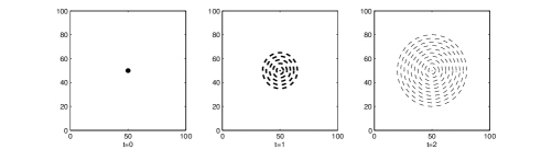
Figure 1: Signal Propagation

Since the action of PDE and diffusion away from the source cause the concentration of signal to decrease with distance from the signalling cell, we propose the following model to represent the signal strength that a cell receives from the source:

$$s_{i,j}=k_{1}\frac{r^{n}}{1+w\cdot d_{i,j}},$$ (IV.1)

where $i$ is the index of the focused cell, $j$ is the index of the signalling cell, $k_{1}$ is a scale factor, $r<1$ is the decaying factor due to the action of PDE, and $n$ is the time elapses after the firing, $w$ is a weight factor and $d_{i,j}$ is the Euclidean distance between cell $i$ and cell $j$. In the simulation we chose $k_{1}=1,r=0.95,w=0.038$. When $n>n_{0}$, the signal from this source is considered negligible. We chose $n_{0}=360$ in the simulation settings.

IV.2 Autonomous Firing

In Gregor’s experiment Gregor10 , the authors showed that “the stochastic pulsing of individual cells below the threshold concentration of extracellular cAMP plays a critial role in the onset of collective behavior”, and they showed that the firing rate changes from once every 15-30 minutes to once every 6 minutes. To simulate this behavior, we first set a base refractory time window to be 6 minutes (or 120 steps in the simulation). Beyond this period, an additional time window is added, whose length decreases with age. The length of this additional time window as a function of age is given by $twl(n)=ceil(320*(k_{2}-\arctan(k_{3}*(n-k_{4})/\pi)))$, where $k_{2}=0.473,k_{3}=0.001,k_{4}=7000$, and $n$ indicates time steps after starvation. Thus, the length of this additional time window decreases from 15 minutes at the beginning of simulation to about 0 by the end of the simulation, where $n=20000$ indicating approximately 16 hours and 36 minutes.

In the first step of simulation, the firing time spot of each cell is randomly chosen within a 30-min time window. After the first firing, a cell enters the refractory period whose time length equals $\max(120,twl(n))$. After this period, the firing time spot is randomly chosen within the time window $twl(n)$, if the cell is not stimulated.

IV.3 Signal Relaying

In each time step (or iteration), a cell accumulates the signal sent by other cells as described in Section IV.1. This accumulation is taken as the concentration of extracellular cAMP, and if it is below a threshold, say $thd_{1}$, the cell does not respond to it. If this concentration is above $thd_{1}$, and the cell is NOT in the refractory period, the cell responds to this signal by releasing a pulse of cAMP. This is known as signal relaying and thus the quorum sensing is formed. It is also known that a cell relays the signal only if it senses a wavefront of the stimulating signal Goldbeter96 . Thanks to the discrete model, this feature can be easily obtained by taking the difference of current and previous signal. If this difference is bigger than a threshold Song06 , $thd_{2}$, the cell is stimulated and relays the signal. In the numerical simulation, we set $thd_{1}=1.1$ and $thd_{2}=2.5\times 10^{-5}$. A time delay of 5 steps, indicating 15 seconds of time delay in response Mackay78 , is also incorporated before the release of cAMP of the stimulated cell.

The simulation code maintains a queue of the positions of all signal sources. If a cell fires at a certain position, that information is added into the queue. Associated with each entry of the queue there is a number indicating the lifetime of that signal. If the lifetime exceeds $n_{0}$, that signal is negligible and that entry is eliminated from the queue.

IV.4 Cell Movement

When the concentration of extracellular cAMP around a cell is below $thd_{3}$ (set at 2.42 in the simulation), the cell moves like random walk. In this case, a cell has two different ways of movements, namely the straight swim and tumble. To simulate this feature, we assume that with half of the chance the cell stays at the same position in the next step, and with equal probabilities (1/16) it moves to any of the neighboring points. In Gregor’s experiment Gregor10 , the cells were observed to fire synchronously 5 hours after starvation, and over the next 2 hours, the firing rate shortened to once every 6 minutes and the cells began to move. Therefore, it is reasonable to make $thd_{1}<thd_{3}$, i.e., the threshold of signal relaying is less than the threshold of chemotaxis so that synchronous firing precedes chemotaxis. This is different from the settings in Mackay78 .

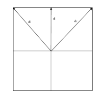
Figure 2: Moving directions

When the concentration of cAMP is above $thd_{3}$, the chemotaxis starts, and a cell moves in a way like purposeful random walk due to the two different movements. Although the advantage of continuous model is its capability to incorporate acceleration or deceleration, it is also possible to implement this feature into the discrete models by taking into account the inertia Nishimura05 .

IV.4.1 The Choice of Direction

We use a vector ${\bf d}$ to indicate the moving direction of a cell. If a cell is not stimulated, ${\bf d}=0$. In each iteration, the cell is assumed to be able to sense the difference of the signal coming from the neighboring points. Let $s_{1}\geq s_{2}$ be the strengths the two most strongest signal from the neighboring points, and ${\bf d}_{1},{\bf d}_{2}$ be their respective directions apart from the cell. $s=s_{1}{\bf d}_{1}\cdot s_{2}{\bf d}_{2}$ is computed. Notice that if strong signals coming from opposite directions, $s$ is still a small number. We take $s$ as the tendency to choose the direction ${\bf d}={\bf d}_{1}$, and we classify $s$ into ‘strong’, ‘medium’ and ‘weak’ according to the value of $s$. In each class of $s$, we assign a number $m_{i}$ to indicate the number of steps that the cell tends to move in the direction ${\bf d}$. In the simulation, we set $m_{1}=6$, $m_{2}=4$ and $m_{3}=2$ associated with the three classes of $s$, respectively. A 5-step time delay is implemented before the start of the movement of the cell, and this is the same time when the stimulated cAMP is released Mackay78 .

IV.4.2 The Purposeful Random Walk

After determined the moving direction ${\bf d}$ and the number of steps to move in that direction, the cell does not necessarily move straightly in that direction. Due to tumbling, the cell moves along a direction for a few steps and re-choose the direction. To incorporate this feature, we assume that in each time step, the cell moves along the direction ${\bf d}$ with a higher probability, but also with smaller probabilities to move along the neighboring directions ${\bf d}_{l},{\bf d}_{r}$ as shown in Fig. 2. After each step of movement, the direction ${\bf d}$ is updated to indicate the actual direction that the cell is going to follow. When the anticipated number of steps $m_{i}$ has reached, and there is no more stimulation during the movement, set ${\bf d}=0$ to indicate that the cell loses direction and will follow the random walk as being not stimulated.

IV.4.3 Acceleration, Deceleration and Steering

It is very obvious that while a cell is stimulated and performing the purposeful random walk, there are more signals received during the movement. The cell is assumed to be able to sense the signal at each time step. That is, in a certain time step, the cell moves along the direction ${\bf d}$, and senses new signal $s$ with the strongest signal coming from direction ${\bf d}_{1}$. We compare ${\bf d}$ and ${\bf d}_{1}$. If the angle between ${\bf d}$ and ${\bf d}_{1}$ is less than $90^{\circ}$, we take this new signal $s$ as a plus, and set ${\bf d}={\bf d}_{1}$ for the next step, also, according to the strength of $s$ we update the anticipated number of steps $m_{i}$. On the contrary, if the angle between ${\bf d}$ and ${\bf d}_{1}$ is greater than or equal to $90^{\circ}$, we take this new stimulus as a minus. This simulates the situation that, while a cell is moving in one direction, it senses a strong signal from the opposite direction. In this case, we reduce $m_{i}$ by some steps according to the strength of $s$. In other words, we reduce the number of anticipated steps that the cell originally tended to move in direction ${\bf d}$. Once $m_{i}$ is zero, ${\bf d}$ is set at zero, which means the cell is ready to choose a new direction once there is new stimulus.

V Simulation Result

We first randomly put 180 cells into the chamber to reproduce the experiment result done by Gregor et al Gregor10 . A plus symbol $+$ in the figure indicates the firing of a stimulated cell, which lasts for two steps (the release of cAMP is impulsive, but we draw the star for two steps in the iteration in order to observe it), and $t$ in the title is the index of time steps, where each step represents 3 seconds in the actual experiment.

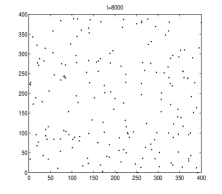
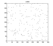
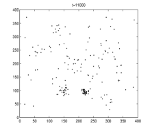
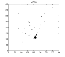
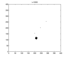
Figure 3: Amoebae Positions, 180 cells

When $t=6000$, synchronous firing is well detected, and when $t=8000$, the cells began to move. Because of the 15 seconds of delay in response time, it is not likely to see all the cells flashing at one particular shot. When $t=11000$ the cells form small groups which compete, and eventually all the cells aggregate.

We increase the number of cells to 380 and plot the clustering dynamics in Figure 4. As expected, more cells increase the concentration of extracellular cAMP more quickly, and the cells begin to aggregate at an earlier time.

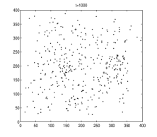
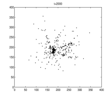
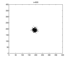
Figure 4: Amoebae Positions, 380 cells

100 trials are run and the aggregation positions with 180 cells and 380 cells, respectively, are drawn in Figure 5.

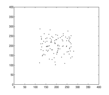
(a) 180 cells, 100 trials

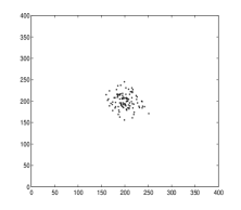
(b) 380 cells, 100 trials

Figure 5: Amoebae Aggregation Centers

We can see from Figure 5 that when there are more cells, the aggregation center is closer to the center of the chamber, while less cells make the aggregation center deviated.

The number of cells is increased from 180 to 380 by 25 each time. For each setting, 100 trials are run and the average aggregation time, variance of aggregation time and variance of aggregation location are plotted in Figures 6, 7 and 8, respectively.

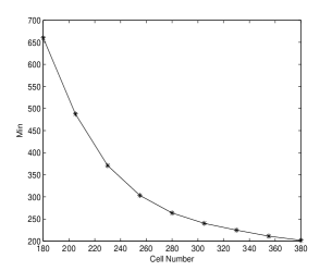
Figure 6: Mean Aggregation Time

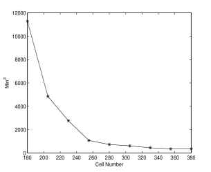
Figure 7: Variance of Aggregation Time

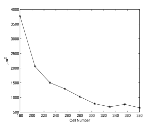
Figure 8: Variance of Aggregation Location

As expected, more cells shortened the aggregation time. However, after the point 280, the curves in Figures 6, 7 and 8 all flatten out. Since synchronous firing plays the key role in quorum sensing, the procedure from sporadic firing to synchronous firing is important for the clustering dynamics of social Amoebae. Even though more cells increase the extracellular cAMP more quickly, they do not necessarily aggregate sooner if the firing are not well paced. Gregor et al Gregor10 showed that the sporadic firing below the threshold concentration of cAMP plays a critical role in the onset of the collective behavior of social Amoebae, and we believe that the role which sporadic firing plays is to make the firing well paced. Therefore, the way the signal propagates in the media is critical in the clustering dynamics, and this feature is often missed in most continuous models.

To further study the effect of signal propagation, we set the number of cells at 380 and set the parameter $w=0.08$ in (IV.1). This mimics the situation where the signal decays faster with distance from the source.

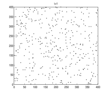
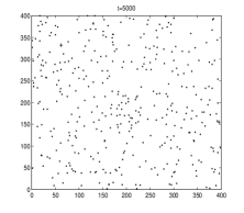
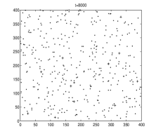
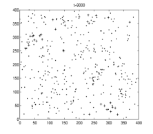
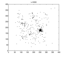
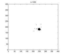
Figure 9: Amoebae Positions, 380 cells, $w=0.08$

As can be seen from Figure 9, the cells tend to form small groups that compete and the firing are not well paced, and as a consequence, the cells take longer time to aggregate.

VI Concluding Remarks

In this paper, we present a discrete model for computer simulations of the clustering dynamics of Social Amoebae. This model incorporates the wavelike propagation of extracellular signaling cAMP, the sporadic firing of cells at early stage of aggregation, the signal relaying as a response to stimulus, the inertia and purposeful random walk of the cell movement. The simulation result of this model could well reproduce the phenomenon observed by actual experiments. We found that synchronous firing plays a critical role in the clustering dynamics of social Amoebae. The sporadic firing at early stage after starvation is necessary to obtain the synchronous firing preceding the aggregation. A Monte Carlo simulation is run which shows the existence of potential equilibriums of mean and variance of aggregation time.

As a future research topic, it might be interesting and necessary to take into account the volume of each cell, and the change of shape as a cell moves Nishimura05 . In that case, we anticipate that the cells are easier and faster to aggregate.

References

- (1) J.C. Dallon and H.G. Othmer, A Discrete Cell Model with Adaptive Signalling for Aggregation of Dictyostelium discoideum, Phil. Trans. R. Soc. Lond. B(352) pp. 391–417, 1997.
- (2) A. Goldbeter, Biochemical Oscillations and Cellular Rhythms, Cambridge University Press, 1996.
- (3) T. Gregor, K. Fujimoto, N. Masaki and S. Sawai, The Onset of Collective Behavior in Social Amoebae, Science 328 pp. 1021–1025, 2010.
- (4) T. Hillen and K.J. Painter, A User’s Guide to PDE Models for Chemotaxis, J. Math. Biol. 58 183 pp. 183–217, 2009.
- (5) T. Höfer, J.A. Sherratt and P.K. Maini, Dictyostelium discoideum: Cellular Self-organization in an Excitable Biological Medium, Proc. R. Soc. Lond. B 259 pp. 249–257, 1995.
- (6) D. Ishii, K.L. Ishikawa, T. Fujita and M. Nakagawa, Stochastic Modeling for Gradient sensing by Chemotactic Cells, Sci. Technol. Adv. Mat. 5 pp. 715–718, 2004.
- (7) D.A. Kessler and H. Levine, Pattern Formation in Dictyostelium via the Dynamics of Cooperative Biological Entities, Phys. Rew. E 48 pp. 4801–4804, 1993.
- (8) H. Levine, Modeling Spatial Patterns in Dictyostelium, Chaos 4(3) pp. 563–568, 1994.
- (9) S.A. Mackay, Computer Simulation of Aggregation in Dictyostelium discoideum, J. Cell Sci. 33 pp. 1–16, 1978.
- (10) S.I. Nishimura and M. Sasai, Inertia of Amoebic Cell Locomotion as an Emergent Collective Property of the Cellular Dynamics, Phys. Rew. E 71 pp. 010902-1–010902-4, 2005.
- (11) C.A. Parent and P.N. Devreotes, A Cell’s Sense of Direction, Science 284 pp. 765–770, 1999.
- (12) C.A. Parent and A. Bagorda, Eukaryotic Chemotaxis at a Glance, J. Cell Science 121 (16) pp. 2621–2624, 2008.
- (13) A. Robertson and D.J. Drage, Stimulation of Late Interphase Dictyostelium discoideum Amoebae with an External Cyclic AMP Signal, Biophys. J. 15 pp. 765–775, 1975.
- (14) L.A. Segel, A Theoretical Study of Receptor Mechanisms in Bacterial Chemotaxis, SIAM J. Appl. Math., 32 pp. 653–665, 1977.
- (15) J.A. Sherratt, Chemotaxis and Chemokinesis in Eukaryotic Cells: the Keller-Segel Equations as an Approximation to a Detailed Model, Bull. Math. Biol. 56 pp. 129–146, 1994.
- (16) F. Siegert, C.J. Weijer, A. Nomura and H. Miike, A Gradient Method for the Quantitative Analysis of Cell Movement and Tissue Flow and Its Application to the Analysis of Multicellular Dictyostelium Development, J. Cell Sci. 107 pp. 97–104, 1994.
- (17) L. Song, et al, Dictyostelium discoideum Chemotaxis: Threshold for Directed Motion, European Journal of Cell Biology, 85 pp. 981–989, 2006.
- (18) P.J.M. van Haastert and P.N. Devreotes, Chemotaxis: Signalling the Way Forward, Nat. Rev. Mol. Cell Biol. 5 pp. 626–634, 2004.