A rotating molecular disk toward IRAS 18162–2048,
the exciting source of HH 80–81

ABSTRACT

We present several molecular line emission arcsec and subarcsec observations obtained with the Submillimeter Array (SMA) in the direction of the massive protostar IRAS 18162–2048, the exciting source of HH 80–81.

The data clearly indicates the presence of a compact (radius$\approx 425$–850 AU) SO₂ structure, enveloping the more compact (radius$\lesssim$150 AU) 1.4 millimeter dust emission (reported in a previous paper). The emission spatially coincides with the position of the prominent thermal radio jet which terminates at the HH 80–81 and HH 80N Herbig–Haro objects. Furthermore, the molecular emission is elongated in the direction perpendicular to the axis of the thermal radio jet, suggesting a disk–like structure. We derive a total dynamic mass (disk–like structure and protostar) of 11–15 M_☉. The SO₂ spectral line data also allow us to constrain the structure temperature between 120–160 K and the volume density $\gtrsim 2\times 10^{9}$ cm^-3. We also find that such a rotating flattened system could be unstable due to gravitational disturbances.

The data from C¹⁷O line emission show a dense core within this star–forming region. Additionally, the H₂CO and the SO emissions appear clumpy and trace the disk–like structure, a possible interaction between a molecular core and the outflows, and in part, the cavity walls excavated by the thermal radio jet.

1. INTRODUCTION

The powerful radiation from high-mass protostars was the main obstacle for understanding the formation of massive stars (see e.g. Larson & Starrfield 1971; Kahn 1974; Yorke & Kruegel 1977; Beech & Mitalas 1994; see also the recent review of Zinnecker & Yorke 2007). It was thought that the strong radiation pressure from the protostar would stop the accretion, hence preventing the formation of stars with masses over $\sim$10 M_☉. Although this theoretical problem can be overcome (e.g., Wolfire & Cassinelli 1987; Nakano 1989; Jijina & Adams 1996; Yorke & Sonnhalter 2002; Norberg & Maeder 2000; McKee & Tan 2003; Krumholz et al. 2005), it remains yet unclear how these stars are actually formed. There are several hypotheses for the formation process. Perhaps the most important ones are: (1) large accretion rates (3 or 4 orders of magnitude greater than those observed in low-mass protostars) through circumstellar disks (Walmsley 1995; Jijina & Adams 1996; McKee & Tan 2003; Zhang 2005; Banerjee & Pudritz 2007), (2) competitive accretion between small protostars of the same cluster, that could result in eventual mergers (Bonnell et al. 1998; Clarke & Bonnell 2008; Moeckel & Clarke 2011; Baumgardt & Klessen 2011), and (3) accretion of ionized material, even after the formation of a compact HII region generated by the protostar (Keto 2002; Keto & Wood 2006).

Table 1Spectral observations

Transition	$\nu_{line}$	$E_{u}$	Data	Synthesized Beam		RMS	Figures
	(GHz)	(K)		$\arcsec\times\arcsec$	$\arcdeg$	(Jy beam-1)
SO2 163,13–162,14	214.689380	147.9	LR	$8\farcs 3\times 3\farcs 1$	34.2	0.065	10
			ROB	$1\farcs 3\times 0\farcs 9$	59	0.085	8
			HR	$0\farcs 7\times 0\farcs 4$	13.2	0.085	9
SO2 176,12–185,13	214.728330	229.1	LR	$8\farcs 3\times 3\farcs 1$	34.2	0.065	10
SO2 64,2–73,5	223.883569	58.6	LR	$7\farcs 9\times 3\farcs 0$	34.2	0.065	10
SO2 202,18–193,17	224.264811	207.9	LR	$7\farcs 9\times 3\farcs 0$	34.2	0.065	10
SO2 132,12–131,13	225.153702	93.1	LR	$7\farcs 9\times 2\farcs 9$	34.2	0.065	10
			ROB	$1\farcs 2\times 0\farcs 9$	58	0.070	8
			HR	$0\farcs 7\times 0\farcs 4$	12.9	0.080	9
SO $7_{8}$–$7_{7}$	214.357004	81.3	LR	$8\farcs 3\times 3\farcs 1$	34.2	0.065	10
SO $5_{5}$–$4_{4}$	215.220653	44.1	LR	$8\farcs 2\times 3\farcs 1$	34.2	0.070	10
			ROB	$1\farcs 2\times 0\farcs 9$	58	0.080	8
			TAP	$4\farcs 0\times 2\farcs 2$	36.7	0.080	3,2,4
C17O 2–1	224.714385	16.2	LR	$7\farcs 9\times 2\farcs 9$	34.2	0.075
			TAP	$4\farcs 0\times 2\farcs 1$	37.8	0.080	1
H2CO 31,2–21,1	225.697775	33.5	LR	$7\farcs 9\times 2\farcs 9$	34.2	0.090	10
			ROB	$1\farcs 2\times 0\farcs 9$	58	0.100	8
			TAP	$4\farcs 0\times 2\farcs 1$	37.2	0.095	6,5,4

Note. — Data extracted from JPL catalogue. The fourth column Data is a code giving the resolution of each map. LR means low angular resolution data, HR, high angular resolution data, ROB, combined images with the robust set to 0.3 and TAP, combined images with a taper applied and restricted in the uvplane (see text, section §2).

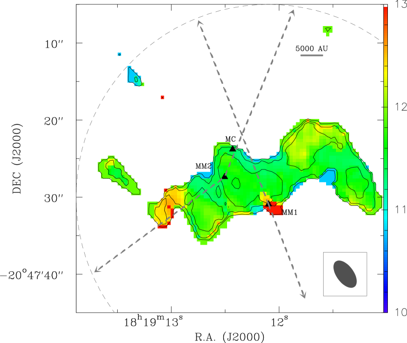
Figure 1.— Contour image of the zero order moment superposed on the first order moment colour image of the C¹⁷O 2–1 line emission (combined compact and extended configuration data with a Gaussian uv taper) toward IRAS 18162–2048. Contour levels are -9, -4, 4, 9, 15, 30, 45, 60, 75 and 90 times 0.10 Jy beam^-1 km s^-1, the rms of the image. The units of the scale bar are in  km s^-1. The molecular emission is integrated over velocities between 9 and 18 km s^-1. The triangles mark the position of the millimeter sources MM1 and MM2, and the position of the molecular core, MC. The dashed arrows show the directions of the NW and SE outflows which seem to originate at the MM2 position and also the NE-SW thermal radio jet, launched from MM1. The synthesized beamsize is shown at the bottom right corner and the primary beam is indicated by the dashed circle.

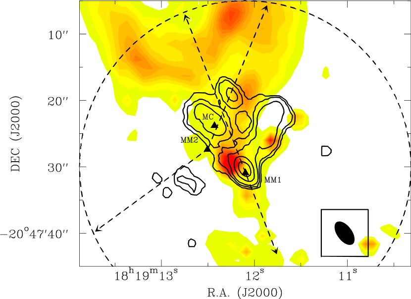
Figure 2.— Contour image of the zero order moment of the SO $5_{5}$–$4_{4}$ line emission (combined compact and extended configuration data with a Gaussian uv taper) superimposed on a K–band near infrared image of the reflection nebula in the IRAS 18162–2048 region (courtesy of Thomas Geballe; see Aspin & Geballe 1992). The infrared polarimetric study carried out by Yamashita et al. (1987) demonstrated that the scattered light from the infrared reflection nebula occurs on grains at the walls of a parabolic cavity rather than on grains inside the whole outflow lobe. Contour levels are -9, -4, 4, 9, 15, 30, 45, 60, 75 and 90 times 0.17 Jy beam^-1 km s^-1, the rms of the image. Symbols are as in Fig. 1.

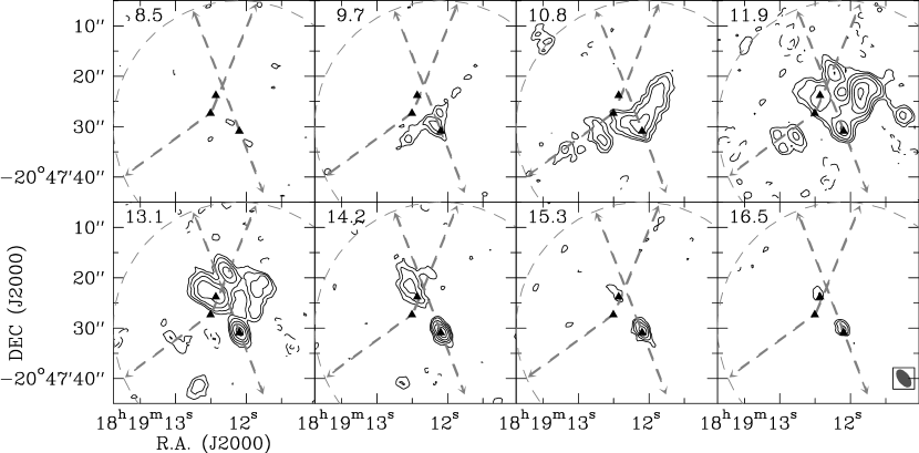
Figure 3.— Channel velocity image of the SO $5_{5}$–$4_{4}$ extended emission (combined compact and extended configuration data with a Gaussian uv taper) from the central region of IRAS 18162–2048. The emission is averaged in velocity bins of 1.14 km s^-1. The velocity of each channel is indicated in the top left corner of each panel in  km s^-1 units. The cloud velocity is at about 11.8 km s^-1. The contour levels are -6, -4, 4, 6, 9, 13, 18, 24, 31, 39, 48 and 58 times 0.08 mJy beam^-1, the rms of the image. Symbols are as in Fig. 1. The synthesized beam size is shown in the bottom left-hand corner of the most redshifted channel. The blueshifted emission appears to trace mainly the walls of the cavity excavated by the radio jet from MM1. At the position of MM1 the image shows emission probably coming from the rotating disk/ring, absorbed in the bluest channels by the extended emission. The redshifted channels show also compact emission toward the position of MC.

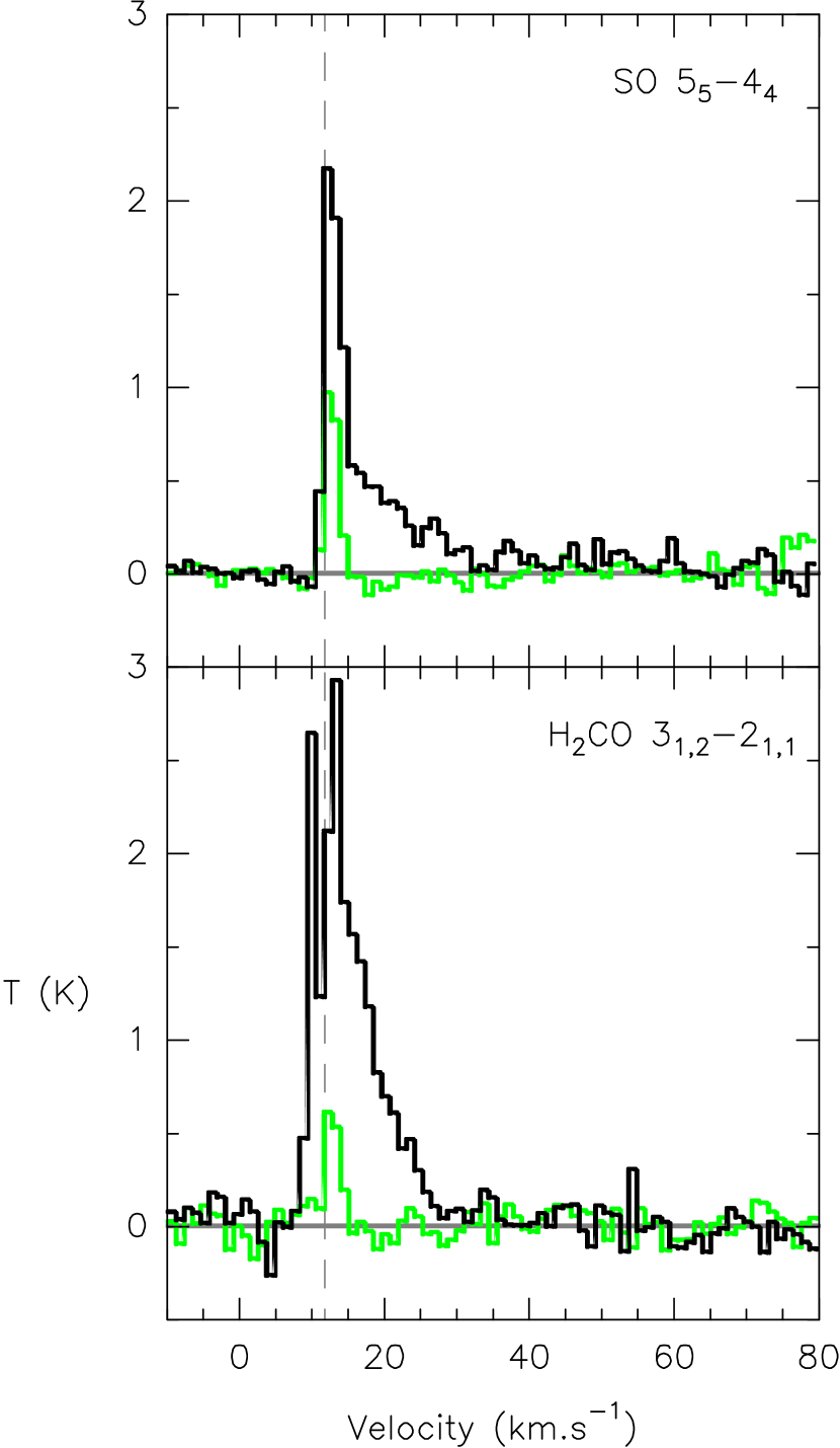
Figure 4.— SO $5_{5}$–$4_{4}$ (top panel) and H₂CO 3_1,2–2_1,1 (bottom panel) spectra toward the center position of MC (black line). Spectra toward the clump located to the north–west of MC (green line) are included to compare with that of MC. The dotted line marks the systemic velocity (11.8 km s^-1). The intensity is in Kelvin. The spectra are extracted from the combined compact and extended configuration data with a Gaussian uv taper.

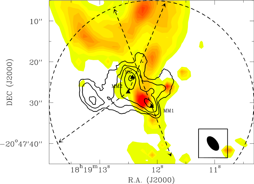
Figure 5.— Contour image of the zero order moment of the H₂CO 3_1,2–2_1,1 line emission (combined compact and extended configuration data with a Gaussian uv taper) overlaid with a K–band near infrared image of the IRAS 18162–2048 region (as shown in Fig. 2). Contour levels are -9, -4, 4, 9, 15, 30, 45, 60, 75 and 90 times 0.33 Jy beam^-1 km s^-1, the rms of the image. Symbols are as in Fig. 1.

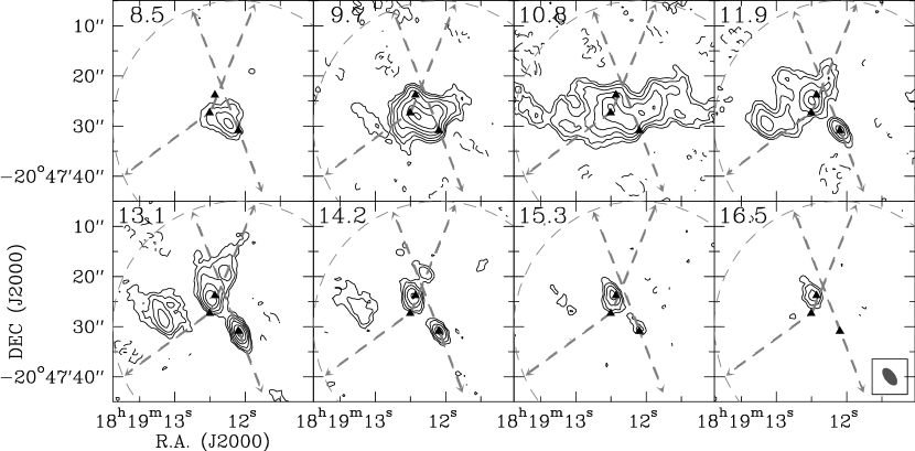
Figure 6.— Channel velocity image of the H₂CO 3_1,2–2_1,1 extended emission (combined compact and extended configuration data with a Gaussian uv taper). The emission is averaged in velocity bins of 1.14 km s^-1. The velocity of each channel is indicated at the top left corner of each panel in  km s^-1 units. The cloud velocity is at about 11.8 km s^-1. The contour levels are -6, -4, 4, 6, 9, 13, 18, 24, 31, 39, 48 and 58 times 0.095 mJy beam^-1, the rms of the image. Symbols are as in Fig. 1.

In recent years, several works have provided evidence for the presence of collimated jets (HH 80-81, Martí et al. 1993; Cep A, Curiel et al. 2006; IRAS 23139, Trinidad et al. 2006; IRAS 16547, Rodríguez et al. 2008), molecular outflows (see a summary in Zhang 2005; Arce et al. 2007), and flattened structures of dust and gas (some with rotation and some with infall signposts; e.g., Cep A, Patel et al. 2005; IRAS 20126, Cesaroni 2005; AFGL 2591, van der Tak et al. 2006; W51 North, Zapata et al. 2008; IRAS 16547, Franco-Hernández et al. 2009; W33A-MM1, Galván-Madrid et al. 2010), surrounding high-mass protostars. The evidence leads to the interpretation that massive star formation is analogous to low-mass star formation, that is, via accretion from a flat rotating disk, with a jet of ionized material, and with an associated molecular outflow. However, the physical characteristics of the possible accretion disks and their associated outflows have not been well characterized yet. Hence, the formation process of massive stars remains an open issue. There are several problems that hamper the analysis of massive star formation regions (MSFRs). First, massive protostars form in clusters, which together with projection effects, make these regions difficult to interpret. Moreover, the MSFRs are found at larger distances than low-mass star formation regions, with typical distances of 2-5 kpc. Thus, to get an insight of the closest regions to the protostars, where accretion disks are expected, the highest angular resolution of the current telescopes is needed. Even so, most of the dust and gas structures detected around high-mass protostars are $\sim 1000$ AU. This is the smallest diameter that an interferometer can resolve with a 1$\arcsec$ angular resolution at those distances. At these scales, such structures could harbour systems of several protostars, that could be forming high mass stars by other mechanisms such as mergers. In fact, the nearest massive protostars (Orion BN/KL and Cepheus A HW2), show complex scenarios, with a possible merger of protostars (Orion BN/KL, Zapata et al. 2009), or close passages between protostars (Cep A HW2, Cunningham et al. 2009). Therefore, with the current interferometers, only a few MSFRs may be studied with adequately high angular resolution.

To demonstrate the existence of a disk around a massive protostar, it is not enough to detect its (sub)millimeter dust continuum emission; its kinematics must also be measured via the molecular line emission associated with the gas–phase chemistry developed after the evaporation of the molecules from the ice mantles (Hatchell et al. 1998; Cesaroni et al. 2007). However, searching for molecular tracers of disks in MSFRs is a complex task. There are molecules that show emission from the envelope and the disk simultaneously. Other molecules show optically thick emission, thus complicating the kinematic study of the disk. On the other hand, S-bearing species (such as H₂S, SO, SO₂, CS, OCS…) could be intimately linked with the evaporation process of the disk surface (Charnley 1997; Hatchell et al. 1998; van der Tak et al. 2003; Martín-Pintado et al. 2005), becoming good tracers of the dynamics of the innermost parts of the high mass protostars. Recently, several papers have been published on the detection of S-bearing species in disks and other warm gas-structures of MSFRs (van der Tak et al. 2006; Jiménez-Serra et al. 2007; Klaassen et al. 2009; Franco-Hernández et al. 2009; Zapata et al. 2009). In particular, SO₂ transitions, ubiquitous within the (sub)millimeter range, show a very compact nature, suggesting their close association with circumstellar structures.

The GGD27 complex is an active star forming region located at a distance of 1.7 kpc. It shows a spectacular (5.3 pc long) and highly collimated thermal radio jet (Martí et al. 1993, 1995, 1998), embedded within a powerful CO bipolar outflow (Yamashita et al. 1989; Benedettini et al. 2004). The jet has a position angle of $\sim 21\arcdeg$ (Martí et al. 1993, 1999) and ends at two southern and very bright Herbig-Haro objects (HH 80 and 81, originally discovered by Reipurth & Graham 1988) and at a radio source to the north (HH 80 North, Girart et al. 1994). Linear polarization has been detected in the radio emission from this jet, indicating the presence of a magnetic field coming from the disk (Carrasco-González et al. 2010).The central part of the radio jet has a bright far-infrared counterpart (IRAS 18162–2048), that implies the presence of a luminous young star ($\sim 2\times 10^{4}$ L_☉) or a cluster of stars (Aspin & Geballe 1992; Stecklum et al. 1997).

Submillimeter and millimeter wavelength observations of the central part of the thermal radio jet have revealed two dusty sources, MM1 and MM2, separated by about 7$\arcsec$ (Gómez et al. 2003; Qiu & Zhang 2009), which are apparently in very different evolutionary stages (Fernández-López et al. 2011, hereafter Paper I). MM1, the south-western source, coincides with the origin of the thermal radio jet and has a dust temperature of 109 K. It has a weak extended envelope, possibly surrounding a very compact (R$\lesssim$150 AU) disk-protostar system. The mass of the disk derived from the continuum emission is $\sim 4.1$  M_☉. Such a massive disk could have an extremely high accretion rate ($10^{-3}-10^{-2}$ M_☉ yr^-1). However, the case for an accretion disk in MM1 has not been unambiguously confirmed yet. The bolometric luminosity obtained from fitting the SED of high angular resolution data is $\geq 3300$ L_☉, similar to that of a B1 Zero Age Main Sequence (ZAMS) star. However, the massive disk of MM1 (compared to those of low-mass protostars), the presence of the powerful outflow and the youth of the protostar (it has not developed a compact H II region yet), indicate that MM1 could become a B0 or a more massive star. MM1 is also associated with compact emission from several high density tracers, such as CS (Yamashita et al. 1991), SO (Gómez et al. 2003), CH₃OH, CH₃CN, H${}_{2}^{13}$CO, OCS, HNCO and SO₂ (Qiu & Zhang 2009).

The physical characteristics of MM2 are typical of the Class 0 low–mass protostars (see e.g., Andrè et al. 1993), except for its total mass of at least 11 M_☉ (4-5 times more mass than a typical low-mass Class 0 source, see e.g. Girart et al. 2006; Rao et al. 2009). MM2 appears as an extended source when observed with low angular resolution at 1.4 mm, but it is separated into two compact sources when observed with high angular resolution (Paper I). The stronger component in MM2 spatially coincides with very weak free-free emission, suggesting that it could be a high/intermediate mass protostar. The weaker component in MM2 could be a pre-protostellar core. Previous CO observations (Qiu & Zhang 2009) have associated the position of MM2 with the origin of a young outflow running to the east. In addition, another possible CO outflow, running north-west of MM2 could also have originated close to this position.

There is also a possible molecular core (hereafter MC, Qiu & Zhang 2009) located about $4\arcsec$ to the north-west of MM2. Although MC is traced by several molecules (CH₃CN, H${}_{2}^{13}$CO, OCS y HNCO, Qiu & Zhang 2009, and a Class I CH₃OH maser, Kurtz et al. 2004), it is not associated with a bright and compact millimeter source (Paper I). The diverse line emission from MC has been interpreted by Qiu & Zhang (2009) as the emission from a hot core warmed by the radiation of a young and massive protostar.

Here we present an analysis of the molecular emission of several lines (mostly S-bearing species) detected in the central region of IRAS 18162–2048 using the Submillimeter Array (SMA; Ho et al. 2004). The SMA allowed us to detect several transitions simultaneously, some of which seem to trace a circumstellar disk/ring around MM1, with subarcsecond resolution ($\sim 0\farcs 5$), permitting a beam size of $\sim 850$ AU at the source distance. This resolution is necessary in order to perform a reliable kinematical analysis of the motions of the circumstellar disks at distances greater than 1–2 kpc.

The continuum emission of the observations was presented in a recent publication (Paper I). In section 2 we briefly describe the observations, while in section 3 the results of the observations are given. Section 4 contains the analysis of the column density and the temperature of the disk/ring of MM1, followed by a discussion in section 5. Finally, in section 6 we draw our main conclusions.

2. OBSERVATIONS

The SMA observations were taken during two epochs: on 2005 August 24 in the compact configuration (giving a synthesized beam of $8\farcs 1\times 3\farcs 0$) and on 2007 May 27 in the very extended configuration (giving a synthesized beam of $0\farcs 7\times 0\farcs 4$). During both epochs the receiver was tuned at 215/225 GHz. The phase center of the telescope was RA(J2000.0)$=18^{h}19^{m}12\fs 1$ and DEC(J2000.0)$=-20\arcdeg 47\arcmin 30\farcs 0$, and the correlator provided a spectral resolution of about 1.14 km s^-1 at the observed frequency (with 0.81 MHz of channel width). The continuum data were edited and calibrated using Miriad (Sault et al. 1995). The flux uncertainty was estimated to be $\sim 20$%. The detailed description of the observing setup as well as the calibration process of the continuum emission data can be found in Paper I.

Nine emission lines were detected with the compact configuration (Table 1), four of which were also detected with the very extended configuration (SO₂ 16_3,13–16_2,14, SO₂ 13_2,12–13_1,13, SO $5_{5}$–$4_{4}$, H₂CO 3_1,2–2_1,1). The solutions of the self–calibration performed on the continuum data were transferred to the line data, and then the molecular lines were imaged, cleaned, restored, and analyzed using the Miriad and AIPS (developed by NRAO) packages. The line data were also corrected for the half-channel error in the SMA velocity labeling discovered in 2007 November. After that, we used a channel separation of 1.136 km s^-1 for all the lines. The calibration was performed in the same manner for the compact and very extended configuration data, except for the flux calibration step (see Paper I). Finally, the two data sets (compact and very extended configurations) were combined for all the lines giving maps with an intermediate angular resolution (hereafter combined data). The average rms noise level is $\sim$70 mJy beam^-1 in the line channel maps obtained with the compact configuration data, $\sim$85 mJy beam^-1 in those obtained with the very extended configuration, and $\sim$85 mJy beam^-1 in those obtained with the combined data, all with a natural weighting. Throughout the paper, all the velocities are given in LSR.

We use the high angular resolution data (very extended configuration) to analyze the disk kinematics and the low angular resolution data (compact configuration) to extract the spectra and estimate the disk temperature and column density. In addition, we obtain two different sets of images using the combined data to examine the extended emission with different angular resolutions. First, we set the robust parameter to 0.3. It yields a synthesized beam of about $1\farcs 2\times 0\farcs 9$ (Table 1). Second, we apply a taper of 182 k$\lambda$ and restrict the visibilities up to 200 k$\lambda$, thus improving the sensitivity to the extended emission. The synthesized beam of the tapered data is about $4\farcs 0\times 2\farcs 1$ (see Table 1).

3. RESULTS

Table 2Gaussian fits to the low angular resolution data toward MM1.

Line	$S_{\mathrm{peak}}$	VLSR	FWHM	Gaussian area	RMS	Zero-to-zero
	K	km s-1	km s-1	K km s-1	K	km s-1
SO2 163,13–162,14	$1.32\pm 0.03$	$13.04\pm 0.05$	$5.9\pm 0.2$	$8.2\pm 0.4$	0.03	5.5-19.0
SO2 132,12–131,13	$1.33\pm 0.05$	$12.9\pm 0.1$	$6.0\pm 0.4$	$8.5\pm 0.4$	0.07	6.5-18.0
SO2 176,12–185,13	$0.56\pm 0.05$	$13.2\pm 0.3$	$5.7\pm 0.4$	$3.4\pm 0.8$	0.06	8.5-20.0
SO2 202,18–193,17	$0.88\pm 0.05$	$12.8\pm 0.2$	$6.6\pm 0.4$	$6.2\pm 0.7$	0.06	6.0-19.0
SO2 64,2–73,5	$0.49\pm 0.05$	$13.4\pm 0.2$	$6\pm 0.5$	$3.3\pm 0.7$	0.05	6.5-20.0
SO $5_{5}$–$4_{4}$	$2.29\pm 0.04$	$12.86\pm 0.04$	$5.65\pm 0.05$	$13.8\pm 0.5$	0.04	6.0-19.0
SO $7_{8}$–$7_{7}$	$0.5\pm 0.1$	$9.8\pm 0.3$	$3\pm 0.5$	$1.3\pm 0.4$	0.07	6.5-18.0
	$0.63\pm 0.05$	$13.8\pm 0.3$	$4\pm 0.5$	$2.5\pm 0.4$
H2CO 31,2–21,1	$3.6\pm 0.1$	$9.72\pm 0.05$	$2.1\pm 0.1$	$8.3\pm 0.6$	0.10	5.0-17.0
	$3.7\pm 0.1$	$13.10\pm 0.05$	$2.6\pm 0.2$	$6.56\pm 0.6$

Note. — The spectra were obtained over a box (-8,-8,7,7) arcsecs. Gaussian fits were carried out with a program based on the algorithm by Cantó et al. 2009.

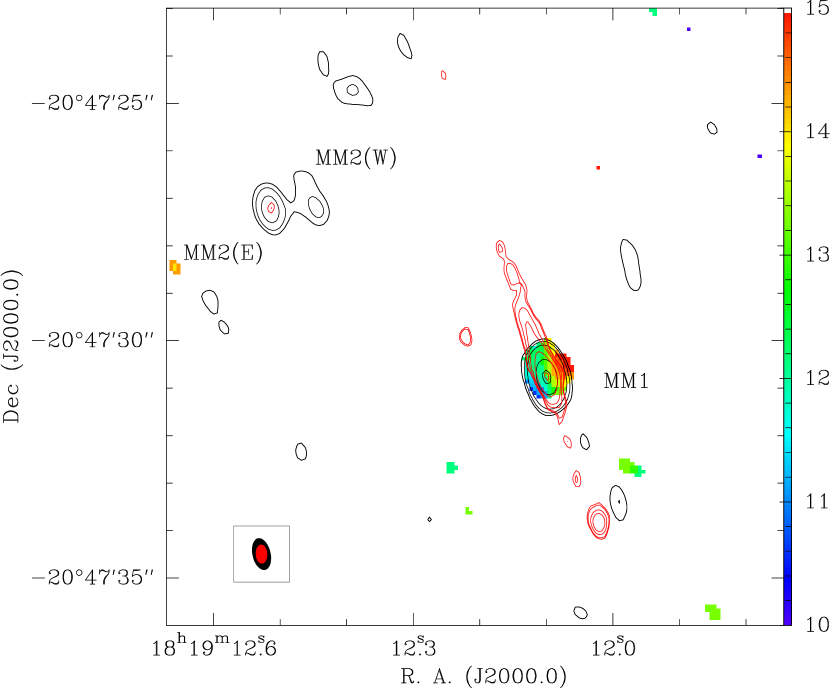
Figure 7.— Image of the VLA radio continuum emission at 3.5 cm (red contours), SMA 1.4 mm continuum emission (black contours) and the SMA integrated emission of the SO₂ 13_2,12–13_1,13 line (colour scale). The contour levels of the 3.5 cm map are 5, 6, 10, 15, 40 and 200 times 8.8 $\mu$mJy beam^-1, the rms of this image. The contour levels of the 1.4 mm image are -5, 3, 3, 5, 10, 60 and 120 times 0.003 mJy beam^-1, the rms of this image. The SO₂ 13_2,12–13_1,13 molecular emission is integrated over the velocity range 7–19 km s^-1, and the wedge panel in the right shows the colour scale intervals. In the bottom left corner the synthesized beams of the cm image (red ellipse) and the mm images (black ellipse) are shown.

3.1. C¹⁷O emission

Fig. 1 shows the integrated emission of the C¹⁷O 2–1 molecular line superposed on the first order moment. The C¹⁷O emission extends mainly along a south–east to north–west lane of $\sim 23\arcsec\times 10\arcsec$ ($\sim 0.2$ pc $\times$ 0.1 pc) and a position angle of $\sim 120\arcdeg$, approximately perpendicular to the thermal radio jet (position angle of 21$\arcdeg$). The two main peaks of the C¹⁷O 2–1 emission appear on both sides of the thermal radio jet (see Fig. 1), with the strongest peak at a position between the two dominant (sub)millimeter sources, MM1 and MM2. MM1 (the source from which the radio jet is launched), is located at the bottom center of the C¹⁷O 2–1 lane emission.

Fig. 1 also shows that the v_LSR of the line is almost constant along the lane structure. The line is narrow and has a symmetric profile, with a full width at half maximum (FWHM) of 2.8 km s^-1 $\pm 0.03$. A Gaussian fit to this line profile gives also a central velocity of 11.8$\pm$0.03 km s^-1. In what follows we will consider this value as the systemic velocity. This velocity agrees well, to within our spectral resolution, with that measured by Gómez et al. (2003) (12.2$\pm$0.1 km s^-1) from the emission of the ammonia core.

The critical density of the C¹⁷O 2-1 line is relatively low, $n_{\rm crit}\sim 10^{4}$cm^-3,so we expect that the emission detected by the SMA is likely thermalized. Assuming LTE conditions will yield a lower limit for the total mass of the extended molecular cloud. We assume a C¹⁷O abundance of $4.7\times 10^{-8}$ (Frerking et al. 1982) and an excitation temperature of 24 K, equal to the T_rot found by Gómez et al. (2003) using the NH₃ VLA observations. From equations B1 and B2 of Frau et al. (2010) and for optically thin emission, we obtain an average molecular column density of $7\times 10^{22}$ cm^-2. Hence, we estimate a lower limit of 38 M_☉ for the total mass.

3.2. SO emission

The SMA correlator setting includes two SO transitions: SO $7_{8}$–$7_{7}$ and SO $5_{5}$–$4_{4}$. We detect SO $7_{8}$–$7_{7}$ only in the compact configuration due to a problem with the correlator at the frequency of this line in the very extended configuration. The SO $7_{8}$–$7_{7}$ line emission from the compact configuration data appears as an unresolved clump toward MM1. On the other hand, the emission from the SO $5_{5}$–$4_{4}$ line at the systemic velocity of the dense core shows a clumpy distribution mainly to the north of MM1, having a conical shape which surrounds the north lobe of the thermal radio jet (Figs. 2 and 3). Some of the weaker clumps seem to coincide with the direction of the north–west and south–east outflows observed by Qiu & Zhang (2009). The redshifted emission (with respect to the cloud velocity) is compact and is mainly distributed around MM1 and MC (Fig. 3). The SO $5_{5}$–$4_{4}$ line profile at the position of MC (top panel of Fig. 4) has associated a clear redshifted wing with emission spreading up to a few tens of km s^-1.

3.3. H₂CO emission

The emission of the H₂CO 3_1,2–2_1,1 line is more extended than that of the SO $5_{5}$–$4_{4}$ line, resembling the distribution of the elongated C¹⁷O 2–1 emission around the systemic velocity (Fig. 5 and 6). Furthermore, at the 11.9 and 13.1 km s^-1 velocity channels the emission appears to follow the direction of the two outflows mentioned above. At redshifted velocities ( $v_{\rm LSR}$  $\gtrsim 13.1$ km s^-1) the emission is mainly distributed around the north lobe of the radio jet, similarly to that observed in the SO redshifted emission. Contrary to the SO, the H₂CO 3_1,2–2_1,1 presents emission around MM 2. On the other hand and as occurs with the SO, the H₂CO 3_1,2–2_1,1 emission is enhanced at the positions of MM1 and MC. Toward MC, the H₂CO 3_1,2–2_1,1 line shows a high velocity red wing, more prominent than that observed in SO $5_{5}$–$4_{4}$ line profile (bottom panel of Fig. 4).

3.4. SO₂ emission

Five SO₂ lines were detected with the SMA in its compact configuration (Table 2). All of them show unresolved emission at the origin of the thermal radio jet, which coincides with the MM1 (sub)millimeter continuum source (Fig. 7). SO₂ 16_3,13–16_2,14 and SO₂ 13_2,12–13_1,13 were also detected by the SMA in its very extended configuration. The other SO₂ lines were undetected due to their low intensity, their (probably) partially resolved nature and the lower sensitivity of the high angular resolution data. The panels a) and b) of Fig. 8 show the velocity channel cubes of the SO₂ 16_3,13–16_2,14 and SO₂ 13_2,12–13_1,13 lines (images of the combined data with robust 0.3). The molecular structure at the position of MM1 appears at the 8.7 km s^-1 to 15.6 km s^-1 velocity channels, while the peak velocity is  $v_{\rm LSR}$ $\simeq 13.0$ km s^-1 (see Table 2). The peak velocity of the molecular structure is therefore redshifted with respect to the large scale dense core velocity by $\sim 1.2$ km s^-1. The blueshifted channels (8.7 to 11.0 km s^-1) are seen to the east, while the redshifted channels (14.4 and 15.6 km s^-1) are seen to the west with respect to the thermal radio jet and the 1.4 mm continuum peak position.

Table 3Size and kinematics of the SO₂ disk. From the high angular resolution data.

Line	Deconvolved Size			R	Vdisp	$\Theta_{\rm disp}$	Mdyn
	$\arcsec$	$\arcsec$	$\arcdeg$	AU	km s-1	M☉	M☉
SO2 163,13–162,14	$0.88\pm 0.08$	$0.81\pm 0.05$	$130\pm 13$	$720\pm 50$	$8.6\pm 0.6$	$0.87\pm 0.15$	$15\pm 5$
SO2 132,12–131,13	$1.20\pm 0.06$	$0.81\pm 0.05$	$165\pm 6$	$840\pm 50$	$6.7\pm 0.6$	$1.03\pm 0.15$	$11\pm 3$

The left panels of Fig. 9 show the zero order moment (i.e., integrated emission) and first order moment (i.e., integrated velocity weighted by the intensity) images built up from the SO₂ 16_3,13–16_2,14 and SO₂ 13_2,12–13_1,13 high angular resolution cubes. The molecular structure toward MM1 is compact and its peak coincides with the position of the thermal radio jet within $0\farcs 2$. The deconvolved sizes of the zero order moment images of SO₂ 16_3,13–16_2,14 and SO₂ 13_2,12–13_1,13 are presented in Table 3. Assuming a distance of 1.7 kpc to IRAS 18162–2048, the equivalent radius of the emission ($\sqrt{Area/\pi}$) is less than about 850 AU for both lines. The first order moment images clearly show the southeast–northwest velocity gradient nearly perpendicular to the radio jet axis. In fact, the position angle between the most redshifted and blueshifted channels are about $\sim 110\arcdeg$ and $\sim 130\arcdeg$ for the SO₂ 16_3,13–16_2,14 and SO₂ 13_2,12–13_1,13 lines, respectively. In section §5.1 we argue that the SO₂ emission arises from a disk/ring rotating structure.

4. ANALYSIS

4.1. RADEX

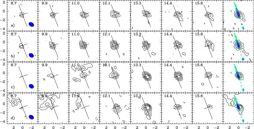
Figure 8.— SMA channel velocity images (combined data with robust 0.3) of several lines toward the position of MM1, the source from which originates the thermal radio jet. The lines are presented in the following order: row a) SO₂ 16_3,13–16_2,14, row b) SO₂ 13_2,12–13_1,13, row c) SO $5_{5}$–$4_{4}$ and row d) H₂CO 3_1,2–2_1,1. The velocity channels are 1.14 km s^-1 wide and the central velocity is indicated in the upper left corner of the channels. The disk velocity center is 13.0 km s^-1 while the dense core velocity is 11.8 km s^-1. Contours are -5, -3, 3, 5, 7, 9, 11 and 13 times the rms noise level of each image, given in Table 1. The direction of the radio jet and the direction perpendicular to it are marked by two straight lines in each channel. The last channel of each row shows the zero order moment of each line (contours) superimposed on the 3.5 cm continuum radio jet image (grey scale). The synthesized beam sizes appear as a blue ellipse in the first channel of each row. It is evident that the peak of the emission moves from east to west on the SO₂ velocity cubes.

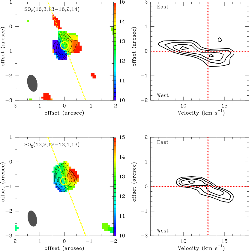
Figure 9.— SO₂ 16_3,13–16_2,14 and SO₂ 13_2,12–13_1,13 zero (contours) and first order (colour scales) moment images (left panels) toward MM1. Their corresponding position–velocity diagrams with a perpendicular crosscut through the jet axis (P.A.$=111\arcdeg$) at the position of MM1 are shown in the right–hand panels. The contour levels for the zeroth order moments are -30, 30, 50, 70 and 90% the flux peak, and the colour bar is in  km s^-1. The emission is integrated over the velocity range 7–19 km s^-1 for both lines. The yellow dotted line marks the orientation of the radio jet. The yellow circle is centered at the position of the millimeter peak continuum emission of MM1 and has the equivalent radius of the upper limit of the size obtained from the 1.4 mm millimeter image (Paper I). In the position–velocity diagrams (panels on the right) the vertical dotted line marks the disk velocity. East is at the top and west is at the bottom of both position–velocity diagrams. The contours are 50% to 95% with a step of 15% the peak flux.

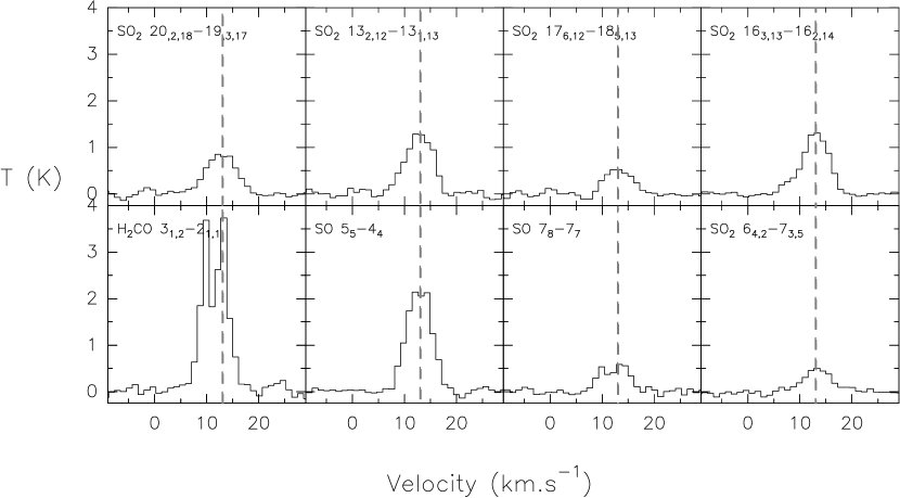
Figure 10.— Spectra of several transitions toward MM1 from low angular resolution data. The dashed line is placed at the velocity of the disk peak emission (13.0 km s^-1 on average). Intensity is in Kelvin.

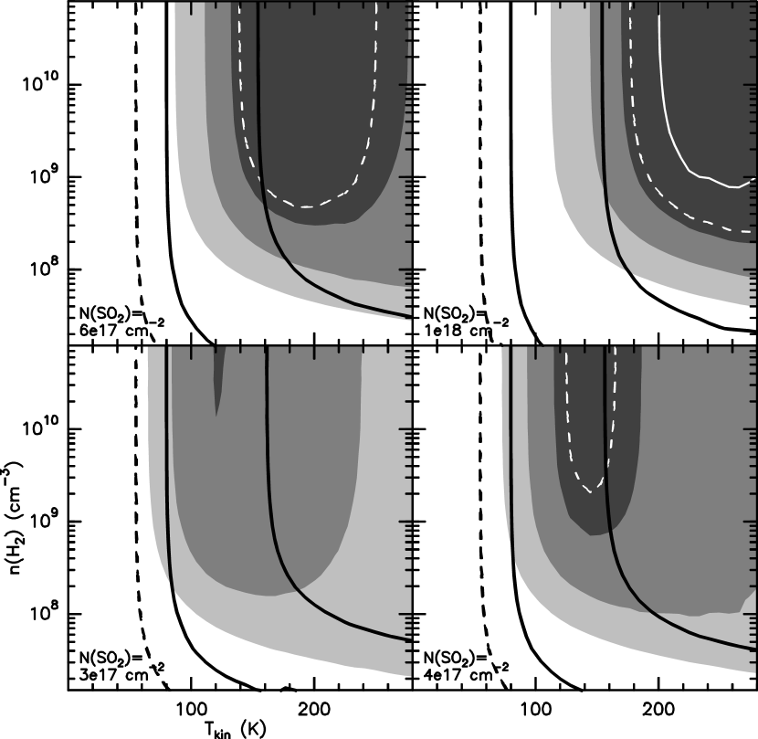
Figure 11.— Plot of the set of RADEX solutions in the $n$(H₂)-$T_{\rm kin}$ plane for the emission associated with the MM 1 disk for four different values of the SO₂ column density (from bottom-left to top-right panels): 3, 4, 6 and $10\times 10^{17}$ cm^-2. The grey image gives the values of the $\chi^{2}$ solutions for the SO₂ line ratios (see § 4.1). The increase of the grey tonalities (from lighter to darker) indicated a decrease in the $\chi^{2}$ values. The solid and dashed white contours show the 68% and 99% confidence region of the $\chi^{2}$. The dashed black line shows the range of solutions for a brightness temperature of the 13_2,12-13_1,13 line of 50 K, which is the value measured at the high angular resolution map. The area between the two black solid line shows the range of valid solutions for the 13_2,12-13_1,13 brightness temperature if the SO₂ has an emitting size between $0\farcs 5$ and $1\farcs 0$ (see § 4.1).

Table 4Size of the SO₂ disk. II. From high to low angular resolution ratio

	SO2	SO2
Parameter	132,12-131,13	163,13-162,14
$T_{\rm mb}^{\rm high}$ (K)	$50\pm 8$	$53\pm 10$
$T_{\rm mb}^{\rm low}$ (K)	$1.33\pm 0.05$	$1.32\pm 0.03$
$T_{\rm mb}^{\rm high}/T_{\rm mb}^{\rm low}$	$37.6\pm 6.2$	$40.2\pm 7.6$
$\Omega$ (arcsec)	$0\farcs 62\pm 0\farcs 10$	$0\farcs 59\pm 0\farcs 11$
$\Omega$ (AU)	$1054\pm 170$	$1003\pm 187$

In this section we estimate the physical characteristics of the MM1 disk, such as volume density and temperature by means of RADEX modeling. We used RADEX to simulate the line intensities of the five observed SO₂ transitions (Fig. 10). The RADEX code is a non-LTE molecular radiative transfer code which assumes an isothermal homogeneous medium (van der Tak et al. 2007). This assumption is reasonable as a first approach to constrain the physical properties of the gas traced by the SO₂ since the observed lines are optically thick (see below). We explored a range of values between 50 and 300 K in the kinetic temperature, between $10^{7}$ and $10^{11}$ cm^-3 in the volume density, $n$(H₂), and between $10^{14}$ and $10^{19}$ cm^-2 in the SO₂ column density, $N$(SO₂). In order to constrain the physical properties of the SO₂ emitting region the next scheme was followed:

• We first computed the $\chi^{2}$ parameter (which is a measure of how well the model fits the observations) for the line ratio of the 16_3,13-16_2,14, 17_6,12-18_5,13, 20_2,18-19_3,17 and 6_4,2-7_3,5 SO₂ transitions with respect to the 13_2,12-13_1,13 SO₂ transition. This approach assumes that all the transitions trace the same region (the images from the combined data of these lines give similar deconvolved sizes all with deconvolved major axis $\lesssim 3\arcsec$). Figure 11 shows in grey scale a set of the best solutions in the $n$(H₂)-$T_{\rm kin}$ plane for four different values of the SO₂ column density. The best set of solutions (darkest areas of Fig. 11) indicates that the SO₂ arises from hot and very dense molecular gas, as expected if it is associated with the MM1 disk. Indeed, the line ratios do not constrain well the physical values of the gas but rather yield lower limits: $n$(H₂)$\gtrsim 3\times 10^{8}$ cm^-3 and $T_{\rm kin}\gtrsim 120$ K. In addition, RADEX predicts a very large molecular column density of SO₂, $N$(SO₂)$\gtrsim 3\times 10^{17}$ cm^-2, indicating that the observed lines are optically thick.

• As an additional constraint, we take into account the possible values of the SO₂ 13_2,12-13_1,13 and 16_3,13-16_2,14 brightness temperatures. As a lower limit we can use the main beam brightness temperature measured in the highest angular resolution maps, $T_{\rm mb}=50$ K (it is shown in Figure 11 as a dashed line). However, it is not enough to further constraint the physical conditions of the gas associated with the SO₂ emission. As a further constrain, the true brightness temperature of the SO₂ can be estimated if the source size is known. The high angular resolution maps of the 13_2,12-13_1,13 and 16_3,13-16_2,14 integrated emission yield a size for the SO₂ of $\simeq 0\farcs 8$–$1\farcs 0$ (see Table 3). This size can also be independently obtained by comparing the main beam brightness temperature of the low and high angular resolution maps of these two lines. For a Gaussian distribution of the emission, the ratio of the low to high angular resolution line intensity is $T_{\rm mb}^{\rm high}/T_{\rm mb}^{\rm low}=(\theta_{\rm low}^{2}+\Omega^{2})/(\theta_{\rm high}^{2}+\Omega^{2})$, where $\Omega$ is the source size, $\theta_{\rm high}$ and $\theta_{\rm low}$ are the beam sizes of the high and low angular resolution maps, respectively. Table 4 shows the intensities of the 13_2,12-13_1,13 and 16_3,13-16_2,14 lines for the low and high angular resolution maps. Using this method, the SO₂ source size is slightly smaller, $0\farcs 6\pm 0\farcs 1$ (Table 4). Therefore, we adopt a SO₂ disk size in the range of $0\farcs 5$–$1\farcs 0$ (425–850 AU). This implies that the brightness temperatures of the 13_2,12-13_1,13 and 16_3,13-16_2,14 lines are $\simeq 62$–84 K and 68–94 K, respectively. The area within the solid lines of Figure 11 shows the possible solutions that yield an SO₂ 13_2,12-13_1,13 brightness temperature within this range.

By combining the two aforementioned criteria and using the 99% confidence interval of the $\chi^{2}$, the possible reasonable solutions get significantly reduced. Thus, for example, $N\mathrm{(SO_{2})}=1\times 10^{18}$ cm^-2 has better $\chi^{2}$ solutions than lower values of the SO₂ column density, but these solutions predict a brightness temperature significantly higher than the expected value. The best solutions are for a kinetic temperature of $T_{\rm kin}=120$–160 K and a volume density of $n\mathrm{(H_{2})}\gtrsim 2\times 10^{9}$ cm^-3. These values are, approximately, in agreement with those derived from the dust emission associated with MM1 disk (Paper I). The possible SO₂ column densities are in the 4–$6\times 10^{17}$ cm^-2 range.

The abundance of the SO₂ emission can be estimated from the derived SO₂ column density taking into account the filling factor of the observations. In Paper I, we used the 1.4 mm dust emission at an angular resolution of $\simeq 0\farcs 51$ to derive a beam averaged gas column density of $N\mathrm{(H_{2})}\simeq 1.1\times 10^{25}$ cm^-2. For this angular resolution the filling factor of a source with a $0\farcs 5$–$1\farcs 0$ size is 0.49–0.80. Therefore, the SO₂ beam averaged column density at this angular resolution is 2.0–$4.8\times 10^{17}$ cm^-2, which implies a SO₂ abundance of $X\mathrm{[SO_{2}]}\simeq 1.7$–$4.2\times 10^{-8}$.

5. DISCUSSION

5.1. A rotating molecular disk/ring toward MM1

5.1.1 Evidence for a disk

The emission of the SO₂, SO and H₂CO at the position of MM1 seems to consist of a compact rotating circumstellar structure, probably a rotating gaseous disk or ring (Figs. 8 and 9). All the species detected with the SMA toward MM1 are expected to be present in a $\sim 150$ K disk, in which a central protostar is evaporating the gas from the grain mantles (e.g., Charnley 1997; Maret et al. 2004). In addition, the SO₂ abundance (2–4$\times 10^{-8}$) obtained with RADEX is consistent with that found in the innermost parts of the envelopes of hot cores, where the temperature is greater than 100 K (van der Tak et al. 2003).

The case for a rotating disk surrounding the protostar in MM1 becomes stronger in light of the new results reported here. The velocity gradient within the molecular emission of the SO₂ lines appears compact, with a radius R$\simeq$425–850 AU, surrounding the compact (R$<150$ AU) 1.4 mm dusty disk and the thermal radio jet (Fig. 7). Furthermore, the position angle between the extreme blue and redshifted channels of two SO₂ lines (see §3.4), is roughly perpendicular to the radio jet axis, with a position angle 110–130$\arcdeg$.

5.1.2 Dynamical mass

We now estimate the dynamical mass with the 50% contour of the SO₂ 16_3,13–16_2,14 and SO₂ 13_2,12–13_1,13 position-velocity diagrams in Fig. 9. We assume an equilibrium between the centrifugal and gravitational forces and also that the disk is seen edge–on. We use the virial equation, $M_{\rm dyn}=(v^{2}R)/G$, which requires that the dominant force is due to gravity. This gives a dynamical mass of 15$\pm 5$ M_☉ and 11$\pm 3$ M_☉ (Table 3) by using the SO₂ 16_3,13–16_2,14 and the SO₂ 13_2,12–13_1,13 data. The virial approximation is valid when the system is spherically symmetric regardless of its density distribution. It is in addition a good approximation for thick disks (as appears to be the case of MM1, §5.1.3).

The continuum observations toward MM1 (Paper I) have shown a very compact disk–like structure ($R<150$ AU, 4.1 M_☉) and a more extended and weaker envelope ($R\sim 1500$ AU, 1.5 M_☉). On the other hand the SO₂ rotating structure has a radius of 425–850 AU. For this radius range the gravitational effect of the compact disk–like structure could be considered as part of the central mass, therefore, using the virial equation is a reasonable approximation to find out the protostar plus inner–disk mass.

To probe the impact of the extended molecular structure on the centrifugal balance of forces in MM1, we consider an additional term due to a flattened disk, representing the SO₂ disk–like structure. We assume that this structure has a mass of 1.5 M_☉ and a radius of 1500 AU, the characteristics of the dusty envelope of MM1. We also assume a disk surface density inversely proportional to the distance from the protostar ($\rho(R)\propto R^{-1}$). In addition, we include another term to the balance of forces due to a pressure gradient $(1/\rho)(dP/dR)$ (see Torrelles et al. 1986). To estimate this pressure term we use either a sound speed of 0.7 km s^-1 (corresponding to a 150 K gas temperature), or a turbulent plus thermal random velocity of $\sim 1$ km s^-1. Both terms (extended disk and pressure gradient) could induce a departure from the Keplerian behavior of the disk. However, we find that both are one order of magnitude smaller than that of the central mass. Thereby, the central mass obtained is essentially the same as that estimated with the virial approximation.

If the SO₂ rotating structure is not edge–on (i.e., i$\neq 90\arcdeg$), the derived total mass is just a lower limit. Nevertheless, the edge–on approximation seems adequate for the MM1 disk, as the thermal radio jet is one of the largest jets ($\sim 5.3$ pc in projected distance) observed up to now. Therefore, it is expected to be close to the plane of the sky (Martí et al. 1993). However, Yamashita et al. (1987) estimated an inclination between 60$\arcdeg$ and 74$\arcdeg$ by modeling the geometry of the infrared reflection nebula, which would increase the dynamical mass to a range of 14–20 M_☉.

5.1.3 Stability of the disk

Due to the high mass of the compact dusty disk (about 4 M_☉), it is reasonable to ask whether the molecular disk is stable against gravitational disturbances. If we take as the disk parameters T$=120$–160 K, N$=1\times 10^{25}$ cm^-2 (and hence the surface density, $\Sigma=N\cdot\mu\cdot\mathrm{m_{H}}=40$ g cm^-2, using a mean molecular weight of 2.3 for molecular hydrogen and helium at 10 K), and the disk velocity 3.4–4.3 km s^-1 at 876–740 AU (Table 3) from the center of the disk, we can approximate the value of the Toomre parameter (Toomre 1964), defined as

$$Q=\frac{\mathrm{c_{s}}\cdot\kappa}{\pi\cdot G\cdot\Sigma}\quad.$$

In the equation above, $\mathrm{c_{s}}$ is the sound velocity, $\kappa$ is the epicyclic frequency (which can be approximated as $\Omega$ for Keplerian motion or as $2\Omega$ for solid body rotation, $\Omega$ being the angular velocity), G is the gravitational constant and $\Sigma$ is the surface density. If Q is less than 1 then the disk is unstable. First, we estimate the Toomre parameter using the thin disk assumption (e.g., Kratter & Matzner 2006), and a high epicyclic frequency (that of solid body rotation). The resulting value is $Q=0.42$–0.72. It appears that the molecular disk would be unstable even in the unlikely case of a rigid body rotation.

However, Cesaroni et al. (2007) (see also Durisen et al. 2001) pointed out that the thickness of disks should have a great stabilizing effect on these. Following their approximation for thick disks by assuming a disk thickness H$=\mathrm{c_{s}^{2}}/(\pi G\Sigma)=35$–47 AU, a disk mass of $\mathrm{M_{d}}=4$ M_☉, and a total mass in a wide range of $\mathrm{M_{tot}}=10$–20 M_☉, we obtain Q$=\sqrt{2\cdot(\mathrm{H/R})\cdot(\mathrm{M_{tot}}/\mathrm{M_{d}}})=0.40$–0.80, which is again smaller than unity.

Although the Q$=0.8$ case is closer to unity, the MM1 disk–like structure seems therefore probably unstable. In such a case, the gravitational perturbations can lead to the appearance of dense spiral arms, rings, arcuate structures or even dense fragments, which could result in the formation of a clumpy structure (Durisen et al. 2001, 2007).

5.1.4 Mass of the protostar

We can also roughly estimate the mass of the protostar at the position of MM1. If we assume an edge–on disk (which provides again with a lower limit), since the gas plus dust mass of the MM1 disk was estimated from the 1.4 mm millimeter continuum emission (see Paper I) to be about 4$\pm$1 M_☉, the mass of the protostar would be about 7$\pm$4–11$\pm$6 M_☉. Although the estimation has an uncertainty larger than a 50%, this agrees well with the expected mass for a $>3300$ L_☉ (Paper I) protostar, which could be related to a $\sim 10$ M_☉ ZAMS star (Table 5 of Molinari et al. 1998).

5.1.5 Absorption of disk emission by a foreground cloud

The blueshifted emission of the SO $5_{5}$–$4_{4}$ and H₂CO 3_1,2–2_1,1 lines from the disk appears to be missing (Fig. 8). One possibility is that the interferometer has filtered out some extended flux. However one would expect some remnant emission from the rotating structure. Another possibility is that gas from the foreground component of the cloud between 8.5 and 11.8 km s^-1 (Figs. 3 and 6) may have absorbed the blueshifted emission from the disk. Firstly, the extended dense molecular component traced by the C¹⁷O and H₂CO appears blueshifted at the same velocity range where the missing velocity disk component is observed in SO $5_{5}$–$4_{4}$ and H₂CO 3_1,2–2_1,1. And secondly, the other SO transition, SO $7_{8}$–$7_{7}$, shows only compact emission toward MM1, as in the other SO₂ lines. This SO line and also the SO₂ lines, have a higher excitation, therefore they can only be excited in the hot environment around the disk.

5.2. Emission from the cavity walls

Figs. 2 and 3 show the SO emission extending about $10\arcsec$–$15\arcsec$ to the north of the position of MM1. The SO emission appears clumpy, with some of the clumps probably associated with the molecular outflows of the region. In particular, the SO $5_{5}$–$4_{4}$ line emission, and also in a lesser measure the H₂CO, seems also to surround the thermal radio jet axis, with a geometry reminiscent of a V-shape. A possibility is that part of the emission of these lines is tracing the walls of the outflow cavity excavated by the thermal radio jet originated at the position of MM1 (as that of outflow cavities associated with low-mass protostars; see e.g., Lee et al. 2000; Arce & Sargent 2006; Jørgensen et al. 2007; Santiago-García et al. 2009). This quiescent molecular emission (i.e., showing narrow lines) associated with powerful outflows could be photoilluminated by the UV radiation generated in the shocks within the outflows, as has been observed in several HH objects (Girart et al. 2002, 2005; Viti et al. 2003, 2006). Indeed, in the case of the HH 80–81 and HH 80N system, there is a shock–induced photodissociation region along all the thermal radio jet, reported by Molinari et al. (2001).

5.3. Is the Molecular Core actually a hot core?

The only molecular lines clearly detected toward the molecular core (MC) northwest of MM2 are SO $5_{5}$–$4_{4}$ and H₂CO 3_1,2–2_1,1. This source has been previously identified as a hot molecular core (Qiu & Zhang 2009). Both lines show a narrow component (e.g., the FWHM of the SO line is $\sim 2.5$ km s^-1) centered at  $v_{\rm LSR}$ $\simeq$10–12 km s^-1, and a redshifted wing spreading up to about 30 km s^-1. The narrower component is related to the quiescent gas in the molecular core, while the component with the wider velocity range is probably due to shocked gas entrained by the outflows of the region. Herein, we discuss the possible origin of the MC.

It has been proposed that the MC is a hot core surrounding a massive protostar. This is based on the detection of hot core molecular tracers, such as CH₃OH, HNCO, and OCS (Qiu & Zhang, 2009). However, we note that the temperature estimated in the MC is $\simeq 45$ K (Qiu & Zhang, 2009) which is about a factor of 2 lower than the temperature found in hot cores. In addition, the lack of dust emission associated with the MC ($\lesssim 10$ mJy at 1.4 mm) implies that for the aforementioned temperature the total mass of the MC has an upper limit of $\sim 0.25$ M_☉ (Qiu & Zhang, 2009), too small for a hot core. Could it be possible that MC is a hot corino such as IRAS 16293–2422 (Rao et al., 2009)? At the distance of IRAS 18162–2048, IRAS 16293–2422 source B would have a flux density of 10 mJy at 1.4 mm, below the upper limit of our observations. But, the MC temperature is still lower than that of this hot corino and the intensity of the observed molecular lines in source IRAS 16293–2422 B would be far from being detected with the current sensitivity at the distance of IRAS 18162–2048.

A possible alternative is that MC is tracing the interaction of the dense molecular core with a strong shock produced in a molecular outflow in a way that the external heating and the radiation of the gas produced a strong outgassing phase (Viti et al. 2006), exciting many molecular transitions, as it has been observed in other sources, such as Orion (Liu et al. 2002; Zapata et al. 2010; see also Chernin & Wright 1996).

There is a class I CH₃OH maser (Kurtz et al. 2004; Qiu & Zhang 2009) detected about $1\arcsec$ south–east of MC. This class of masers is associated with shocked molecular gas (Kurtz et al. 2004). The most likely scenario is that the molecular outflow from MM2 has encountered a molecular core at the MC position. The northwest lobe of this outflow is redshifted and its path is crossed by the MC (see Figs. 3 and 6). Therefore, it seems possible that the outflow could partially hit the molecular core at MC, producing a stationary bow shock which could entrain the molecular gas, as found in some molecular outflows such as L1157 and IRAS 04166+2706 (Zhang et al. 1995; Santiago-García et al. 2009; Tafalla et al. 2010). Given the location of the MC, it is also possible that it is not an isolated core, but it forms part of the cavity walls associated with the thermal radio jet (section §5.2).

6. CONCLUSIONS

We have performed an SMA observational study of the molecular gas toward the central region of IRAS 18162–2048, and have obtained the following main results.

• The SO₂ 16_3,13–16_2,14 and SO₂ 13_2,12–13_1,13 data show a compact (R$\simeq 425$–850 AU) molecular disk–like structure spatially coincident with the position of the compact millimeter dusty source MM1 and the radio jet located at the IRAS 18162–2048 position. The molecular structure is perpendicular to the radio jet axis and it shows a clear velocity gradient that we interpret as rotation. The dynamical mass (11–15 M_☉) allowed us to derive the mass of the protostar (7–11 M_☉), making use of the mass that was inferred from the continuum data (Paper I).

  The RADEX analysis constrains the disk–like structure temperature between 120 and 160 K and its volume density as $\gtrsim 2\times 10^{9}$ cm^-3. We have also found that the rotating system could be unstable due to gravitational disturbances.

• The C¹⁷O 2–1 emission shows an elongated structure of about 0.2 pc $\times$ 0.1 pc with an orientation roughly perpendicular to the radio jet. This emission seems to belong to the dense core in which the protostars associated with the MM1, MM2 and MC sources are forming.

• The H₂CO and the SO emission appears clumpy and is mainly enhanced toward the position of MM1 and MC. It is possibly tracing in part the cavity walls excavated by the thermal radio jet. At the position of MC, it shows a line profile with a red wing extending up to tens of  km s^-1. This line profile is probably due to shocked gas entrained by the outflows in the region. We speculate that a possible scenario is the interaction between the outflow associated with MM2 and the dense molecular core at this position.

References

- Andrè et al. (1993) Andrè, P., Ward-Thompson, D., & Barsony, M. 1993, ApJ, 406, 122
- Arce & Sargent (2006) Arce, H. G. & Sargent, A. I. 2006, ApJ, 646, 1070
- Arce et al. (2007) Arce, H. G., Shepherd, D., Gueth, F., Lee, C., Bachiller, R., Rosen, A., & Beuther, H. 2007, Protostars and Planets V, 245
- Aspin & Geballe (1992) Aspin, C. & Geballe, T. R. 1992, A&A, 266, 219
- Banerjee & Pudritz (2007) Banerjee, R. & Pudritz, R. E. 2007, ApJ, 660, 479
- Baumgardt & Klessen (2011) Baumgardt, H. & Klessen, R. S. 2011, MNRAS, 321
- Beech & Mitalas (1994) Beech, M. & Mitalas, R. 1994, ApJS, 95, 517
- Benedettini et al. (2004) Benedettini, M., Molinari, S., Testi, L., & Noriega-Crespo, A. 2004, MNRAS, 347, 295
- Beuther & Walsh (2008) Beuther, H. & Walsh, A. J. 2008, ApJ, 673, L55
- Bonnell et al. (1998) Bonnell, I. A., Bate, M. R., & Zinnecker, H. 1998, MNRAS, 298, 93
- Cantó et al. (2009) Cantó, J., Curiel, S., & Martínez-Gómez, E. 2009, A&A, 501, 1259
- Carrasco-González et al. (2010) Carrasco-González, C., Rodríguez, L. F., Anglada, G., Martí, J., Torrelles, J. M., & Osorio, M. 2010, Science, 330, 1209
- Cesaroni (2005) Cesaroni, R. 2005, in IAU Symposium, Vol. 227, Massive Star Birth: A Crossroads of Astrophysics, ed. R. Cesaroni, M. Felli, E. Churchwell, & M. Walmsley, 59–69
- Cesaroni et al. (2007) Cesaroni, R., Galli, D., Lodato, G., Walmsley, C. M., & Zhang, Q. 2007, Protostars and Planets V, 197
- Charnley (1997) Charnley, S. B. 1997, ApJ, 481, 396
- Chernin & Wright (1996) Chernin, L. M. & Wright, M. C. H. 1996, ApJ, 467, 676
- Clarke & Bonnell (2008) Clarke, C. J. & Bonnell, I. A. 2008, MNRAS, 388, 1171
- Cunningham et al. (2009) Cunningham, N. J., Moeckel, N., & Bally, J. 2009, ApJ, 692, 943
- Curiel et al. (2006) Curiel, S., Ho, P. T. P., Patel, N. A., Torrelles, J. M., Rodríguez, L. F., Trinidad, M. A., Cantó, J., Hernández, L., Gómez, J. F., Garay, G., & Anglada, G. 2006, ApJ, 638, 878
- Durisen et al. (2007) Durisen, R. H., Boss, A. P., Mayer, L., Nelson, A. F., Quinn, T., & Rice, W. K. M. 2007, Protostars and Planets V, 607
- Durisen et al. (2001) Durisen, R. H., Mejia, A. C., Pickett, B. K., & Hartquist, T. W. 2001, ApJ, 563, L157
- Fernández-López et al. (2011) Fernández-López, M., Curiel, S., Girart, J. M., Ho, P. T. P., Patel, N., & Gómez, Y. 2011, AJ, 141, 72
- Franco-Hernández et al. (2009) Franco-Hernández, R., Moran, J. M., Rodríguez, L. F., & Garay, G. 2009, ApJ, 701, 974
- Frau et al. (2010) Frau, P., Girart, J. M., Beltrán, M. T., Morata, O., Masqué, J. M., Busquet, G., Alves, F. O., Sánchez-Monge, Á., Estalella, R., & Franco, G. A. P. 2010, ApJ, 723, 1665
- Frerking et al. (1982) Frerking, M. A., Langer, W. D., & Wilson, R. W. 1982, ApJ, 262, 590
- Galván-Madrid et al. (2010) Galván-Madrid, R., Zhang, Q., Keto, E., Ho, P. T. P., Zapata, L. A., Rodríguez, L. F., Pineda, J. E., & Vázquez-Semadeni, E. 2010, ApJ, 725, 17
- Girart et al. (2006) Girart, J. M., Rao, R., & Marrone, D. P. 2006, Science, 313, 812
- Girart et al. (1994) Girart, J. M., Rodríguez, L. F., Anglada, G., Estalella, R., Torrelles, J. M., Martí, J., Pena, M., Ayala, S., Curiel, S., & Noriega-Crespo, A. 1994, ApJ, 435, L145
- Girart et al. (2005) Girart, J. M., Viti, S., Estalella, R., & Williams, D. A. 2005, A&A, 439, 601
- Girart et al. (2002) Girart, J. M., Viti, S., Williams, D. A., Estalella, R., & Ho, P. T. P. 2002, A&A, 388, 1004
- Gómez et al. (2003) Gómez, Y., Rodríguez, L. F., Girart, J. M., Garay, G., & Martí, J. 2003, ApJ, 597, 414
- Hatchell et al. (1998) Hatchell, J., Thompson, M. A., Millar, T. J., & MacDonald, G. H. 1998, A&A, 338, 713
- Ho et al. (2004) Ho, P. T. P., Moran, J. M., & Lo, K. Y. 2004, ApJ, 616, L1
- Jijina & Adams (1996) Jijina, J. & Adams, F. C. 1996, ApJ, 462, 874
- Jiménez-Serra et al. (2007) Jiménez-Serra, I., Martín-Pintado, J., Rodríguez-Franco, A., Chandler, C., Comito, C., & Schilke, P. 2007, ApJ, 661, L187
- Jørgensen et al. (2007) Jørgensen, J. K., Bourke, T. L., Myers, P. C., Di Francesco, J., van Dishoeck, E. F., Lee, C., Ohashi, N., Schöier, F. L., Takakuwa, S., Wilner, D. J., & Zhang, Q. 2007, ApJ, 659, 479
- Kahn (1974) Kahn, F. D. 1974, A&A, 37, 149
- Keto (2002) Keto, E. 2002, ApJ, 568, 754
- Keto & Wood (2006) Keto, E. & Wood, K. 2006, ApJ, 637, 850
- Klaassen et al. (2009) Klaassen, P. D., Wilson, C. D., Keto, E. R., & Zhang, Q. 2009, ApJ, 703, 1308
- Kratter & Matzner (2006) Kratter, K. M. & Matzner, C. D. 2006, MNRAS, 373, 1563
- Krumholz et al. (2005) Krumholz, M. R., Klein, R. I., & McKee, C. F. 2005, in Protostars and Planets V, 8271
- Kurtz et al. (2004) Kurtz, S., Hofner, P., & Álvarez, C. V. 2004, ApJS, 155, 149
- Larson & Starrfield (1971) Larson, R. B. & Starrfield, S. 1971, A&A, 13, 190
- Lee et al. (2000) Lee, C., Mundy, L. G., Reipurth, B., Ostriker, E. C., & Stone, J. M. 2000, ApJ, 542, 925
- Liu et al. (2002) Liu, S., Girart, J. M., Remijan, A., & Snyder, L. E. 2002, ApJ, 576, 255
- Maret et al. (2004) Maret, S., Ceccarelli, C., Caux, E., Tielens, A. G. G. M., Jørgensen, J. K., van Dishoeck, E., Bacmann, A., Castets, A., Lefloch, B., Loinard, L., Parise, B., & Schöier, F. L. 2004, A&A, 416, 577
- Martí et al. (1993) Martí, J., Rodríguez, L. F., & Reipurth, B. 1993, ApJ, 416, 208
- Martí et al. (1995) —. 1995, ApJ, 449, 184
- Martí et al. (1998) —. 1998, ApJ, 502, 337
- Martí et al. (1999) Martí, J., Rodríguez, L. F., & Torrelles, J. M. 1999, A&A, 345, L5
- Martín-Pintado et al. (2005) Martín-Pintado, J., Jiménez-Serra, I., Rodríguez-Franco, A., Martín, S., & Thum, C. 2005, ApJ, 628, L61
- McKee & Tan (2003) McKee, C. F. & Tan, J. C. 2003, ApJ, 585, 850
- Moeckel & Clarke (2011) Moeckel, N. & Clarke, C. J. 2011, MNRAS, 410, 2799
- Molinari et al. (1998) Molinari, S., Brand, J., Cesaroni, R., Palla, F., & Palumbo, G. G. C. 1998, A&A, 336, 339
- Molinari et al. (2001) Molinari, S., Noriega-Crespo, A., & Spinoglio, L. 2001, ApJ, 547, 292
- Nakano (1989) Nakano, T. 1989, ApJ, 345, 464
- Norberg & Maeder (2000) Norberg, P. & Maeder, A. 2000, A&A, 359, 1025
- Patel et al. (2005) Patel, N. A., Curiel, S., Sridharan, T. K., Zhang, Q., Hunter, T. R., Ho, P. T. P., Torrelles, J. M., Moran, J. M., Gómez, J. F., & Anglada, G. 2005, Nature, 437, 109
- Qiu & Zhang (2009) Qiu, K. & Zhang, Q. 2009, ApJ, 702, L66
- Rao et al. (2009) Rao, R., Girart, J. M., Marrone, D. P., Lai, S., & Schnee, S. 2009, ApJ, 707, 921
- Reipurth & Graham (1988) Reipurth, B. & Graham, J. A. 1988, A&A, 202, 219
- Rodríguez et al. (2008) Rodríguez, L. F., Moran, J. M., Franco-Hernández, R., Garay, G., Brooks, K. J., & Mardones, D. 2008, AJ, 135, 2370
- Santiago-García et al. (2009) Santiago-García, J., Tafalla, M., Johnstone, D., & Bachiller, R. 2009, A&A, 495, 169
- Sault et al. (1995) Sault, R. J., Teuben, P. J., & Wright, M. C. H. 1995, in Astronomical Society of the Pacific Conference Series, Vol. 77, Astronomical Data Analysis Software and Systems IV, ed. R. A. Shaw, H. E. Payne, & J. J. E. Hayes, 433
- Stecklum et al. (1997) Stecklum, B., Feldt, M., Richichi, A., Calamai, G., & Lagage, P. O. 1997, ApJ, 479, 339
- Tafalla et al. (2010) Tafalla, M., Santiago-García, J., Hacar, A., & Bachiller, R. 2010, A&A, 522, A91
- Toomre (1964) Toomre, A. 1964, ApJ, 139, 1217
- Torrelles et al. (1986) Torrelles, J. M., Ho, P. T. P., Rodriguez, L. F., & Canto, J. 1986, ApJ, 305, 721
- Trinidad et al. (2006) Trinidad, M. A., Curiel, S., Torrelles, J. M., Rodríguez, L. F., Migenes, V., & Patel, N. 2006, AJ, 132, 1918
- van der Tak et al. (2007) van der Tak, F. F. S., Black, J. H., Schöier, F. L., Jansen, D. J., & van Dishoeck, E. F. 2007, A&A, 468, 627
- van der Tak et al. (2003) van der Tak, F. F. S., Boonman, A. M. S., Braakman, R., & van Dishoeck, E. F. 2003, A&A, 412, 133
- van der Tak et al. (2006) van der Tak, F. F. S., Walmsley, C. M., Herpin, F., & Ceccarelli, C. 2006, A&A, 447, 1011
- Viti et al. (2003) Viti, S., Girart, J. M., Garrod, R., Williams, D. A., & Estalella, R. 2003, A&A, 399, 187
- Viti et al. (2006) Viti, S., Girart, J. M., & Hatchell, J. 2006, A&A, 449, 1089
- Walmsley (1995) Walmsley, M. 1995, in Revista Mexicana de Astronomia y Astrofisica, vol. 27, Vol. 1, Revista Mexicana de Astronomia y Astrofisica Conference Series, ed. S. Lizano & J. M. Torrelles, 137
- Wolfire & Cassinelli (1987) Wolfire, M. G. & Cassinelli, J. P. 1987, ApJ, 319, 850
- Yamashita et al. (1991) Yamashita, T., Murata, Y., Kawabe, R., Kaifu, N., & Tamura, M. 1991, ApJ, 373, 560
- Yamashita et al. (1987) Yamashita, T., Sato, S., Nagata, T., Suzuki, H., Hough, J. H., McLean, I. S., Garden, R., & Gatley, I. 1987, A&A, 177, 258
- Yamashita et al. (1989) Yamashita, T., Suzuki, H., Kaifu, N., Tamura, M., Mountain, C. M., & Moore, T. J. T. 1989, ApJ, 347, 894
- Yorke & Kruegel (1977) Yorke, H. W. & Kruegel, E. 1977, A&A, 54, 183
- Yorke & Sonnhalter (2002) Yorke, H. W. & Sonnhalter, C. 2002, ApJ, 569, 846
- Zapata et al. (2009) Zapata, L. A., Ho, P. T. P., Schilke, P., Rodríguez, L. F., Menten, K., Palau, A., & Garrod, R. T. 2009, ApJ, 698, 1422
- Zapata et al. (2008) Zapata, L. A., Palau, A., Ho, P. T. P., Schilke, P., Garrod, R. T., Rodríguez, L. F., & Menten, K. 2008, A&A, 479, L25
- Zapata et al. (2010) Zapata, L. A., Schmid-Burgk, J., & Menten, K. M. 2010, ArXiv e-prints
- Zhang (2005) Zhang, Q. 2005, in IAU Symposium, Vol. 227, Massive Star Birth: A Crossroads of Astrophysics, ed. R. Cesaroni, M. Felli, E. Churchwell, & M. Walmsley, 135–144
- Zhang et al. (1995) Zhang, Q., Ho, P. T. P., Wright, M. C. H., & Wilner, D. J. 1995, ApJ, 451, L71
- Zinnecker & Yorke (2007) Zinnecker, H. & Yorke, H. W. 2007, ARA&A, 45, 481