Convergence of Weighted Min-Sum Decoding Via Dynamic Programming on Trees

Abstract

Applying the max-product (and belief-propagation) algorithms to loopy graphs is now quite popular for best assignment problems. This is largely due to their low computational complexity and impressive performance in practice. Still, there is no general understanding of the conditions required for convergence and/or the optimality of converged solutions. This paper presents an analysis of both attenuated max-product (AMP) decoding and weighted min-sum (WMS) decoding for LDPC codes which guarantees convergence to a fixed point when a weight parameter, $\beta$, is sufficiently small. It also shows that, if the fixed point satisfies some consistency conditions, then it must be both the linear-programming (LP) and maximum-likelihood (ML) solution.

For $(d_{v},d_{c})$-regular LDPC codes, the weight must satisfy $\beta(d_{v}-1)\leq 1$ whereas the results proposed by Koetter and Frey require instead that $\beta(d_{v}-1)(d_{c}-1)<1$. A counterexample which shows a fixed point might not be the ML solution if $\beta(d_{v}-1)>1$ is also given. Finally, connections are explored with recent work by Arora et al. on the threshold of LP decoding.

I Introduction

The introduction of turbo codes in 1993 started a revolution in coding and inference that continued with the rediscovery of low-density parity-check (LDPC) codes and culminated in optimized LDPC codes that essentially achieve the capacity of practical channels [1, 2, 3, 4]. During this time, Wiberg et al. advanced the analysis of iterative decoding by proving a number of results for the min-sum (a.k.a. max-product) decoding algorithm [5, 6, 7]. Richardson and Urbanke also introduced the technique of density evolution (DE) to compute noise thresholds of message-passing decoding algorithms for turbo and LDPC codes [8].

For a particular noise realization, the optimality of iterative decoding solutions has also been considered by a number of authors. Weiss and Freeman have shown that the max-product (MP) assignment is locally optimal w.r.t. all single-loop and tree perturbations [9]. Unfortunately, this result is typically uninformative for LDPC codes with variables degrees larger than 2. Frey and Koetter have also shown that, with proper weights and adjustments, the attenuated max-product (AMP) decoding for LDPC codes returns the maximum-likelihood (ML) codeword if it converges to a codeword [7]. For general graphs, Wainwright et al. proposed the tree-reweighted max-product (TRMP) message-passing algorithm for computing the MAP assignment on the strictly positive Markov random field [10]. They have shown that, under some optimality conditions, the converged solution gives the MAP configuration for the graph. Their algorithm, though strictly different, has some similarity to the AMP algorithm in [7].

The linear programming (LP) decoding for LDPC codes, proposed by Feldman et al., solves a relaxed version of the ML decoding problem [11]. Since its introduction, a number of authors have looked for connections to the MP iterative decoding algorithm [12]. One interesting open question is, “What is the noise threshold of LP decoding?”. The first threshold bound for LP decoding was proposed in [13]. Using expander graph arguments, they showed that LP decoding of a rate-$\frac{1}{2}$ regular LDPC code can correct all error patterns with weight less than $0.000175$ of the block length. Since this is a worst-case analysis, the large gap to the empirical observations is not too surprising. Daskalakis et al. [14] were able to improve the threshold to $0.002$ using probabilistic arguments based on a construction of a LP dual feasible solution. In [15], Koetter and Vontobel applied girth-based arguments to the dual LP problem. For a $(3,6)$-regular LDPC code, they proved that LP decoding can tolerate a crossover probability of $p=0.01$ on the binary symmetric channel (BSC) and a noise level of $\sigma=0.5574$ on the binary-input additive white Gaussian noise channel (BIAWGNC).

Arora et al. showed recently that, for a $(3,6)$-regular LDPC code, LP decoding can tolerate a crossover probability $p=0.05$ on the BSC [16]. Instead of using a dual LP solution, they investigated the primal solution of the LP problem and proposed a local optimality condition for codewords. They proved that the local optimality implies both global optimality and LP optimality. So the probability that LP decoding succeeds is lower bounded by the probability that the correct codeword satisfies a set of local optimality conditions. Since their local optimality conditions are amenable to analysis on tree-like neighborhoods, they perform a DE analysis to obtain BSC noise thresholds for LP decoding. Using DE for memoryless binary-input output symmetric (MBIOS) channels, Halabi et al. showed that LP decoding can achieve a noise threshold $\sigma=0.735$ on the BIAWGNC [17].

The results in this paper can be seen as an extension of the work by Frey and Koetter that provides new insight into results of [15, 16]. We view both AMP and WMS [18] algorithms as computing the dynamic-programming (DP) solution to the optimal discounted-reward problem on a set of overlapping trees. This allows us to show that, for any received vector, the one-step update of the algorithm is a contraction on the space of message values when weight parameter is sufficiently small. From this, we deduce that the messages converge to a unique fixed point. We first show that, for $(d_{v},d_{c})$-regular LDPC codes, if the resulting fixed point satisfies some consistency conditions, then it must also be the LP optimum solution and, hence, the ML solution. Then, the WMS algorithm on $(d_{v},d_{c})$-regular LDPC codes with messages diverging to $\pm\infty$ is considered. We show that, for the weight $\beta=\frac{1}{d_{v}-1}$, if the WMS messages diverge to $\pm\infty$ and satisfies the consistency conditions, the corresponding hard decisions also return the ML solution.

The rest of the paper is organized as follows. Section II provides the background on factor graphs as well as the update rules of the AMP algorithm and the WMS algorithm. In Section III, we first investigate the convergence property of both algorithms, and introduce the consistency conditions for both algorithms. Then, the optimality of the hard decisions corresponding to the consistent fixed point is discussed. In Section IV, the optimality of the codeword returned by the WMS algorithm when the messages are not converged is analyzed. A conjecture about the connections between noise thresholds of the WMS decoding and noise thresholds of the LP decoding is proposed in the same section. Numerical results are described and discussed in Section V. Finally, conclusions and extensions are given in Section VI.

II Background

II-A Factor Graphs

An LDPC code can be defined by a bipartite graph $\mathcal{G}=\left(\mathcal{V},\mathcal{E}\right)$, where $\mathcal{E}$ is the set of edges, and $\mathcal{V}=\mathcal{V}_{L}\cup\mathcal{V}_{R}$ consists of variable nodes (or bit nodes) $\mathcal{V}_{L}$ and check nodes (or constraint nodes) $\mathcal{V}_{R}$. In this paper, $(d_{v},d_{c})$-regular LDPC codes are considered. That is, each variable node in $\mathcal{V}_{L}$ has $d_{v}$ edges attached to it, and each check node in $\mathcal{V}_{R}$ has $d_{c}$ edges attached to it. For a set $\mathcal{S}$, let $|\mathcal{S}|$ denote the cardinality of $\mathcal{S}$. The number of variable nodes denoted by $n$ is $|\mathcal{V}_{L}|$. Any binary vector $\boldsymbol{x}\in\{0,1\}^{n}$ is a codeword, or a valid assignment, if and only if it satisfies all check nodes in $\mathcal{V}_{R}$. We use $\mathcal{C}$ to denote the collection of all codewords. Let $\mathcal{T}_{i}^{L}$ be a computation tree of $\mathcal{G}$ which has depth $L$ and is rooted at node $i$. The set of vertices in the $\ell$th level of $\mathcal{T}_{i}^{L}$, where $\ell\leq L$, is denoted by $N(i,\ell)$. We also consider computation trees of $\mathcal{G}$ rooted at a directed edge $i\rightarrow j$ or $i\leftarrow j$ with $(i,j)\in\mathcal{E}$. For a graph $\mathcal{G}$, the size of the smallest cycle in $\mathcal{G}$ is denoted by girth($\mathcal{G}$). For a node $i\in\mathcal{V}$, we use $N(i)$ to denote the set of neighbors of $i$.

II-B Discounted Dynamic Programming on a Tree

Suppose that the computation tree $\mathcal{T}_{i}^{2L}$ has depth $2L<\frac{1}{2}\mbox{girth}(\mathcal{G})$. Then, each node in $\mathcal{T}_{i}^{2L}$ is associated with a different node in $\mathcal{G}$. Let $\mathcal{I}\subset\mathcal{V}_{L}$ be the subset of variable nodes in $\mathcal{T}_{i}^{2L}$. A binary vector $\boldsymbol{w}\in\{0,1\}^{n}$ is a valid assignment on $\mathcal{T}_{i}^{2L}$ if $\boldsymbol{w}$ satisfies all check nodes in $\mathcal{T}_{i}^{2L}$. Let $\mathcal{C}_{\mathcal{T}_{i}^{2L}}$ be the set of all valid assignments on $\mathcal{T}_{i}^{2L}$, and let $\mathcal{C}_{\mathcal{T}_{i}^{2L}}(x)\triangleq\{\boldsymbol{w}\in\mathcal{C}_{\mathcal{T}_{i}^{2L}}:w_{i}=x,w_{m}=0,\forall m\notin\mathcal{T}_{i}^{2L}\}$ be a subset of $\mathcal{C}_{\mathcal{T}_{i}^{2L}}$, where the assignment of the node $m\in\mathcal{V}_{L}\setminus\mathcal{I}$ is $0$ and the assignment of the root node is $x$. In the remainder of this paper, we often simplify $\mathcal{C}_{\mathcal{T}_{i}^{2L}}$ to $\mathcal{C}_{\mathcal{T}}$ when $i$ and $L$ are evident from the context. Similarly, we also simplify $\mathcal{C}_{\mathcal{T}_{i}^{2L}}(x)$ to $\mathcal{C}_{\mathcal{T}}(x)$.

Let $\gamma_{i}(x_{i})\triangleq\log(p_{Y|X}(y_{i}|x_{i}))$ be the log-likelihood of receiving $y_{i}\in\mathbb{R}$ given that $x_{i}\in\{0,1\}$ is transmitted at the $i$th bit. We consider the problem of finding the best assignment $\boldsymbol{w}^{*}\in\{\mathcal{C_{T}}(0)\cup\mathcal{C_{T}}(1)\}$ to a tree $\mathcal{T}_{i}^{2L}$ defined by

$$\boldsymbol{w}^{*} \triangleq\operatorname*{arg\,max}_{\boldsymbol{w}\in\{\mathcal{C_{T}}(0)\,\cup\,\mathcal{C_{T}}(1)\}}\sum_{m\in\mathcal{I}}\beta_{m}\gamma_{m}(w_{m}),$$ (1)

where $\beta_{m}=\beta^{\ell}$ if $m\in N(i,2\ell)$ and $0$ otherwise. Since $\mathcal{C_{T}}(0)$ and $\mathcal{C_{T}}(1)$ are disjoint, (1) can be separated into two subproblems. For $x\in\{0,1\}$, we first define a vector

$$\boldsymbol{w}^{*}(x)\triangleq\operatorname*{arg\,max}_{\boldsymbol{w}\in\mathcal{C_{T}}(x)}\sum_{m\in\mathcal{I}}\beta_{m}\gamma_{m}(w_{m}),$$ (2)

and a function

$$\mu_{i}(x) \triangleq\max_{\boldsymbol{w}\in\mathcal{C_{T}}(x)}\sum_{m\in\mathcal{I}}\beta_{m}\gamma_{m}(w_{m}),$$ (3)

where $\mu_{i}(x)$ is the optimal reward for assigning $x$ to the root node of $\mathcal{T}_{i}^{2L}$, and $\boldsymbol{w}^{*}(x)$ is the corresponding best assignment. Then, the solution of (1) is obtained by choosing $\boldsymbol{w}^{*}(x^{*})$ where $x^{*}=\operatorname*{arg\,max}_{x\in\{0,1\}}\mu_{i}(x)$. Note that $\mu_{i}(\cdot)$ is only a function of the assignment to the root node of $\mathcal{T}_{i}^{2L}$. Therefore, finding the best assignment of the tree $\mathcal{T}_{i}^{2L}$ is equivalent to finding the best assignment of the root node of $\mathcal{T}_{i}^{2L}$.

The RHS in (3) can be rewritten as

$$\mu_{i}(x) =\gamma_{i}(x)+\max_{\boldsymbol{w}\in\mathcal{C}_{\mathcal{T}}(x)}\sum_{\ell=1}^{L}\sum_{m\in N(i,2\ell)}\beta^{\ell}\gamma_{m}(w_{m}).$$ (4)

This suggests that we can compute $\mu_{i}(x)$ recursively by using DP. In the $(\ell+1)$th iteration, we compute the optimal discounted total reward $\mu_{i\rightarrow j}^{(\ell+1)}(x)$ of assigning $x$ to the directed edge $i\rightarrow j$ by

$$\mu_{i\rightarrow j}^{(\ell+1)}(x) =\gamma_{i}(x)+\beta\sum_{k\in N(i)\backslash j}\mu_{i\leftarrow k}^{(\ell)}(x)$$

$$=\gamma_{i}(x)+\beta\sum_{k\in N(i)\backslash j}\max_{\boldsymbol{w}\in\mathcal{S}_{k,i}(x)}\sum_{m\in N(k)\backslash i}\mu_{m\rightarrow k}^{(\ell)}(w_{m}),$$ (5)

where

$$\mathcal{S}_{k,i}(x)\triangleq\Big{\{}\boldsymbol{w}\in\{0,1\}^{n}:\,w_{i}=x,\,\sum_{m\in N(k)}w_{m}=0\mod 2\Big{\}}$$ (6)

is the set of all valid assignments for variables in constraint $k$ when $x$ is assigned to the directed edge $i\leftarrow k$. This follows from defining $\mu_{i\leftarrow k}^{(\ell)}(x)$ to be the optimal discounted total reward for assigning $x$ to the directed edge $i\leftarrow k$ according to the rule

$$\mu_{i\leftarrow k}^{(\ell)}(x)=\max_{\boldsymbol{w}\in\mathcal{S}_{k,i}(x)}\sum_{m\in N(k)\backslash i}\mu_{m\rightarrow k}^{(\ell)}(w_{m}).$$ (7)

Finally, the reward function (4) can be computed by

$$\mu_{i}(x)=\gamma_{i}(x)+\beta\sum_{j\in N(i)}\mu_{i\leftarrow j}^{(L)}(x).$$

To initialize the process, we choose $\mu_{i\rightarrow j}^{(0)}(x)=\gamma_{i}(x)$ for all edges $i\rightarrow j$ and all $x\in\{0,1\}$. The update rule in (5) is the same as the AMP algorithm proposed in [7], where the optimal discounted total rewards $\mu_{i\rightarrow j}^{(\ell)}(x)$ and $\mu_{i\leftarrow j}^{(\ell)}(x)$ are the messages passed on the directed edges $i\rightarrow j$ and $i\leftarrow j$, respectively.

By using the update rule (5), one can compute $\mu_{i}(x)$ for all $i\in\mathcal{V}_{L}$ in parallel. Suppose that the total number of iterations $L$ is less than $\frac{1}{4}\mbox{girth(}\mathcal{G})$. The vector $\boldsymbol{x}^{*}$ with $x_{i}^{*}=\operatorname*{arg\,max}_{x\in\{0,1\}}\mu_{i}(x)$ is the best assignments of the root of the trees $\{\mathcal{T}_{i}^{2L}:i\in\mathcal{V}_{L}\}$. Since $\mathcal{T}_{i}^{2L}$ for all $i\in\mathcal{V}_{L}$ are overlapped, any variable node $i\in\mathcal{V}_{L}$ appears in more than one tree. In both [7] and [16], it has been shown that if the best assignment of each $i\in\mathcal{V}_{L}$ is consistent across all trees, then $\boldsymbol{x}^{*}$ is the ML solution. To check the optimality of $\boldsymbol{x}^{*}$, one has to first find the best assignment $\boldsymbol{w}^{*}$ of each computation tree, and then test whether the assignment $\boldsymbol{w}^{*}$ of each tree is consistent with $\boldsymbol{x}^{*}$ or not. In this paper, we discuss how the weight factor $\beta$ affects the decoder. We also propose other consistency conditions, which are easier to check, for regular LDPC codes. Finally, the analysis is extended to $L>\frac{1}{4}\mbox{girth}(\mathcal{G})$.

II-C Attenuated Max-product Decoding Algorithm

In Section II-B, the original AMP algorithm was introduced. In this section, we introduce a modified version of the AMP algorithm, which is mathematically equivalent to the original one for any finite number of iterations.

Let $\gamma_{i}\triangleq\gamma_{i}(0)-\gamma_{i}(1)$ be the channel log-likelihood ratio (LLR) for the $i$th bit. It can be shown that $\boldsymbol{w}^{*}(x)$ defined in (2) also maximizes the following objective function

$$\mu_{i}(x) =\sum_{\boldsymbol{w}\in\mathcal{C_{T}}(x),\,m\in\mathcal{I}}\beta_{m}(1-w_{m})\gamma_{m}.$$ (8)

To show the equivalence between the objective function of (2) and (8), we subtract a constant $\sum_{m\in\mathcal{I}}\beta_{m}\gamma_{m}(1)$ from the objective function of (2). Then,

$$\operatorname*{arg\,max}_{\boldsymbol{w}\in\mathcal{C_{T}}(x)}\sum_{m\in\mathcal{I}}\beta_{m}\gamma_{m}(w_{m}) =\operatorname*{arg\,max}_{\boldsymbol{w}\in\mathcal{C_{T}}(x)}\sum_{m\in\mathcal{I}}\beta_{m}\gamma_{m}(w_{m})-\sum_{m\in\mathcal{I}}\beta_{m}\gamma_{m}(1)$$

$$=\operatorname*{arg\,max}_{\boldsymbol{w}\in\mathcal{C_{T}}(x)}\sum_{m\in\mathcal{I}}\beta_{m}\left(\gamma_{m}(w_{m})-\gamma_{m}(1)\right)$$

$$=\operatorname*{arg\,max}_{\boldsymbol{w}\in\mathcal{C_{T}}(x)}\sum_{m\in\mathcal{I}}\beta_{m}\left(1-w_{m}\right)\gamma_{m}.$$

Therefore, the modified AMP update rule becomes

$$\mu_{i\rightarrow j}^{(\ell+1)}(x) =(1-x)\gamma_{i}+\beta\sum_{k\in N(i)\backslash j}\mu_{i\leftarrow k}^{(\ell)}(x)$$

$$=(1-x)\gamma_{i}+\beta\sum_{k\in N(i)\backslash j}\max_{\boldsymbol{w}\in\mathcal{S}_{k,i}(x)}\sum_{m\in N(k)\backslash i}\mu_{m\rightarrow k}^{(\ell)}(w_{m}),$$ (9)

where the message $\mu_{i\rightarrow j}^{(\ell+1)}(x)$ now represents the weighted correlation between the LLRs and the best valid assignment with $x$ assigned to the directed edge $i\rightarrow j$. The algorithm starts by setting $\mu_{i\rightarrow j}^{(0)}(x)=(1-x)\gamma_{i}$ for all $(i,j)\in\mathcal{E}$ and all $x\in\{0,1\}$.

Similar to the analysis in Section II-B, $\mu_{i\rightarrow j}(x)$ can be considered as a DP value function, that assigns a real number to each bit-to-check directed edge $i\rightarrow j$ and each possible assignment $x\in\{0,1\}$. Based on the standard approach to DP, the update process can be seen as applying an operator $\mathsf{A}:\,\mathbb{R}^{2|\mathcal{E}|}\rightarrow\mathbb{R}^{2|\mathcal{E}|}$ to messages. Let $\boldsymbol{\mu}\in\mathbb{R}^{2|\mathcal{E}|}$ with $\boldsymbol{\mu}\triangleq\{\mu_{i\rightarrow j}(x):(i,j)\in\mathcal{E},x\in\{0,1\}\}$ be an AMP message vector. From (9), the operator $\mathsf{A}$ is defined by $\boldsymbol{\nu}=\mathsf{A}[\boldsymbol{\mu}]$ with

$$\nu_{i\rightarrow j}(x) =(1-x)\gamma_{i}+\beta\sum_{k\in N(i)\backslash j}\mu_{i\leftarrow k}(x).$$

$$=(1-x)\gamma_{i}+\beta\sum_{k\in N(i)\backslash j}\max_{\boldsymbol{w}\in\mathcal{S}_{k,i}(x)}\sum_{m\in N(k)\backslash i}\mu_{m\rightarrow k}(w_{m}).$$ (10)

The AMP algorithm proceeds iteratively by computing $\boldsymbol{\mu}^{(\ell+1)}=\mathsf{A}[\boldsymbol{\mu}^{(\ell)}]$.

II-D Weighted Min-sum Decoding Algorithm

Instead of passing the vector $(\mu_{i\rightarrow j}^{(\ell)}(0),\,\mu_{i\rightarrow j}^{(\ell)}(1))\in\mathbb{R}^{2}$ as the $i\rightarrow j$ message in the AMP algorithm, the WMS algorithm passes message $\mu_{i\rightarrow j}^{(\ell)}\triangleq\mu_{i\rightarrow j}^{(\ell)}(0)-\mu_{i\rightarrow j}^{(\ell)}(1)$, which is simply the difference between the best 0-root correlation and the best 1-root correlation. Similarly, the $i\leftarrow j$ message is simplified to $\mu_{i\leftarrow j}^{(\ell)}\triangleq\mu_{i\leftarrow j}^{(\ell)}(0)-\mu_{i\leftarrow j}^{(\ell)}(1)$. The update rules of the WMS algorithm are therefore given by

$$\mu_{i\rightarrow j}^{(\ell+1)} =\gamma_{i}+\beta\sum_{k\in N(i)\setminus j}\mu_{i\leftarrow k}^{(\ell)},$$ (11)

$$\mu_{i\leftarrow j}^{(\ell)} =\left(\prod_{m\in N(j)\setminus i}\operatorname*{sgn}\left(\mu_{m\rightarrow j}^{(\ell)}\right)\right)\min_{m^{\prime}\in N(j)\setminus i}\left|\mu_{m^{\prime}\rightarrow j}^{(\ell)}\right|.$$ (12)

It is easy to verify that the WMS algorithm is equivalent to the AMP algorithm.

Similar to the AMP algorithm, for any WMS message vector $\boldsymbol{\mu}\in\mathbb{R}^{\left|\mathcal{E}\right|}$ with $\boldsymbol{\mu}\triangleq\{\mu_{i\rightarrow j}:(i,j)\in\mathcal{E}\}$, the update rule of the WMS algorithm can be seen as an operator $\mathsf{W}:\mathbb{R}^{\left|\mathcal{E}\right|}\rightarrow\mathbb{R}^{\left|\mathcal{E}\right|}$, which is defined by $\boldsymbol{\nu}=\mathsf{W}[\boldsymbol{\mu}]$ with

$$\nu_{i\rightarrow j} =\gamma_{i}+\beta\sum_{k\in N(i)\setminus j}\left(\prod_{m\in N(k)\setminus i}\operatorname*{sgn}\left(\mu_{m\rightarrow k}\right)\right)\min_{m^{\prime}\in N(k)\setminus i}\left|\mu_{m^{\prime}\rightarrow k}\right|.$$ (13)

The WMS algorithm is initialized by setting $\mu_{i\rightarrow j}^{(0)}=\gamma_{i}$ and proceeds iteratively by computing $\boldsymbol{\mu}^{(\ell+1)}=\mathsf{W}[\boldsymbol{\mu}^{(\ell)}]$.

II-E LP Decoding

Given the received vector $\boldsymbol{y}\in\mathbb{R}^{n}$, the ML decoder finds a codeword $\boldsymbol{x}^{*}\in\mathcal{C}$ such that the probability $p(\boldsymbol{y}|\boldsymbol{x}^{*})$ is maximal among all $\boldsymbol{x}\in\mathcal{C}$. Let $\boldsymbol{\gamma}\in\mathbb{R}^{n}$ be the vector of channel LLRs. Then, ML decoding can be defined as the following integer programming problem [11],

$$\begin{array}[]{llc}\mbox{min}&\sum_{i=1}^{n}\gamma_{i}x_{i}\\ \mbox{subject to}&\boldsymbol{x}\in\mathcal{C}.\end{array}$$ (14)

For a fixed graph $\mathcal{G}$, solving (14) directly is computationally infeasible for large $n$ because the number of codewords grows exponentially in $n$. In [11], a suboptimal decoder, i.e., LP decoder, was proposed. With the same objective function as in (14), the LP decoder searches the optimal solution over a relaxed polytope which is obtained by intersecting all local codeword polytopes defined by each check node of the graph $\mathcal{G}$.

Here, we briefly describe the LP decoder in [11] as follows. Given a check node $j\in\mathcal{V}_{R}$, let

$$\mathcal{E}_{j}=\left\{S\subseteq N(j):\,|S|\mbox{ is even}\right\}$$

be the collection of all support sets of local codewords for $j$. Note that $\emptyset\in\mathcal{E}_{j}$ and represents the all-zeros codeword. For each $j\in\mathcal{V}_{R}$, and $S\in\mathcal{E}_{j}$, $\zeta_{j,S}$ is an indicator function of the local codeword being assigned to $j$. The LP decoder solves the following problem

$$\begin{array}[]{lll}\mbox{min}&{\displaystyle\sum_{i\in\mathcal{V}_{L}}\gamma_{i}x_{i}}\\ \mbox{subject to}&{\displaystyle\sum_{S\in\mathcal{E}_{j}}\zeta_{j,S}=1}&\forall j\in\mathcal{V}_{R}\\ &{\displaystyle\sum_{\begin{subarray}{c}S\in\mathcal{E}_{j}\\ S\ni i\end{subarray}}\zeta_{j,S}=x_{i}}&\forall(i,j)\in\mathcal{E}\\ &{\displaystyle\zeta_{j,S}\geq 0},\ {\displaystyle x_{i}\geq 0}&\forall i\in\mathcal{V}_{L},\ \forall j\in\mathcal{V}_{R},\ \forall S\in\mathcal{E}_{j}.\end{array}$$

If the solution vector $\boldsymbol{x}^{*}$ is in $\{0,1\}^{n}$, then the vector $\boldsymbol{x}^{*}$ is an ML codeword. In the sequel, this LP problem is called Problem-P.

To establish the dual problem of Problem-P, a Lagrange multiplier $\tau_{i,j}$ is associated with each edge $(i,j)\in\mathcal{E}$ of the graph $\mathcal{G}$. The resulting dual problem is given by

$$\begin{array}[]{llc}\mbox{max}&{\displaystyle\sum_{j\in\mathcal{V}_{R}}\tau_{j}}\\ \mbox{subject to}&{\displaystyle\sum_{i\in S}\tau_{i,j}\geq\tau_{j}}&\forall j\in\mathcal{V}_{R},\ \forall S\in\mathcal{E}_{j}\\ &{\displaystyle\sum_{j\in N(i)}}\tau_{i,j}\leq\gamma_{i}&\forall i\in\mathcal{V}_{L},\end{array}$$

which, as shown in [15], is equivalent to

$$\begin{array}[]{llc}\mbox{max}&{\displaystyle\sum_{j\in\mathcal{V}_{R}}\min_{S\in\mathcal{E}_{j}}\sum_{i\in S}\tau_{i,j}}\\ \mbox{subject to}&{\displaystyle\sum_{j\in N(i)}}\tau_{i,j}=\gamma_{i}&\forall i\in\mathcal{V}_{L}.\end{array}$$

In the remainder of this paper, this dual problem is called Problem-D.

Consider a $(d_{v},d_{c})$-regular LDPC code, and let

$$\mathcal{L}\triangleq\left\{\boldsymbol{w}\in\{0,1\}^{d_{c}}:\sum_{i=1}^{d_{c}}w_{i}=0\mod 2\right\}$$ (15)

be the set of locally valid codewords. For each check node $j\in\mathcal{V}_{R}$, we define a vector $\boldsymbol{\tau}_{j}=\{\tau_{i,j}:i\in N(j)\}$. Then the objective function in Problem-D can be written as $\sum_{j\in\mathcal{V}_{R}}\min_{\boldsymbol{w}\in\mathcal{L}}\left\langle\boldsymbol{w},\boldsymbol{\tau}_{j}\right\rangle$.

II-F Impossibility of a General ML Certificate for WMS Decoding

In this section, two examples are provided for showing that WMS algorithm with some $\beta>\frac{1}{d_{v}-1}$ is not guaranteed to return an ML codeword.

Example 1.

In this example, the ML optimality of the codeword returned by the WMS decoder with $\beta=0.8$ is checked. We consider a $(3,4)$-regular LDPC code over the BSC channel with cross-over probability $p=0.1$. The parity check matrix for the $(3,4)$-regular LDPC code is

$$H =\left(\begin{array}[]{c}0,\,0,\,0,\,1,\,1,\,0,\,1,\,0,\,0,\,0,\,0,\,1\\ 0,\,0,\,0,\,0,\,0,\,1,\,1,\,1,\,0,\,1,\,0,\,0\\ 0,\,1,\,0,\,1,\,0,\,1,\,0,\,0,\,1,\,0,\,0,\,0\\ 1,\,1,\,1,\,0,\,0,\,0,\,1,\,0,\,0,\,0,\,0,\,0\\ 1,\,0,\,0,\,1,\,0,\,0,\,0,\,0,\,0,\,1,\,1,\,0\\ 0,\,0,\,1,\,0,\,1,\,1,\,0,\,0,\,0,\,0,\,1,\,0\\ 1,\,0,\,0,\,0,\,1,\,0,\,0,\,1,\,1,\,0,\,0,\,0\\ 0,\,1,\,0,\,0,\,0,\,0,\,0,\,1,\,0,\,0,\,1,\,1\\ 0,\,0,\,1,\,0,\,0,\,0,\,0,\,0,\,1,\,1,\,0,\,1\end{array}\right).$$

Since the codeword length is short ($n=12$), we are able to implement the ML decoder defined in (14). For the WMS decoder, $200$ iterations are performed in decoding each block. After testing $10^{5}$ blocks, there are $90905$ codewords returned by the WMS decoder. Among these codewords returned by the WMS algorithm, only $90850$ codewords are the ML codeword. Therefore, codewords returned by the WMS algorithm with $\beta=0.8$ cannot be guaranteed to be ML optimal.

For the general case, the following example gives some intuition.

Example 2.

Consider a $(d_{v},d_{c})$-regular LDPC code with codeword length $n$, where $d_{c}$ is an odd number and $d_{v}>3.$ Assume the all-zeros codeword is transmitted. Let the channel output LLR be $\boldsymbol{\gamma}=(-1,\dots,-1).$ Consider the WMS algorithm with $\beta>\frac{2}{d_{v}-1}.$

At the beginning, all messages from variable nodes to their neighboring check nodes are $\mu_{i\rightarrow j}^{(0)}=-1$ for $i=1,\dots,n$ and $j\in N(i).$ Consider the message passed from the $j$th check nodes to its neighbor variable nodes, $\mu_{i\leftarrow j},\ i\in N(j).$ Since the incoming messages are all equal to $-1$, the update rule of the WMS algorithm at the check node gives

$$\mu_{i\leftarrow j}^{(0)}=\left({\textstyle\underset{k\in N(j)\setminus i}{\prod}}\mbox{sgn}(\mu_{k\rightarrow j})\right)\min_{k^{\prime}\in N(j)\setminus i}\left|\mu_{k^{\prime}\rightarrow j}^{(0)}\right|=1,$$

for all $(i,j)\in\mathcal{E}$. In the first iteration, the outgoing message from the $i$th variable node to the $j$th check node is therefore

$$\mu_{i\rightarrow j}^{(1)}=\gamma_{i}+\beta{\textstyle\underset{k\in N(i)\setminus j}{\sum}}\mu_{i\leftarrow k}^{(0)}>-1+(d_{v}-1)\frac{2}{d_{v}-1}=1.$$

Moreover, one can show that $\mu_{i\rightarrow j}^{(\ell)}\rightarrow\infty$ as $\ell\rightarrow\infty$. Thus, the hard decision output is an all-zeros codeword. Unfortunately, given this $\boldsymbol{\gamma}$, we know that the ML output must be a nonzero codeword with maximal Hamming weight. Therefore, WMS algorithm cannot provide an ML certificate for $\beta>\frac{2}{d_{v}-1}$. One might worry that this effect may be related to ties between ML codewords, but these can be avoided, without affecting the above result, by adding a very small amount of uniform random noise to the channel output LLRs.

III Convergence and Optimality Guarantees

In this section, the optimality of codewords obtained by the AMP algorithms and the WMS algorithms for LDPC codes is considered. We will show that the AMP algorithm converges to a fixed point when the weight factor $\beta(d_{v}-1)(d_{c}-1)<1$. Further, if there is a codeword which satisfies the consistency conditions and uniquely maximizes the converged value functions, it can be shown that the codeword is the ML codeword. Similar to the analysis of the AMP decoding algorithm, we first discuss the convergence of the WMS algorithm. Compared to the convergence analysis of the AMP algorithm, a weaker condition for the convergence of the WMS algorithm, $\beta(d_{v}-1)<1$, is obtained. We also show that, if the converged messages satisfy the consistency conditions, which are similar to the conditions for the AMP algorithm, the optimality of the WMS codeword is guaranteed.

III-A Attenuated Max-product Decoding Algorithm

Before showing that the AMP algorithm converges to a fixed point when $\beta<\frac{1}{(d_{v}-1)(d_{c}-1)}$, we first introduce the following tool lemma.

Lemma 3.

For any two vectors $\boldsymbol{f},\,\boldsymbol{g}\in\mathbb{R}^{n}$, the following inequality holds

$$\max_{i}\left|f_{i}-g_{i}\right|\geq\left|\max_{i}f_{i}-\max_{i^{\prime}}g_{i^{\prime}}\right|.$$ (16)

Proof:

See Appendix A.∎

Theorem 4.

The operator $\mathsf{A}$ is an $\left\|\cdot\right\|_{\infty}$ contraction on $\mathbb{R}^{2|\mathcal{E}|}$ if

$$\beta<\frac{1}{(d_{v}-1)(d_{c}-1)}.$$

Proof:

Let $\boldsymbol{\mu},\boldsymbol{\nu}\in\mathbb{R}^{2|\mathcal{E}|}$ be two vectors of AMP messages, and let $\boldsymbol{\mu}^{\prime}=\mathsf{A}[\boldsymbol{\mu}]$ and $\boldsymbol{\nu}^{\prime}=\mathsf{A}[\boldsymbol{\nu}]$. By the definition of $\mathsf{A}$ in (10) and the fact that for any two vectors $\boldsymbol{f}$ and $\boldsymbol{g}$ over $\mathbb{R}$, $|\sum_{i}(f_{i}-g_{i})|\leq\sum_{i}|f_{i}-g_{i}|$, $\left\|\boldsymbol{\mu}^{\prime}-\boldsymbol{\nu}^{\prime}\right\|_{\infty}$can be upper bounded by

$$\left\|\boldsymbol{\mu}^{\prime}-\boldsymbol{\nu}^{\prime}\right\|_{\infty} =\beta\max_{x\in\{0,1\},\,(i,j)\in\mathcal{E}}\Bigg{|}\sum_{k\in N(i)\setminus j}\mu_{i\leftarrow k}(x)-\sum_{k^{\prime}\in N(i)\setminus j}\nu_{i\leftarrow k^{\prime}}(x)\Bigg{|}$$

$$\leq\beta\max_{x\in\{0,1\},\,(i,j)\in\mathcal{E}}\sum_{k\in N(i)\setminus j}\left|\mu_{i\leftarrow k}(x)-\nu_{i\leftarrow k}(x)\right|.$$ (17)

From (7), the last term of the RHS in (17) can be rewritten as

$$\left|\mu_{i\leftarrow k}(x)-\nu_{i\leftarrow k}(x)\right| =\Bigg{|}\max_{\boldsymbol{w}\in\mathcal{S}_{k,i}(x)}\sum_{m\in N(k)\setminus i}\mu_{m\rightarrow k}(w_{m})-\max_{\boldsymbol{w}^{\prime}\in\mathcal{S}_{k,i}(x)}\sum_{m^{\prime}\in N(k)\setminus i}\nu_{m^{\prime}\rightarrow k}(w^{\prime}_{m^{\prime}})\Bigg{|}$$

$$\overset{\mbox{(a)}}{\leq}\max_{\boldsymbol{w}\in\mathcal{S}_{k,i}(x)}\Bigg{|}\sum_{m\in N(k)\setminus i}\mu_{m\rightarrow k}(w_{m})-\sum_{m\in N(k)\setminus i}\nu_{m\rightarrow k}(w_{m})\Bigg{|}$$

$$\leq\max_{\boldsymbol{w}\in\mathcal{S}_{k,i}(x)}\sum_{m\in N(k)\setminus i}\big{|}\mu_{m\rightarrow k}(w_{m})-\nu_{m\rightarrow k}(w_{m})\big{|},$$

where the inequality (a) follows by Lemma 3. Thus, the RHS in equation (17) is upper bounded by

$$\beta\max_{x\in\{0,1\},\,(i,j)\in\mathcal{E}}\sum_{k\in N(i)\setminus j}\max_{\boldsymbol{w}\in\mathcal{S}_{k,i}(x)}\sum_{m\in N(k)\setminus i}\left|\mu_{m\rightarrow k}\left(w_{m}\right)-\nu_{m\rightarrow k}\left(w_{m}\right)\right|.$$ (18)

Since $\max(\boldsymbol{f}+\boldsymbol{g})\leq\max\boldsymbol{g}+\max\boldsymbol{f}$, (18) is further upper bounded by

$$\beta\sum_{\begin{subarray}{c}k\in N(i)\setminus j\\ m\in N(k)\setminus i\end{subarray}}\max_{\begin{subarray}{c}x\in\{0,1\},\,(i,\,j)\in\mathcal{E}\\ \boldsymbol{w}\in\mathcal{S}_{k,i}(x)\end{subarray}}\left|\mu_{m\rightarrow k}\left(w_{m}\right)-\nu_{m\rightarrow k}\left(w_{m}\right)\right|$$

$$\quad=\beta\left(d_{v}-1\right)\left(d_{c}-1\right)\max_{x\in\{0,1\},(i,j)\in\mathcal{E}}\left|\mu_{i\rightarrow j}\left(x\right)-\nu_{i\rightarrow j}\left(x\right)\right|$$

$$\quad\overset{\mbox{(a)}}{<}\left\|\boldsymbol{\mu}-\boldsymbol{\nu}\right\|_{\infty},$$

where the inequality (a) follows from the fact that $\beta(d_{c}-1)(d_{v}-1)<1$. This proves the theorem. ∎

Remark 5.

Combining Theorem 4 with the contraction mapping theorem shows that, for an arbitrary $(d_{v},d_{c})$-regular LDPC code and any $0\leq\beta<\frac{1}{(d_{c}-1)(d_{v}-1)}$, the AMP algorithm converges to a unique fixed point denoted by $\boldsymbol{\mu}^{*}$. That is $\boldsymbol{\mu}^{(\ell)}\rightarrow\boldsymbol{\mu}^{*}$ as $\ell\rightarrow\infty$, and $\boldsymbol{\mu}^{*}=\mathsf{A}[\boldsymbol{\mu}^{*}]$. We note that this idea is very similar to the existence proof for optimal stationary policies of discounted Markov decision processes.

For each $(i,j)\in\mathcal{E}$, let $x_{i,j}^{*}\in\{0,1\}$ be the assignment which uniquely maximizes $\mu_{i\rightarrow j}^{*}(x)$, and let $\boldsymbol{x}^{*}\in\{0,1\}^{n}$ be the vector returned by the AMP algorithm. For regular LDPC codes, it suffices to show the ML optimality of $\boldsymbol{x}^{*}$ if the following conditions hold.

Definition 6 (AMP-consistency).

The assignment $\{x_{i,j}^{*}:(i,j)\in\mathcal{E}\}$ is called AMP-consistent if $\boldsymbol{x}^{*}\in\mathcal{C}$, $x_{i,j}^{*}=x_{i}^{*}$.

Lemma 7.

Consider a $(d_{v},d_{c})$-regular LDPC code, and choose $\beta<\frac{1}{(d_{v}-1)(d_{c}-1)}$. For each edge $(i,j)\in\mathcal{E}$, let $\mu_{i\rightarrow j}^{*}(x)$ be the fixed point, and let $x_{i,j}^{*}$ uniquely maximize $\mu_{i\rightarrow j}^{*}(x)$. Then for any binary vector $\{x_{i,j}\}\in\{0,1\}^{|\mathcal{E}|}$,

$$\sum_{(i,j)\in\mathcal{E}}\mu_{i\rightarrow j}^{*}\left(x_{i,j}\right)\leq\sum_{(i,j)\in\mathcal{E}}\left(1-x_{i,j}\right)\gamma_{i}+\beta\left(d_{v}-1\right)\left(d_{c}-1\right)\sum_{(i,j)\in\mathcal{E}}\mu_{i\rightarrow j}^{*}\left(x_{i,j}^{*}\right),$$

with equality if and only if $\{x_{i,j}^{*}:\,(i,j)\in\mathcal{E}\}$ is AMP-consistent, and $x_{i,j}=x_{i,j}^{*}$ for all $(i,j)\in\mathcal{E}$.

Proof:

See Appendix B. ∎

Remark 8.

From Lemma 7, we know that when the assignment $\{x_{i,j}^{*}\}$ is AMP-consistent, then

$$\sum_{(i,\,j)\in\mathcal{E}}\mu_{i\rightarrow j}^{*}\left(x_{i,j}^{*}\right) =\frac{d_{v}\sum_{i\in\mathcal{V}_{L}}\left(1-x_{i}^{*}\right)\gamma_{i}}{1-\beta\left(d_{v}-1\right)\left(d_{c}-1\right)},$$ (19)

where $x_{i}^{*}=x_{i,j}^{*}$ for all $i\in\mathcal{V}_{L}$ and $(i,j)\in\mathcal{E}$.

Theorem 9.

Given the LLR vector $\boldsymbol{\gamma}\in\mathbb{R}^{n}$, let the assignment $x_{i,j}^{*}$ uniquely maximize $\mu_{i\rightarrow j}^{*}(x)$ for all $(i,j)\in\mathcal{E}$. If $\{x_{i,j}^{*}:\,(i,j)\in\mathcal{E}\}$ is AMP-consistent, then $\boldsymbol{x}^{*}=\{x_{i}^{*}:\,i\in\mathcal{V}_{L}\}$ is the ML codeword.

Proof:

We prove that $\boldsymbol{x}^{*}$ is the ML codeword by showing that $\boldsymbol{x}^{*}$ uniquely maximizes the correlation $\sum_{i\in\mathcal{V}_{L}}(1-x_{i}^{*})\gamma_{i}$ over all codewords in $\mathcal{C}.$

Consider any codeword $\tilde{\boldsymbol{x}}\in\mathcal{C}$ such that $\tilde{\boldsymbol{x}}\neq\boldsymbol{x}^{*}$, and $\{\tilde{x}_{i,j}\}\in\{0,1\}^{|\mathcal{E}|}$ be the corresponding binary vector with $\tilde{x}_{i,j}=\tilde{x}_{i}$ for all $j\in N(i)$. From (9), we know

$$\sum_{(i,\,j)\in\mathcal{E}}\left(1-\tilde{x}_{i,j}\right)\gamma_{i} =\sum_{(i,\,j)\in\mathcal{E}}\mu_{i\rightarrow j}^{*}\left(\tilde{x}_{i,j}\right)-\beta\sum_{\begin{subarray}{c}(i,\,j)\in\mathcal{E}\\ k\in N(i)\setminus j\end{subarray}}\max_{\boldsymbol{w}\in\mathcal{S}_{k,i}(\tilde{x}_{i,j})}\sum_{m\in N(k)\setminus i}\mu_{m\rightarrow k}^{*}\left(w_{m}\right).$$ (20)

By the fact that $\tilde{\boldsymbol{x}}$ is also in $\mathcal{S}_{k,i}(\tilde{x}_{i,j})$, we have

$$\max_{\boldsymbol{w}\in\mathcal{S}_{k,i}(\tilde{x}_{i,j})}\sum_{m\in N(k)\setminus i}\mu_{m\rightarrow k}^{*}\left(w_{m}\right)\geq\sum_{m\in N(k)\setminus i}\mu_{m\rightarrow k}^{*}\left(\tilde{x}_{m,k}\right).$$

Therefore, the RHS in (20) is upper bounded by

$$\sum_{(i,j)\in\mathcal{E}}\mu_{i\rightarrow j}^{*}\left(\tilde{x}_{i,j}\right)-\beta\sum_{\begin{subarray}{c}(i,j)\in\mathcal{E},\,k\in N(i)\setminus j\\ m\in N(k)\setminus i\end{subarray}}\mu_{m\rightarrow k}^{*}\left(\tilde{x}_{m,k}\right)$$

$$\qquad=\left(1-\beta\left(d_{v}-1\right)\left(d_{c}-1\right)\right)\sum_{(i,j)\in\mathcal{E}}\mu_{i\rightarrow j}^{*}\left(\tilde{x}_{i,j}\right).$$ (21)

Since $x_{i,j}^{*}$ uniquely maximizes $\sum_{(i,\,j)\in\mathcal{E}}\mu_{i\rightarrow j}^{*}\left(x\right)$, the RHS in (21) is less than

$$\left(1-\beta\left(d_{v}-1\right)\left(d_{c}-1\right)\right)\sum_{(i,\,j)\in\mathcal{E}}\mu_{i\rightarrow j}^{*}\left(x_{i,j}^{*}\right).$$

Thus, we have

$$\sum_{i\in\mathcal{V}_{L}}\left(1-\tilde{x}_{i}\right)\gamma_{i} <\frac{1}{d_{v}}\left(1-\beta\left(d_{v}-1\right)\left(d_{c}-1\right)\right)\sum_{(i,\,j)\in\mathcal{E}}\mu_{i\rightarrow j}^{*}\left(x_{i,j}^{*}\right)$$

$$\overset{\mbox{(a)}}{=}\sum_{i\in\mathcal{V}_{L}}\left(1-x_{i}^{*}\right)\gamma_{i},$$

where (a) follows from (19). This shows that $\boldsymbol{x}^{*}$ uniquely maximizes the correlation $\sum_{i\in\mathcal{V}_{L}}\left(1-x_{i}\right)\gamma_{i}$ over all $\boldsymbol{x}\in\mathcal{C}$ and is therefore the ML codeword. ∎

III-B Weighted Min-sum Decoding Algorithm

Before showing the optimality of the WMS algorithm, we first introduce a consistency condition for WMS decoding.

Definition 10 (WMS-consistency).

Let $\mu_{i\rightarrow j}^{(\ell)}$ be the message passed from the $i$th bit to the $j$th check in the $\ell$th iteration, and $\mu_{i\leftarrow j}^{(\ell)}$ be the message passed from $j$th check to $i$th bit, defined in (12). The message vector $\boldsymbol{\mu}^{(\ell)}$ is called WMS-consistent if, for each bit $i\in\mathcal{V}_{L}$, it satisfies 1) $\operatorname*{sgn}(\mu_{i\rightarrow j}^{(\ell)})=\operatorname*{sgn}(\mu_{i\rightarrow j^{\prime}}^{(\ell)})$ for $j,j^{\prime}\in N(i)$, 2) $\operatorname*{sgn}(\mu_{i\leftarrow j}^{(\ell)})=\operatorname*{sgn}(\mu_{i\rightarrow j}^{(\ell)})$ for $j\in N(i)$, and 3) $\operatorname*{sgn}(\gamma_{i}+\beta\smash{\sum_{j\in N(i)}\mu_{i\leftarrow j}^{(\ell)}})=\operatorname*{sgn}(\mu_{i\rightarrow j^{\prime}}^{(\ell)})$ for $j^{\prime}\in N(i).$

When the WMS messages satisfy the WMS-consistency conditions, the following theorem shows that the corresponding hard decisions return a codeword.

Theorem 11.

If the WMS messages in the $\ell$th iteration are WMS-consistent, then the hard decisions

$$\hat{x}_{i}=\frac{1}{2}\left(1-\operatorname*{sgn}\left(\gamma_{i}+\beta\sum_{j\in N(i)}\mu_{i\leftarrow j}^{(\ell)}\right)\right)$$

for $i=1,\dots,n$ give a codeword.

Proof:

We prove this result by contradiction. Assume that $\hat{\boldsymbol{x}}$ is not a codeword. There exists at least one unsatisfied parity check node. Let $j\in\mathcal{V}_{R}$ be the unsatisfied parity check node and $N(j)$ be the neighbors of $j$. Since $\sum_{i\in N(j)}\hat{x}_{i}=1\mod 2,$ we have

$$-1 =\prod_{i\in N(j)}\operatorname*{sgn}\left(\gamma_{i}+\beta\sum_{j^{\prime}\in N(i)}\mu_{i\leftarrow j^{\prime}}^{(\ell)}\right)$$

$$=\prod_{i\in N(j)}\operatorname*{sgn}\left(\mu_{i\rightarrow j}^{(\ell)}\right).$$

Consider the message passed from the $j$th check to the $i$th bit. From the WMS update rule,

$$\mu_{i\leftarrow j}^{(\ell)} =\left(\prod_{m\in N(j)\setminus i}\operatorname*{sgn}\left(\mu_{m\rightarrow j}^{(\ell)}\right)\right)\times\min_{m\in N(j)\setminus i}\left|\mu_{m\rightarrow j}^{(\ell)}\right|$$

$$=-\operatorname*{sgn}\left(\mu_{i\rightarrow j}^{(\ell)}\right)\times\min_{m\in N(j)\setminus i}\left|\mu_{m\rightarrow j}^{(\ell)}\right|.$$

This contradicts the condition 2) of WMS-consistency. ∎

Next, we consider the optimality of the solution returned by the WMS decoder. Similar to the analysis of the AMP algorithm, we first discuss the convergence of the WMS messages. When the WMS messages converge to a fixed point, we show that the corresponding hard decisions give an optimal codeword if the fixed point is WMS-consistent.

To show the convergence of the WMS algorithm, we first introduce the following lemma.

Lemma 12.

Consider two WMS message vectors $\boldsymbol{\mu},\boldsymbol{\nu}\in\mathbb{R}^{|\mathcal{E}|}$. Let $i\in\mathcal{V}_{L}$, $k\in\mathcal{V}_{R}$ and $(i,\,k)\in\mathcal{E}$, and define

$$d_{i,k} \triangleq\left|\left(\prod_{m\in N(k)\setminus i}\operatorname*{sgn}\left(\mu_{m\rightarrow k}\right)\right)\min_{m^{\prime}\in N(k)\setminus i}\left|\mu_{m^{\prime}\rightarrow k}\right|\right.$$

$$\qquad\left.-\left(\prod_{m\in N(k)\setminus i}\operatorname*{sgn}\left(\nu_{m\rightarrow k}\right)\right)\min_{m^{\prime}\in N(k)\backslash i}\left|\nu_{m^{\prime}\rightarrow k}\right|\right|.$$

Then,

$$\max_{m\in N(k)\backslash i}\left|\mu_{m\rightarrow k}-\nu_{m\rightarrow k}\right|\geq d_{i,k}.$$

Proof:

See Appendix C. ∎

To show the convergence of the WMS messages, it will suffice to show that the WMS operator $\mathsf{W}$ is an $\left\|\cdot\right\|_{\infty}$ contraction. The following theorem provides a precise statement.

Theorem 13.

For all LLR vectors and message vectors, the WMS operator $\mathsf{W}$ is an $\left\|\cdot\right\|_{\infty}$ contraction if

$$\beta\left(d_{v}-1\right)<1.$$

Proof:

Using Lemma 12, one can upper bound $\left\|\mathsf{W}[\boldsymbol{\mu}]-\mathsf{W}[\boldsymbol{\nu}]\right\|_{\infty}$ in a straightforward manner to get

$$\left\|\mathsf{W}\left[\boldsymbol{\mu}\right]-\mathsf{W}\left[\boldsymbol{\nu}\right]\right\|_{\infty} \leq\max_{(i,\,j)\in\mathcal{E}}\beta{\textstyle\underset{k\in N(i)\backslash j}{\sum}}d_{i,k}$$

$$\leq\beta\left(d_{v}-1\right)\max_{(i,\,k)\in\mathcal{E}}d_{i,k}$$

$$\leq\beta\left(d_{v}-1\right)\max_{\begin{subarray}{c}(i,\,k)\in\mathcal{E}\\ m\in N(k)\backslash i\end{subarray}}\left|\mu_{m\rightarrow k}-\nu_{m\rightarrow k}\right|$$

$$=\beta\left(d_{v}-1\right)\left\|\boldsymbol{\mu}-\boldsymbol{\nu}\right\|_{\infty}.$$

This implies that $\mathsf{W}$ is a $\left\|\cdot\right\|_{\infty}$ contraction. ∎

Remark 14.

Combining this with the contraction mapping theorem shows that, for an arbitrary $(d_{v},d_{c})$-regular LDPC code and any $0\leq\beta<\frac{1}{d_{v}-1}$, the WMS algorithm converges to a unique fixed point, $\mu_{i\rightarrow j}^{(\ell)}\rightarrow\mu_{i\rightarrow j}^{*}$ and $\mu_{i\leftarrow j}^{(\ell)}\rightarrow\mu_{i\leftarrow j}^{*}$, as the number of iterations goes to infinity.

For any WMS-consistent fixed point, there are two ways to prove the optimality of the hard decision output. One way is by looking at Problem-P directly, which has been shown in our earlier work [19]. We generalize the definition of minimal $T$-local deviation in [16] to $T\geq\frac{1}{4}\mbox{girth}(\mathcal{G})$. By using the generalized minimal $T$-local deviation, it can be shown that, if the fixed point is WMS-consistent, the corresponding hard decision bits also return a locally optimal codeword. By the fact that local optimality implies global optimal and LP optimal, the hard decision is an LP and ML codeword. A summary of [19] is provided in Appendix F.

The other method, which is introduced in the rest of this section, is by examining the optimality in Problem-D. We construct a dual witness according to the method introduced in [15]. The following lemma shows that the vector $\boldsymbol{\tau}^{*}\in\mathbb{R}^{|\mathcal{E}|}$, which is constructed from the fixed-point messages $\mu_{i\rightarrow j}^{*}$ and $\mu_{i\leftarrow j}^{*}$, is a dual feasible point of Problem-P.

Lemma 15.

Consider the WMS algorithm with $\beta<\frac{1}{d_{v}-1}$ over a $(d_{v},d_{c})$-regular LDPC code. The vector $\boldsymbol{\tau}^{*}\in\mathbb{R}^{|\mathcal{E}|}$ defined by

$$\tau_{i,j}^{*} =\frac{1}{d_{v}}\left(\mu_{i\rightarrow j}^{*}-\beta\left(d_{v}-1\right)\mu_{i\leftarrow j}^{*}\right)$$ (22)

is a dual feasible point of Problem-P.

Proof:

Fix a variable node $i\in\mathcal{V}_{L}$. The sum of the dual variables on the edges incident to $i$ is given by

$$\sum_{j\in N(i)}\tau_{i,j}^{*} =\frac{1}{d_{v}}\sum_{j\in N(i)}\left(\mu_{i\rightarrow j}^{*}-\beta\left(d_{v}-1\right)\mu_{i\leftarrow j}^{*}\right)$$

$$=\frac{1}{d_{v}}\sum_{j\in N(i)}\left(\mu_{i\rightarrow j}^{*}-\sum_{k\in N(i)\setminus j}\beta\mu_{i\leftarrow k}^{*}\right)$$

$$=\gamma_{i}.$$

This proves the lemma.∎

Remark 16.

Compared to the construction in [15], Lemma 15 is a simplified version by just considering one-step update of the WMS messages. In [15], min-sum messages over $L$ iterations are considered. For a computation tree $\mathcal{T}_{j}^{2L}$ of depth $2L$ rooted at check node $j$, those min-sum messages are used to generate an assignment $\boldsymbol{\tau}(j,L)$ to edges in $\mathcal{T}_{j}^{2L}$. Koetter and Vontobel showed that the dual feasible point $\boldsymbol{\tau}^{*}$ can be obtained by averaging $\boldsymbol{\tau}(j,L)$ over all $j\in\mathcal{V}_{R}$. Since the number of leaf nodes in a computation tree increases doubly exponentially, a weight factor $\alpha$ is introduced to attenuate the influence of the leaves of the computation tree. In our analysis, by the fact that the WMS messages satisfy a fixed-point equation, we simplify the construction and consider only the assignments on the top level of computation tree. Next, we will show that the proposed dual-feasible point $\boldsymbol{\tau}^{*}$ is also a dual-optimal point in Problem-D if it is constructed from a WMS-consistent fixed point.

For a $j\in\mathcal{V}_{R}$, let $\boldsymbol{\tau}_{j}^{*}\in\mathbb{R}^{d_{c}}$ denote the assignments on the edges incident to $j$, $\{\tau_{i,j}^{*}:i\in N(j)\}$, and let $\boldsymbol{\mu}_{j}^{*}=\{\mu_{i\rightarrow j}^{*}:\,i\in N\left(j\right)\}$ be the set of messages to $j$. Without loss of generality, we can sort the vertices in $N(j)$ by $\left(\smash{i_{1},\,i_{2},\dots,\,i_{d_{c}}}\right)$ such that $\left|\smash{\mu_{i_{1}\rightarrow j}^{*}}\right|\leq\left|\smash{\mu_{i_{2}\rightarrow j}^{*}}\right|\leq\dots\leq\left|\smash{\mu_{i_{d_{c}}\rightarrow j}^{*}}\right|$. With this order, $\boldsymbol{\tau}_{j}^{*}$ is rearranged into a vector $\boldsymbol{t}\in\mathbb{R}^{d_{c}}$, where $t_{k}=\tau_{i_{k},j}^{*}$ for $k=1,2,\dots,d_{c}$. Also, we define two vectors $\overset{\rightarrow}{\boldsymbol{\mu}},\overset{\leftarrow}{\boldsymbol{\mu}}\in\mathbb{R}^{d_{c}}$ with $\overset{\rightarrow}{\mu}_{k}=\mu_{i_{k}\rightarrow j}^{*}$ and $\overset{\leftarrow}{\mu}_{k}=\mu_{i_{k}\leftarrow j}^{*}$ for $k=1,2,\dots,d_{c}$, respectively. Given a vector $\boldsymbol{f}$, we use $\operatorname*{sgn}(\boldsymbol{f})$ to denote a vector which is composed of the sign of each entry in $\boldsymbol{f}$. Finally, we use $\boldsymbol{1}$ to represent an all-one vector, and the dimension is determined in the context of equations.

The following lemma shows that an affine function of $\operatorname*{sgn}(\boldsymbol{\mu}_{j}^{*})$ minimizes the inner product $\left\langle\boldsymbol{w},\boldsymbol{t}\right\rangle$ for all $\boldsymbol{w}\in\mathcal{L}$ when the fixed point is WMS-consistent. Recall that $\mathcal{L}$ is defined in (15).

Lemma 17.

Consider a $(d_{v},d_{c})$-regular LDPC code. For some $j\in\mathcal{V}_{R}$, if the WMS algorithm with $\beta<\frac{1}{d_{v}-1}$ converges to a WMS-consistent fixed point $\mu_{i\rightarrow j}^{*}$ and $\mu_{i\leftarrow j}^{*}$ for all $(i,j)\in\mathcal{E}$, then

$$\operatorname*{arg\,min}_{\boldsymbol{w}\in\mathcal{L}}\left\langle\boldsymbol{w},\boldsymbol{\tau}_{j}^{*}\right\rangle =\frac{1}{2}\left(\boldsymbol{1}-\operatorname*{sgn}\left(\boldsymbol{\mu}_{j}^{*}\right)\right).$$ (23)

Proof:

Since messages are WMS-consistent, we know that the RHS in (23) satisfies the $j$th check node from Theorem 11. From (22), the LHS in (23) can be rewritten as

$$\left\langle\boldsymbol{w},\boldsymbol{\tau}_{j}^{*}\right\rangle =\sum_{k=1}^{d_{c}}w_{k}t_{k}$$

$$=\frac{1}{d_{v}}\sum_{k=1}^{d_{c}}w_{k}\left(\overset{\rightarrow}{\mu}_{k}-\beta\left(d_{v}-1\right)\overset{\leftarrow}{\mu}_{k}\right)$$

$$\overset{\mbox{(a)}}{=}\frac{1}{d_{v}}\sum_{k=1}^{d_{c}}w_{k}\operatorname*{sgn}\left(\overset{\rightarrow}{\mu}_{k}\right)\left(\big{|}\overset{\rightarrow}{\mu}_{k}\big{|}-\beta\left(d_{v}-1\right)\big{|}\overset{\leftarrow}{\mu}_{k}\big{|}\right),$$ (24)

where the equality (a) holds by condition 2) of WMS-consistency. From the update rule of the WMS algorithm, one can show that

$$\big{|}\overset{\leftarrow}{\mu}_{k}\big{|}=\begin{cases}\big{|}\overset{\rightarrow}{\mu}_{2}\big{|},&\mbox{ when }k=1,\\ \big{|}\overset{\rightarrow}{\mu}_{1}\big{|},&\mbox{ otherwise.}\end{cases}$$

Thus, the summation in (24) becomes

$$\frac{1}{d_{v}}w_{1}\operatorname*{sgn}\left(\overset{\rightarrow}{\mu}_{1}\right)\left(\big{|}\overset{\rightarrow}{\mu}_{1}\big{|}-\beta\left(d_{v}-1\right)\big{|}\overset{\rightarrow}{\mu}_{2}\big{|}\right)$$

$$\qquad+\frac{1}{d_{v}}\sum_{k=2}^{d_{c}}w_{k}\operatorname*{sgn}\left(\overset{\rightarrow}{\mu}_{k}\right)\left(\big{|}\overset{\rightarrow}{\mu}_{k}\big{|}-\beta\left(d_{v}-1\right)\big{|}\overset{\rightarrow}{\mu}_{1}\big{|}\right).$$

Since $0\leq\beta\left(d_{v}-1\right)<1$, one can show that

$$\left|\big{|}\overset{\rightarrow}{\mu}_{1}\big{|}-\beta\left(d_{v}-1\right)\big{|}\overset{\rightarrow}{\mu}_{2}\big{|}\right| \leq\left|\big{|}\overset{\rightarrow}{\mu}_{k}\big{|}-\beta\left(d_{v}-1\right)\big{|}\overset{\rightarrow}{\mu}_{1}\big{|}\right|$$

for $k\geq 2$. Thus, the minimum is achieved by choosing

$$w_{k} =\begin{cases}{\displaystyle\frac{1}{2}\left(1-\operatorname*{sgn}\left(\overset{\rightarrow}{\mu}_{k}\right)\right)}&\mbox{ for }k=2,3,\dots,d_{c},\\ {\displaystyle\sum_{m=2}^{d_{c}}w_{m}}\mod 2&\mbox{ for }k=1.\end{cases}$$

By the fact that $\frac{1}{2}(\boldsymbol{1}-\operatorname*{sgn}(\boldsymbol{\mu}_{j}^{*}))$ satisfies the $j$th check node, thus $w_{1}=\frac{1}{2}(1-\operatorname*{sgn}(\overset{\rightarrow}{\mu}_{1}))=\frac{1}{2}(1-\operatorname*{sgn}(\mu_{i_{1}\rightarrow j}^{*}))$. This completes the proof. ∎

Remark 18.

The proof of Lemma 17 employs part of the observation in the proof of [15, Lemma 3]. Given a check node, the absolute values of all but one outgoing WMS messages are the same. The only different absolute value of the outgoing message will be passed along the edge that the smallest absolute value of incoming message was passed on. With this observation, we know that the corresponding binary value $w_{1}$ will depend on the other binary values $w_{2},\dots,w_{d_{c}}$. Since min-sum messages are not guaranteed to converge, Koetter and Vontobel computed the dual feasible point using computation trees of depth greater than one. In order to offset the influence of the exponential weighting of the messages from the leaf nodes, a large initial value assumption is required. With this large initial value assumption, they showed that the constructed dual feasible point is an optimal point in Problem-D.

Let $\boldsymbol{\tau}\in\mathbb{R}^{|\mathcal{E}|}$ and $g(\boldsymbol{\tau})$ be the objective function in Problem-D. Let $\boldsymbol{w}^{(j)}\triangleq\frac{1}{2}(\boldsymbol{1}-\operatorname*{sgn}(\boldsymbol{\mu}_{j}^{*}))$ be the local assignment to check $j$. By Lemma 15 and Lemma 17, one can show that the optimal value of the objective function in Problem-D given $\boldsymbol{\tau}^{*}$ is

$$g(\boldsymbol{\tau}^{*})=\sum_{j\in\mathcal{V}_{R}}\left\langle\boldsymbol{\tau}_{j}^{*},\boldsymbol{w}^{(j)}\right\rangle.$$

To find the optimal solution of Problem-D, one needs to search over all $\boldsymbol{\tau}$ in the dual-feasible set and find the maximum of $g(\boldsymbol{\tau})$. Let the optimal value of Problem-P and the optimal value of Problem-D be $f^{*}$ and $g^{*}$, respectively. Since $\boldsymbol{\tau}^{*}$ is in the feasible set of Problem-D, it is obvious that $g^{*}\geq g(\boldsymbol{\tau}^{*})$. In the following theorem, we show that if the fixed point $\boldsymbol{\mu}^{*}\triangleq\{\mu_{i\rightarrow j}^{*}:(i,j)\in\mathcal{E}\}$ is WMS-consistent, the proposed dual-feasible point $\boldsymbol{\tau}^{*}$ actually achieves the maximum, that is, $g^{*}=g(\boldsymbol{\tau}^{*})$. Also, the corresponding hard decisions return an optimal codeword, i.e., an ML codeword.

Theorem 19.

Consider the WMS algorithm with $\beta<\frac{1}{d_{v}-1}$. If the message vector $\boldsymbol{\mu}^{(\ell)}$ converges to a WMS-consistent fixed point, $\boldsymbol{\mu}^{*}$, then the hard decision bits $\boldsymbol{x}^{*}\in\{0,1\}^{n}$ with

$$x_{i}^{*}=\frac{1}{2}\left(\boldsymbol{1}-\operatorname*{sgn}\left(\gamma_{i}+\beta\sum_{j\in N(i)}\mu_{i\leftarrow j}^{*}\right)\right)$$

is a codeword. Also, $\boldsymbol{x}^{*}$ is LP optimal and, hence, ML optimal.

Proof:

Let $\boldsymbol{\tau}^{*}$ be a dual feasible point constructed as proposed in Lemma 15. Let $\boldsymbol{w}^{(j)}\in\mathcal{L}$ be the binary vector that minimizes the inner product $\left\langle\smash{\boldsymbol{w},\boldsymbol{\tau}_{j}^{*}}\right\rangle$ over all $\boldsymbol{w}\in\mathcal{L}$. Then, from Lemma 17, we know $\boldsymbol{w}^{(j)}=\frac{1}{2}\left(\boldsymbol{1}-\operatorname*{sgn}\left(\smash{\boldsymbol{\mu}_{j}^{*}}\right)\right)$ for each $j\in\mathcal{V}_{R}$. Since the fixed point $\boldsymbol{\mu}^{*}$ is WMS-consistent, by Theorem 11, it can be shown that $\boldsymbol{w}^{(j)}=\left\{x_{i}^{*}:i\in N\left(j\right)\right\}$, where $x_{i}^{*}=\frac{1}{2}\left(1-\operatorname*{sgn}\left(\smash{\gamma_{i}+\beta\sum_{j\in N(i)}\mu_{i\leftarrow j}^{*}}\right)\right)$ is the hard decision of the $i$th bit.

In the following proof, we will show that $\boldsymbol{x}^{*}$ is LP optimal by contradiction. Assume that $\boldsymbol{x}^{*}$ does not minimize Problem-P, then we have

$$f^{*} <\sum_{i\in\mathcal{V}_{L}}\gamma_{i}x_{i}^{*}\overset{\mbox{(a)}}{=}\sum_{i\in\mathcal{V}_{L}}\left(\sum_{j\in N\left(i\right)}\tau_{i,j}^{*}\right)x_{i}^{*}$$

$$\overset{\mbox{(b)}}{=}\sum_{j\in\mathcal{V}_{R}}\left(\sum_{i\in N\left(j\right)}\tau_{i,j}^{*}x_{i}^{*}\right)=\sum_{j\in\mathcal{V}_{R}}\left\langle\boldsymbol{\tau}_{j}^{*},\boldsymbol{w}^{(j)}\right\rangle=g\left(\boldsymbol{\tau}^{*}\right)\leq g^{*},$$

where (a) follows from Lemma 15, and (b) is a result of the WMS-consistency conditions. But, weak duality implies that $f^{*}\geq g^{*}$, and this gives a contradiction. Thus, $\boldsymbol{x}^{*}$ minimizes the primal problem, and hence, is LP optimal. Moreover, since $\boldsymbol{x}^{*}\in\mathcal{C}$, it is also an ML codeword. ∎

Remark 20.

Consider the WMS algorithm on a $(d_{v},d_{c})$-regular LDPC code with $\beta<\frac{1}{d_{v}-1}$. From Theorem 19, we are able to check the optimality of the WMS solution by testing the WMS-consistency conditions . If the messages satisfy the consistency conditions, then the hard decision bits return an ML codeword.

IV Weighted Min-sum Decoding with $\beta=\frac{1}{d_{v}-1}$

We first introduce some notation and definitions. We denote the WMS messages $\{\mu_{i\rightarrow j}^{(\ell)}:\,(i,j)\in\mathcal{E}\}$ with $\beta=\frac{1}{d_{v}-1}$ in the $\ell$th iteration by a vector $\boldsymbol{\mu}^{(\ell)}\in\mathbb{R}^{|\mathcal{E}|}$. The hard decisions computed by $\boldsymbol{\mu}^{(L_{0})}$ are denoted by a binary vector $\boldsymbol{x}^{(L_{0})}\in\{0,1\}^{n}$. For the WMS algorithm with $\beta=\frac{\delta}{d_{v}-1}$ and $0\leq\delta<1$, we use the vectors $\boldsymbol{\mu}_{\delta}^{(\ell)}\in\mathbb{R}^{|\mathcal{E}|}$ and $\boldsymbol{\mu}_{\delta}^{*}\in\mathbb{R}^{|\mathcal{E}|}$ to denote the messages in the $\ell$th iteration and the fixed-point messages, respectively. The collection of hard decision bits computed using $\boldsymbol{\mu}_{\delta}^{*}$ is denoted by a vector $\boldsymbol{x}_{\delta}^{*}\in\{0,1\}^{n}$. Moreover, for any WMS message vector $\boldsymbol{\mu}\in\mathbb{R}^{|\mathcal{E}|}$, the vector $|\boldsymbol{\mu}|\in\mathbb{R}_{+}^{|\mathcal{E}|}$ consists of the absolute value of each element of $\boldsymbol{\mu}$. For any two WMS message vectors $\boldsymbol{\mu},\boldsymbol{\nu}\in\mathbb{R}^{|\mathcal{E}|}$, we use $\boldsymbol{\mu}\overset{s}{=}\boldsymbol{\nu}$ to denote that $\operatorname*{sgn}(\mu_{i\rightarrow j})=\operatorname*{sgn}(\nu_{i\rightarrow j})$ for all $(i,j)\in\mathcal{E}$. When comparing two vectors, we use the partial order $\boldsymbol{\mu}\succ\boldsymbol{\nu}$ to denote $\mu_{i\rightarrow j}>\nu_{i\rightarrow j}$ for all $(i,j)\in\mathcal{E}$, and $\boldsymbol{\mu}\succeq\boldsymbol{\nu}$ to denote $\mu_{i\rightarrow j}\geq\nu_{i\rightarrow j}$ for all $(i,j)\in\mathcal{E}$. In the sequel, $\{\boldsymbol{\mu}\}$ and $\{\boldsymbol{\mu}_{\delta}\}$ denote sequences of WMS message vectors $\{\boldsymbol{\mu}^{(\ell)}:\ell=1,2,\dots\}$ and $\{\boldsymbol{\mu}_{\delta}^{(\ell)}:\ell=1,2,\dots\}$, respectively. We extend the definition of the WMS operator in (13) to $\mathsf{W}_{\delta}$ for $\beta=\frac{\delta}{d_{v}-1}$. The conditions for the operator $\mathsf{W}_{\delta}$ to preserve the partial order of the absolute value of the WMS messages are introduced in the following lemma.

Lemma 21.

Consider a $(d_{v},d_{c})$-regular LDPC code and a particular LLR vector $\boldsymbol{\gamma}\in\mathbb{R}^{n}$. Let $\boldsymbol{\mu},\boldsymbol{\nu}\in\mathbb{R}^{|\mathcal{E}|}$ be two WMS-consistent message vectors. If $\boldsymbol{\mu}\overset{s}{=}\boldsymbol{\nu}$ and $|\boldsymbol{\mu}|\succeq|\boldsymbol{\nu}|\succeq\frac{\|\boldsymbol{\gamma}\|_{\infty}}{\delta}\boldsymbol{1}$, then $|\mathsf{W}_{\delta}[\boldsymbol{\mu}]|\succeq|\mathsf{W}_{\delta}[\boldsymbol{\nu}]|$ and $\mathsf{W}_{\delta}[\boldsymbol{\mu}]\overset{s}{=}\mathsf{W}_{\delta}[\boldsymbol{\nu}]\overset{s}{=}\boldsymbol{\mu}$.

Proof:

See Appendix D ∎

When $\beta=\frac{1}{d_{v}-1}$, one may observe three kinds of trajectories of the WMS messages. They can converge to a fixed point, oscillate, or diverge to $\pm\infty$. In this section, we are interested in the case when the sequence of WMS message vectors, $\{\boldsymbol{\mu}\}$, is divergent and WMS-consistent. We formalize this case by the following definition.

Definition 22.

A sequence of WMS message vectors, $\{\boldsymbol{\mu}\}$, is divergent and consistent if 1) for all $(i,j)\in\mathcal{E}$, the absolute value of the WMS message, $|\mu_{i\rightarrow j}^{(\ell)}|$, goes to infinity, and 2) there exists an integer $L>0$ such that $\boldsymbol{\mu}^{(\ell)}$ is WMS-consistent whenever $\ell\geq L$.

Given two positive integers $L_{1}>L_{0}$, to simplify notation, we denote $I=\{L_{0},L_{0}+1,\dots,L_{1}\}$ by $I=[L_{0},L_{1}]$ when it is clear from context that $I$ contains integers. A property of the sequence of WMS message vectors, $\{\boldsymbol{\mu}_{\delta}\}$, is introduced in the following definition.

Definition 23 (Block-wise monotone property).

A sequence of WMS message vectors, $\{\boldsymbol{\mu}_{\delta}\}$, is said to have block-wise monotone property in interval $I=[L_{0},\,L_{1}]$ denoted by BMP($I$), if for all $\ell\in I$, 1) $\boldsymbol{\mu}_{\delta}^{(\ell)}$ is WMS-consistent, 2) $\boldsymbol{\mu}_{\delta}^{(\ell)}\overset{s}{=}\boldsymbol{\mu}_{\delta}^{(L_{0})}$, 3) $|\boldsymbol{\mu}_{\delta}^{(\ell)}|\succeq\frac{\|\boldsymbol{\gamma}\|_{\infty}}{\delta}\boldsymbol{1}$, and 4) $|\boldsymbol{\mu}_{\delta}^{(L_{1})}|\succeq|\boldsymbol{\mu}_{\delta}^{(L_{0})}|$.

In the following analysis, we show that, if there is an interval $I_{0}=[L_{0},\,L_{1}]$ such that the sequence of WMS message vectors, $\{\boldsymbol{\mu}_{\delta}\}$, satisfies BMP($I_{0}$), then $\{\boldsymbol{\mu}_{\delta}\}$ also satisfies BMP($I_{k}$) for all intervals $I_{k}=[L_{0}+k(L_{1}-L_{0}),\,L_{1}+k(L_{1}-L_{0})]$. We first show that if $\{\boldsymbol{\mu}_{\delta}\}$ satisfies BMP($I_{0}$), then $\{\boldsymbol{\mu}_{\delta}\}$ also satisfies BMP($I_{1}$), where $I_{1}=[L_{1},\,L_{1}+(L_{1}-L_{0})]$.

Lemma 24.

Let $\boldsymbol{\gamma}\in\mathbb{R}^{n}$ be the received LLRs, and consider the sequence of WMS message vectors $\{\boldsymbol{\mu}_{\delta}\}$ of a $(d_{v},d_{c})$-regular LDPC code. Suppose there exists an interval $I_{0}=[L_{0},\,L_{1}]$ such that $\{\boldsymbol{\mu}_{\delta}\}$ satisfies BMP($I_{0}$), then

$$\boldsymbol{\mu}_{\delta}^{(\ell^{\prime}+L_{1})}\overset{s}{=}\boldsymbol{\mu}_{\delta}^{(\ell^{\prime}+L_{0})}$$ (25)

and

$$\left|\boldsymbol{\mu}_{\delta}^{(\ell^{\prime}+L_{1})}\right|\succeq\left|\boldsymbol{\mu}_{\delta}^{(\ell^{\prime}+L_{0})}\right|$$ (26)

for all $\ell^{\prime}=0,\,1,\,\dots,\,L_{1}-L_{0}$.

Proof:

We prove this lemma by induction. The base case, $\ell^{\prime}=0$, is obtained since conditions 2) and 4) of BMP($I_{0}$) are satisfied.

For the inductive step, suppose that $\boldsymbol{\mu}_{\delta}^{(L_{1}+\ell^{\prime})}\overset{s}{=}\boldsymbol{\mu}_{\delta}^{(L_{0}+\ell^{\prime})}$ and $|\boldsymbol{\mu}_{\delta}^{(L_{1}+\ell^{\prime})}|\succeq|\boldsymbol{\mu}_{\delta}^{(L_{0}+\ell^{\prime})}|$. Since $\boldsymbol{\mu}_{\delta}^{(L_{0}+\ell^{\prime})}$ satisfies conditions 1) and 3) of BMP($I_{0}$), from Lemma 21, we have

$$\left|\boldsymbol{\mu}_{\delta}^{(L_{1}+\ell^{\prime}+1)}\right| \succeq\left|\boldsymbol{\mu}_{\delta}^{(L_{0}+\ell^{\prime}+1)}\right|$$

and

$$\boldsymbol{\mu}_{\delta}^{(L_{1}+\ell^{\prime}+1)} \overset{s}{=}\boldsymbol{\mu}_{\delta}^{(L_{0}+\ell^{\prime}+1)}\overset{s}{=}\boldsymbol{\mu}_{\delta}^{(L_{0}+\ell^{\prime})}.$$

Since both the base case and the inductive step are proved, we know that (25) and (26) hold for $0\leq\ell^{\prime}\leq L_{1}-L_{0}$. ∎

Corollary 25.

Let $\boldsymbol{\gamma}\in\mathbb{R}^{n}$ be the received LLRs, and consider the sequence of WMS message vectors, $\{\boldsymbol{\mu}_{\delta}\}$, of a $(d_{v},d_{c})$-regular LDPC code. Suppose there exists an interval $I_{0}=[L_{0},\,L_{1}]$ such that $\{\boldsymbol{\mu}_{\delta}\}$ satisfies BMP($I_{0}$). Then $\{\boldsymbol{\mu}_{\delta}\}$ also satisfies BMP($I_{1}$), where $I_{1}=[L_{1},\,2L_{1}-L_{0}]$.

Proof:

From Lemma 24, we know $|\boldsymbol{\mu}_{\delta}^{(\ell^{\prime}+L_{1})}|\succeq|\boldsymbol{\mu}_{\delta}^{(\ell^{\prime}+L_{0})}|\succeq\frac{\|\boldsymbol{\gamma}\|_{\infty}}{\delta}\boldsymbol{1}$ for all $\ell^{\prime}=0,\,1,\,\dots,\,(L_{1}-L_{0})$. Since $\boldsymbol{\mu}_{\delta}^{(\ell^{\prime}+L_{0})}$ satisfies condition 1) of BMP($I_{0}$), we know $\boldsymbol{\mu}_{\delta}^{(\ell^{\prime}+L_{1})}$ is also WMS-consistent. Also, (25) implies that

$$\boldsymbol{\mu}_{\delta}^{(\ell^{\prime}+L_{1})}\overset{s}{=}\boldsymbol{\mu}_{\delta}^{(\ell^{\prime}+L_{0})}\overset{s}{=}\boldsymbol{\mu}_{\delta}^{(L_{1})},$$

where the second equality in sign is by the satisfaction of condition 2) of BMP($I_{0}$). Finally, by (26), we have

$$\left|\boldsymbol{\mu}_{\delta}^{(2L_{1}-L_{0})}\right|\succeq\left|\boldsymbol{\mu}_{\delta}^{(L_{1})}\right|.$$

Therefore, we conclude that $\{\boldsymbol{\mu}_{\delta}\}$ also satisfies BMP($I_{1}$) for $I_{1}=[L_{1},\,2L_{1}-L_{0}]$. ∎

Now, we extend the property to intervals $I_{k}$ for all $k\geq 0$.

Lemma 26.

Consider the WMS algorithm with $\beta=\frac{\delta}{d_{v}-1}$ on a $(d_{v},d_{c})$-regular LDPC code. Let $\boldsymbol{\gamma}\in\mathbb{R}^{n}$ be the received LLRs. Suppose there exists an interval $I_{0}=[L_{0},\,L_{1}]$ such that the sequence of WMS message vectors, $\{\boldsymbol{\mu}_{\delta}\}$, satisfies BMP($I_{0}$). Then, for all $\ell\geq L_{0}$, one finds that

$$\boldsymbol{\mu}_{\delta}^{(\ell)} \overset{s}{=}\boldsymbol{\mu}_{\delta}^{(L_{0})}$$

and

$$\left|\boldsymbol{\mu}_{\delta}^{(\ell)}\right| \succeq\frac{\|\boldsymbol{\gamma}\|_{\infty}}{\delta}\boldsymbol{1}.$$

Proof:

We first define $\bar{L}\triangleq L_{1}-L_{0}$ and $L_{k}\triangleq L_{0}+k\bar{L}$ for $k=0,1,2,\dots$. Then, $[L_{0},\infty)=\{L_{0},L_{0}+1,\dots\}$ can be written as

$$\left[L_{0},\infty\right)=\bigcup_{k=0}^{\infty}I_{k},$$

where $I_{k}\triangleq[L_{k},L_{k+1}]$. The lemma can be proved by showing that $\{\boldsymbol{\mu}_{\delta}\}$ satisfies BMP($I_{k}$) for any $k\geq 0$. We will prove this statement by induction.

The base case is obtained from the assumption when setting $k=0$. Next, we consider the inductive step. Suppose that $\{\boldsymbol{\mu}_{\delta}\}$ satisfies BMP($I_{k}$). From Corollary 25, we know $\{\boldsymbol{\mu}_{\delta}\}$ also satisfies BMP($I_{k+1}$). Thus, we know that $\boldsymbol{\mu}_{\delta}^{(\ell)}$ has BMP($I_{k}$) property for any $k>0$. ∎

In the following analysis, we show that there exist a $\delta>0$ and an interval $I=[L_{0},L_{1}]$ such that $\{\boldsymbol{\mu}_{\delta}\}$ satisfies BMP($I$) when $\{\boldsymbol{\mu}\}$ is divergent and consistent. We first show that, for any integer $L\geq 0$, the WMS message $\boldsymbol{\mu}^{(\ell)}$ for $\ell\in[0,L]$ can be approximated by $\{\boldsymbol{\mu}_{\delta}\}$ with $\delta$ close enough to $1$.

Lemma 27.

Consider a $(d_{v},d_{c})$-regular LDPC code. Given the LLR vector $\boldsymbol{\gamma}\in\mathbb{R}^{n}$, let $\{\boldsymbol{\mu}\}$ and $\{\boldsymbol{\mu}_{\delta}\}$ be two sequences of WMS message vectors with $\beta=\frac{1}{d_{v}-1}$ and $\beta=\frac{\delta}{d_{v}-1}$, respectively. For any $\epsilon>0$ and integer $L>0$, there exists a $\delta\in[0,\,1)$ such that $\|\boldsymbol{\mu}^{(\ell)}-\boldsymbol{\mu}_{\delta}^{(\ell)}\|_{\infty}<\epsilon$ for all $\ell\leq L$.

Proof:

See Appendix E. ∎

Given that $\{\boldsymbol{\mu}\}$ is divergent and consistent, Lemma 27 implies the existence of $\delta$ and $I_{0}=[L_{0},L_{1}]$ such that $\{\boldsymbol{\mu}_{\delta}\}$ satisfies BMP($I_{0}$). The choices of $\delta$ and $I_{0}$ are also suggested in the proof of Lemma 27. The following lemma shows the existence of $I_{0}$ and $\delta$ by finding a valid pair of $I_{0}$ and $\delta$ such that the sequence of WMS message vectors $\{\boldsymbol{\mu}_{\delta}\}$ satisfies BMP($I_{0}$), and hence, satisfies BMP($I_{k}$) for any $k>0$.

Lemma 28.

Given the received LLRs, $\boldsymbol{\gamma}\in\mathbb{R}^{n}$, suppose that $\{\boldsymbol{\mu}\}$ is divergent and consistent. There exists an interval $I_{0}=[L_{0},\,L_{1}]$ and a $\delta\in[0,\,1)$ such that $\{\boldsymbol{\mu}_{\delta}\}$ satisfies BMP($I_{0}$). By Lemma 26, this implies further that there exists an $L_{0}$ and $\delta$ such that

$$\left|\boldsymbol{\mu}_{\delta}^{(\ell)}\right|\succeq\frac{\|\boldsymbol{\gamma}\|_{\infty}}{\delta}\boldsymbol{1}$$ (27)

and

$$\boldsymbol{\mu}_{\delta}^{(\ell)}\overset{s}{=}\boldsymbol{\mu}^{(L_{0})}$$ (28)

whenever $\ell\geq L_{0}$.

Proof:

We first introduce a valid choice of the pair of $I_{0}$ and $\delta$. Then, (27) and (28) are followed immediately by Lemma 26.

Since $\{\boldsymbol{\mu}\}$ is divergent and consistent, it satisfies conditions 1) and 2) of Definition 22. Therefore, we can find an $L_{0}>2$ such that, for all $\ell\geq L_{0}$: $\boldsymbol{\mu}^{(\ell)}$ is WMS-consistent; $|\boldsymbol{\mu}^{(\ell)}|\succeq 2\|\boldsymbol{\gamma}\|_{\infty}\boldsymbol{1}$; and $\boldsymbol{\mu}^{(\ell)}\overset{s}{=}\boldsymbol{\mu}^{(L_{0})}$. Similarly, we can also find an $L_{1}>L_{0}$ such that $|\boldsymbol{\mu}^{(\ell)}|\succeq(\|\boldsymbol{\mu}^{(L_{0})}\|_{\infty}+2\|\boldsymbol{\gamma}\|_{\infty})\boldsymbol{1}$ whenever $\ell>L_{1}$. From Lemma 27, we can choose $\epsilon=\frac{1}{2}\|\boldsymbol{\gamma}\|_{\infty}$ and

$$\delta \geq 1-\frac{2\epsilon}{L_{1}\left(L_{1}+1\right)\|\boldsymbol{\gamma}\|_{\infty}}=1-\frac{1}{L_{1}\left(L_{1}+1\right)}$$ (29)

so that

$$\left\|\boldsymbol{\mu}^{(\ell)}-\boldsymbol{\mu}_{\delta}^{(\ell)}\right\|_{\infty}\leq\epsilon=\frac{1}{2}\|\boldsymbol{\gamma}\|_{\infty}$$ (30)

for all $\ell\in[L_{0},\,L_{1}]$. Note that (29) and $L_{1}>L_{0}>2$ imply $\delta\geq\frac{11}{12}$ . With these choices of $L_{0}$ and $L_{1}$, we have

$$\left|\boldsymbol{\mu}_{\delta}^{(L_{1})}\right| \succeq\left(\|\boldsymbol{\mu}^{(L_{0})}\|_{\infty}+2\|\boldsymbol{\gamma}\|_{\infty}-\epsilon\right)\boldsymbol{1}$$

$$=\left(\|\boldsymbol{\mu}^{(L_{0})}\|_{\infty}+\frac{3}{2}\|\boldsymbol{\gamma}\|_{\infty}\right)\boldsymbol{1}$$

$$\succ\left(\|\boldsymbol{\mu}^{(L_{0})}\|_{\infty}+\frac{1}{2}\|\boldsymbol{\gamma}\|_{\infty}\right)\boldsymbol{1}$$

$$=\left(\|\boldsymbol{\mu}^{(L_{0})}\|_{\infty}+\epsilon\right)\boldsymbol{1}$$

$$\succeq\left|\boldsymbol{\mu}_{\delta}^{(L_{0})}\right|.$$ (31)

Since $|\boldsymbol{\mu}^{(\ell)}|\succeq 2\|\boldsymbol{\gamma}\|_{\infty}\boldsymbol{1}$ for all $\ell\in[L_{0},\,L_{1}]$, we know

$$\left|\boldsymbol{\mu}_{\delta}^{(\ell)}\right|\succeq\left|\boldsymbol{\mu}^{(\ell)}\right|-\epsilon\boldsymbol{1}\succeq\frac{3}{2}\|\boldsymbol{\gamma}\|_{\infty}\boldsymbol{1}\succeq\frac{\|\boldsymbol{\gamma}\|_{\infty}}{\delta}\boldsymbol{1}$$ (32)

for all $\ell\in[L_{0},\,L_{1}]$. Also by the fact that $|\boldsymbol{\mu}^{(\ell)}|\succeq 2\|\boldsymbol{\gamma}\|_{\infty}\boldsymbol{1}$ and $\boldsymbol{\mu}^{(\ell)}\overset{s}{=}\boldsymbol{\mu}^{(L_{0})}$, we know that

$$\boldsymbol{\mu}_{\delta}^{(\ell)}\overset{s}{=}\boldsymbol{\mu}^{(\ell)}\overset{s}{=}\boldsymbol{\mu}^{(L_{0})}\overset{s}{=}\boldsymbol{\mu}_{\delta}^{(L_{0})}$$ (33)

for all $\ell\in I_{0}$. Since $\boldsymbol{\mu}^{(L_{0})}$ is WMS-consistent, (33) implies that $\boldsymbol{\mu}_{\delta}^{(\ell)}$ is WMS-consistent for all $\ell\in I_{0}$ as well. By (31)–(33) and the fact that $\boldsymbol{\mu}_{\delta}^{(\ell)}$ is WMS-consistent for all $\ell\in I_{0}$, we conclude that $\{\boldsymbol{\mu}_{\delta}\}$ satisfies BMP($I_{0}$). From Lemma 26, we obtain (27) and (28) directly.∎

Theorem 29.

Consider a $(d_{v},d_{c})$-regular LDPC code and a particular LLR vector $\boldsymbol{\gamma}\in\mathbb{R}^{n}$. If the WMS algorithm diverges (i.e., the messages tend to $\pm\infty$) to consistent messages for $\beta=\frac{1}{d_{v}-1}$, then there is a $\delta\in[0,1)$ such that it also converges to consistent messages whose hard decisions give the same codeword as the WMS algorithm for $\beta=\frac{\delta}{d_{v}-1}$. In this case, the codeword is the LP optimal and, hence, ML codeword.

Proof:

From Lemma 28, we have shown that there exist a $L_{0}>0$ and a $0\leq\delta<1$ such that $\boldsymbol{\mu}_{\delta}^{(\ell)}\overset{s}{=}\boldsymbol{\mu}^{(\ell)}\overset{s}{=}\boldsymbol{\mu}^{(L_{0})}$ for all $\ell\geq L_{0}$. Since $\frac{\delta}{d_{v}-1}<\frac{1}{d_{v}-1}$, we know the messages will converge to a fixed point $\boldsymbol{\mu}_{\delta}^{*}$ and $\boldsymbol{\mu}_{\delta}^{*}\overset{s}{=}\boldsymbol{\mu}^{(L_{0})}$. Since $\boldsymbol{\mu}^{(L_{0})}$ is WMS-consistent, the converged message vector $\boldsymbol{\mu}_{\delta}^{*}$ is also WMS-consistent. Hence, for all $(i,j)\in\mathcal{E}$

$$\operatorname*{sgn}\left(\gamma_{i}+\beta\sum_{j\in N(i)}\mu_{\delta,i\leftarrow j}^{*}\right)=\operatorname*{sgn}\left(\mu_{\delta,i\rightarrow j}^{*}\right)$$

$$\quad=\operatorname*{sgn}\left(\mu_{i\rightarrow j}^{(L_{0})}\right)=\operatorname*{sgn}\left(\gamma_{i}+\frac{1}{d_{v}-1}\sum_{j\in N(i)}\mu_{i\leftarrow j}^{(L_{0})}\right).$$

For any $i\in\mathcal{V}_{L}$, the hard decision $x_{\delta,i}^{*}$ with $\beta=\frac{\delta}{d_{v}-1}$ is

$$x_{\delta,i}^{*} =\frac{1}{2}\left(1-\operatorname*{sgn}\left(\gamma_{i}+\beta\sum_{j\in N(i)}\mu_{i\leftarrow j}^{*}\right)\right)$$

$$=\frac{1}{2}\left(1-\operatorname*{sgn}\left(\gamma_{i}+\frac{1}{d_{v}-1}\sum_{j\in N(i)}\mu_{i\leftarrow j}^{(L_{0})}\right)\right)$$

$$=x_{i}^{(L_{0})}.$$

From Theorem 39, we know that $\boldsymbol{x}_{\delta}^{*}$ is LP and ML optimal. Therefore, the hard decision vector $\boldsymbol{x}^{(L_{0})}$ is also an LP and ML optimal codeword.∎

Remark 30.

In this paper, we considered the WMS algorithm as a DP problem with discount factor $\beta(d_{v}-1)\leq 1$. When $\beta=\frac{1}{d_{v}-1}$ and the sequence of WMS message vectors $\{\boldsymbol{\mu}\}$ is divergent and consistent, the WMS update is equivalent to an Markov decision process (MDP) problem with discount factor $1$. Theorem 29 essentially states that WMS decoding always has the natural analog of a Blackwell optimal policy if $\{\boldsymbol{\mu}\}$ is divergent and consistent according to Definition 22.

IV-A Connections with LP Thresholds

In this subsection, we connect the LP threshold estimation with both the WMS algorithm and the DE type analysis in [16, 17]. We have shown that when the WMS algorithm with $\beta<\frac{1}{d_{v}-1}$ converges to a set of consistent messages, the WMS algorithm returns a codeword which is LP optimal. Similarly, when the WMS algorithm with $\beta=\frac{1}{d_{v}-1}$ satisfies conditions 1) and 2) of Definition 22, the WMS algorithm also returns a codeword which is LP optimal. If the following conjecture is true, we can conclude that the threshold of the WMS algorithm with $\beta=\frac{1}{d_{v}-1}$ gives a lower bound for the threshold of LP decoding.

Conjecture 31.

Consider the WMS decoding of $(d_{v},d_{c})$-regular LDPC codes with girth $\Omega\left(\log n\right)$ over a BSC with cross-over probability $p$ and let $p^{*}$ be the bit-error rate threshold for the WMS decoding with $\beta=\frac{1}{d_{v}-1}$. Then, the WMS decoding diverges to consistent messages with high probability for all $p<p^{*}$.

Remark 32.

DE gives automatically that almost all messages diverge to consistent values (i.e., a BER threshold). Conjecture 31 is that $p^{*}$ is also a word-error rate (WER) threshold. Conjecture 31 has been tested via simulation, and we are currently pursuing a rigorous proof.

Example 33.

Consider a $(3,6)$-regular LDPC code over a BSC. From a DE analysis of the WMS algorithm (i.e., not the DE for local optimality proposed in [16]) with $\beta=1/2,$ one finds that the WMS algorithm will decode correctly when $p\leq 0.055.$

Remark 34.

In the Example 33, the LP threshold lower bound of $0.055$ matches the best possible bound using techniques from [16]. The main improvement over [16] is that our analysis (under the conjectures) holds pointwise for any received sequence.

V Numerical Results

The word error rate (WER) for the WMS algorithms and the probability of not converging to a set of consistent messages are shown in Figure 1. The solid lines are the WER of the WMS algorithm, and the dashed lines are the probability of not WMS-consistent. The simulation is conducted over a $(3,6)$-regular LDPC code ensemble with $n=10^{4}$. Two weight factors, $\beta=0.49$ and $\beta=0.5$, are considered, and $500$ iterations are performed in decoding one codeword. Both the BSC and BIAWGNC are tested. As shown in Figure 1, when $\beta=0.49$, the WMS algorithm may converge to a set of not WMS-consistent messages even though the codeword is successfully decoded. However, when $\beta=0.5$, those two probabilities become nearly identical.

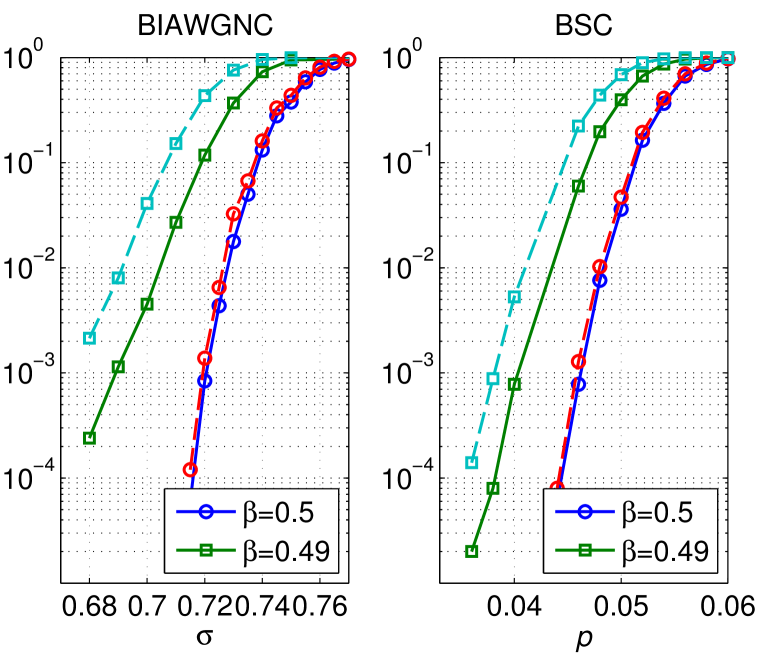
Figure 1: The WER (solid lines) of the WMS algorithm for $(3,6)$-regular LDPC code and the probability of converging to inconsistent messages (dashed lines).

To get the lower bound of the LP decoding threshold, a DE-type analysis is employed in [16] and [17]. The lower bound provided by the DE-type analysis depends on $\beta$ though and is plotted in Figure 2. It is worth noting that according to our simulation result, the best lower bounds, in all cases, are obtained when $\beta=\frac{1}{d_{v}-1}$, and that there is no threshold effect when $\beta<\frac{1}{d_{v}-1}$. The threshold effect does not occur because the density of the correlation between the best skinny trees and the channel output in [16, 17] converges to a fixed point instead of diverging to $\pm\infty.$

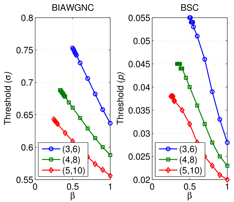
Figure 2: The lower bound of the LP decoding threshold for $(3,6)$, $(4,8)$ and $(5,10)$-regular LDPC codes over BIAWGNC and BSC.

The comparisons of the WER performance between the WMS algorithm and the TRMP algorithm are shown in Figure 3. For any strictly positive pairwise Markov random field (MRF) with binary variables, it has been shown that the fixed point of the TRMP algorithm always specifies an optimal dual solution [10, 20]. The TRMP message update rules in logarithm domain is

$$\nu_{i\rightarrow j}^{(\ell+1)} =\gamma_{i}+\rho\sum_{k\in N\left(i\right)\setminus j}\nu_{i\leftarrow k}^{(\ell)}-\left(1-\rho\right)\nu_{i\leftarrow j}^{(\ell)},$$

$$\nu_{i\leftarrow j}^{(\ell+1)} =\rho\left(\prod_{m\in N(j)\setminus i}\operatorname*{sgn}\left(\nu_{m\rightarrow j}^{(\ell)}\right)\right)\min_{m^{\prime}\in N(j)\setminus i}\left|\nu_{m^{\prime}\rightarrow j}^{(\ell)}\right|-\left(1-\rho\right)\nu_{i\rightarrow j}^{(\ell)},$$

where $\rho\leq 1$ is the edge appearance probability. An uniform edge appearance probability $\rho=\frac{n(1+d_{c}/d_{v})-1}{|\mathcal{E}|}$ is employed in our simulation. One can notice that these update rules are similar to the WMS algorithms. Although, the factor graph for LDPC code is not strictly positive, the optimality of the TRMP hard decisions is observed in a numerical simulation of a $(3,4)$-regular LDPC code with $n=12$. Thus, we take the TRMP algorithm into consideration, and compare its WER performance with the WER performance of the WMS algorithms.

In this comparison, a $(3,6)$-regular LDPC codes over BSC is considered, and the codeword length for both algorithms is $n=10^{4}.$ Three weight factors for the WMS algorithm are tested: $\beta=0.5$, which is discussed in this paper; $\beta=0.8$, which has been shown to have best performance by DE analysis [18]; and $\beta=1$, which is equivalent to the conventional min-sum algorithm for LDPC codes. All WMS algorithms perform $100$ iterations in decoding a codeword. In TRMP algorithm, two simulations with $100$ iterations and $1000$ iterations, respectively, for decoding a codeword are conducted. As shown in Figure 3, the WER performance of the TRMP algorithm with $1000$ iterations is close to the WMS algorithm with $\beta=1$. However, if the TRMP algorithm only performs $100$ iterations in decoding each codeword, it becomes close to the WMS algorithm with $\beta=0.5$. The performance loss of the TRMP algorithm with $100$ iterations is caused by the insufficient number of iterations. Since the TRMP algorithm is not close enough to the converged point, the corresponding hard decision bits are not reliable. Although TRMP algorithm over binary alphabet has been shown LP optimal when the algorithm converges, finding the noise threshold of the TRMP algorithm is still an open problem.

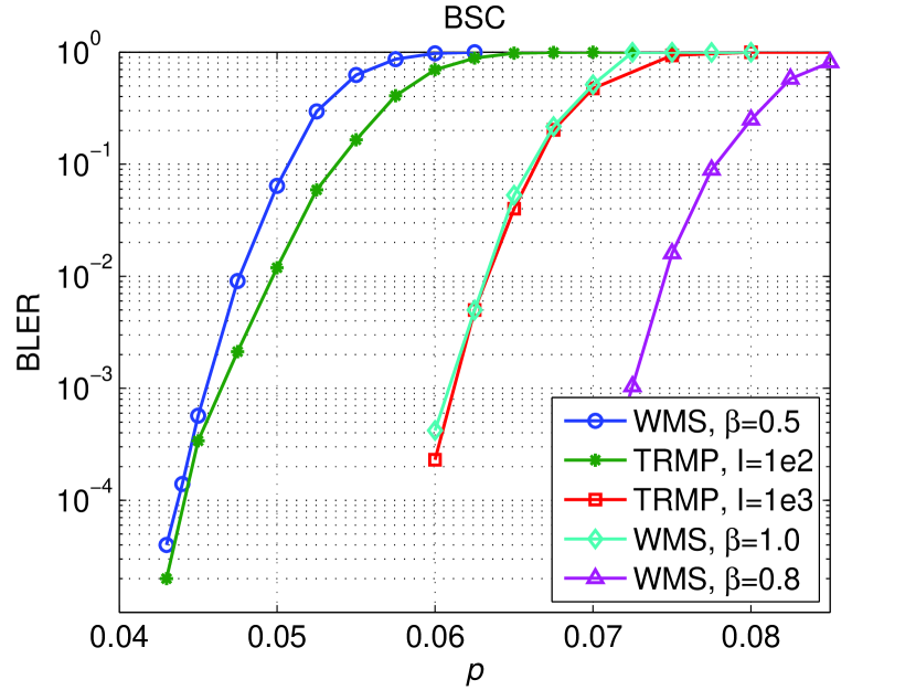
Figure 3: WER performance comparisons for a $(3,6)$-regular LDPC code over the BSC.

VI Conclusions and Future Work

For $(d_{v},d_{c})$-regular LDPC codes, both the attenuated max-product (AMP) algorithm and the weighted min-sum (WMS) algorithm are studied. By slightly modifying the objective function of the original AMP problem in (3) to an equivalent problem in (8), we show that the AMP messages will converge to a fixed point when $\beta<\frac{1}{(d_{v}-1)(d_{c}-1)}$. Further, a set of sufficient conditions (AMP-consistency) for testing the optimality of the AMP solutions is proposed. With the modified AMP problem in (8), we show the LP and ML optimality of the AMP solution by a simple proof if $\beta<\frac{1}{(d_{v}-1)(d_{c}-1)}$ and the fixed point is AMP-consistent

Similarly, when the weight factor $\beta<\frac{1}{d_{v}-1},$ we show that the WMS algorithm converges to a unique fixed point. We also introduce the sufficient conditions (WMS-consistency) for the hard decisions of the WMS algorithm to be a valid codeword. By employing the construction of a dual feasible point of the LP decoding (Problem-P) in [15], we show that if $\beta<\frac{1}{d_{v}-1}$ and the WMS algorithm converges to a consistent codeword, we can simplify the construction by using the converged messages. Also, we show that the dual feasible point obtained by the converged messages is an optimal dual feasible point, and the corresponding hard decisions are the LP optimum as well as the ML solution. Based on the analysis of the WMS algorithm with $\beta<\frac{1}{d_{v}-1}$, the optimality of the WMS algorithm with $\beta=\frac{1}{d_{v}-1}$ is also discussed. When the WMS messages with $\beta=\frac{1}{d_{v}-1}$ satisfy the consistency conditions and diverge to $\pm\infty$, we show that the hard decisions is ML optimum as well. This result can be seen as the natural completion of the work initiated by Koetter and Frey in [7]. Also, our results have interesting connections with the results of [16] because their best LP thresholds also occur when $\beta=\frac{1}{d_{v}-1}$ according to DE analysis. For weight factors $\beta>\frac{1}{d_{v}-1},$ we provide a counterexample which shows that it is not always possible to provide ML certificates for WMS decoding.

In regards to future work, the most interesting open question is whether connections between LP decoding and WMS decoding can be extended beyond $\beta=\frac{1}{d_{v}-1}$. In [18], Chen et al. studied the optimal attenuation factor for the WMS algorithm. For example, the best $\beta$ for the $(3,6)$-regular LDPC code on the BSC is $\beta=0.8,$ and the corresponding threshold is $p=0.083$. DE also shows that any extension beyond $\beta=\frac{1}{d_{v}-1}$ will provide an improved lower bound on the LP threshold. Moreover, the construction of an optimal dual-feasible point for the LP decoding on an irregular LDPC code using WMS messages is still unclear to us. Let $d_{v,i}$ be the degree of the $i$th bit. With the construction proposed in this paper, we need $\beta_{i}=\beta<\min_{i^{\prime}\in\mathcal{V}_{L}}\{\frac{1}{d_{v,i^{\prime}}-1}\}$ for all $i\in\mathcal{V}_{L}$ to ensure the convergence of WMS messages and the optimality of the corresponding dual-feasible point. However, there exists no threshold for the WMS algorithm with this choice of $\beta_{i}$. Therefore, a general weighting strategy and the corresponding construction of the optimal dual-feasible point for irregular LDPC codes is still an open problem. Since the irregular LDPC code has been proved to be capacity-approaching in [4], we expect that the irregular LDPC code with general weighting scheme can improve current estimate of the noise threshold for the LP decoding over a rate-$\frac{1}{2}$ LDPC code.

Appendix A Proof of Lemma 3

Proof:

Let $\ell,\,m\leq n$ be the integers such that $f_{\ell}=\max_{i}f_{i}$ and $g_{m}=\max_{i}g_{i}$. If $f_{\ell}\geq g_{m}$, it can be shown that $f_{\ell}-g_{i}\geq 0$ for all $i=1,2,\dots,n$. Thus, it follows that

$$\max_{i}\left|f_{i}-g_{i}\right| \geq\left|f_{\ell}-g_{\ell}\right|=f_{\ell}-g_{\ell}\geq f_{\ell}-g_{m}=\left|f_{\ell}-g_{m}\right|.$$

On the other hand, if $f_{\ell}\leq g_{m}$, we still can have the same inequality by

$$\max_{i}\left|f_{i}-g_{i}\right| \geq\left|f_{m}-g_{m}\right|=g_{m}-f_{m}\geq g_{m}-f_{\ell}=\left|f_{\ell}-g_{m}\right|.$$

Therefore, we obtain (16). ∎

Appendix B Proof of Lemma 7

Proof:

By the definition of the DP value function in (9), we have

$$\sum_{(i,j)\in\mathcal{E}}\mu_{i\rightarrow j}^{*}\left(x_{i,j}\right) =\sum_{(i,j)\in\mathcal{E}}\left(1-x_{i,j}\right)\gamma_{i}+\beta\sum_{\begin{subarray}{c}(i,j)\in\mathcal{E}\\ k\in N(i)\backslash j\end{subarray}}\max_{\boldsymbol{w}\in\mathcal{S}_{k,i}(x_{i,j})}\sum_{m\in N(k)\backslash i}\mu_{m\rightarrow k}^{*}\left(w_{m}\right),$$ (34)

where $\mathcal{S}_{k,i}(x_{i,j})$ is defined in (6). Since $x_{i,j}^{*}$ maximizes $\mu_{i\rightarrow j}^{*}(x)$, the inequality can be obtained by simply replacing $w_{m}$ in (34) with $x_{m,k}^{*}$. Thus, we have

$$\sum_{(i,j)\in\mathcal{E}}\mu_{i\rightarrow j}^{*}(x_{i,j}) \leq\sum_{(i,j)\in\mathcal{E}}(1-x_{i,j})\gamma_{i}+\beta\sum_{\begin{subarray}{c}(i,j)\in\mathcal{E},\,k\in N(i)\backslash j,\\ m\in N(k)\backslash i\end{subarray}}\mu_{m\rightarrow k}^{*}\left(x_{m,k}^{*}\right)$$

$$=\sum_{(i,j)\in\mathcal{E}}\left(1-x_{i,j}\right)\gamma_{i}+\beta\left(d_{v}-1\right)\left(d_{c}-1\right)\sum_{(i,j)\in\mathcal{E}}\mu_{i\rightarrow j}^{*}\left(x_{i,j}^{*}\right).$$

To show the equality, by substituting $x_{i,j}^{*}$ into (34), we have

$$\sum_{(i,j)\in\mathcal{E}}\mu_{i\rightarrow j}^{*}\left(x_{i,j}^{*}\right) =\sum_{(i,j)\in\mathcal{E}}\left(1-x_{i,j}^{*}\right)\gamma_{i}+\beta\sum_{\begin{subarray}{c}(i,j)\in\mathcal{E}\\ k\in N(i)\backslash j\end{subarray}}\max_{\boldsymbol{w}\in\mathcal{S}_{k,i}(x_{i,j}^{*})}\sum_{m\in N(k)\backslash i}\mu_{m\rightarrow k}^{*}\left(w_{m}\right).$$ (35)

Since $\{x_{i,j}^{*}\}$ is AMP-consistent, there exists a vector $\boldsymbol{x}^{*}\in\mathcal{C}$ such that $x_{i}^{*}=x_{i,j}^{*}$ for all $i\in\mathcal{V}_{L}$ and $j\in N(i)$. By the fact that $\boldsymbol{x}^{*}\in\mathcal{S}_{k,i}(x_{i,j}^{*})$, the last term in equation (35) is equal to

$$\beta\sum_{\begin{subarray}{c}(i,j)\in\mathcal{E},\,k\in N(i)\backslash j,\\ m\in N(k)\backslash i\end{subarray}}\mu_{m\rightarrow k}^{*}\left(x_{m,k}^{*}\right).$$

Therefore, we obtain the equality. ∎

Appendix C Proof of Lemma 12

Proof:

Since $\prod_{m\in N(k)\setminus i}\operatorname*{sgn}(\mu_{m\rightarrow k})\operatorname*{sgn}(\nu_{m\rightarrow k})$ can be $\pm 1$, we must show that

$$\max_{m\in N(k)\backslash i}\left|\mu_{m\rightarrow k}-\nu_{m\rightarrow k}\right| \geq\left|\min_{m\in N(k)\backslash i}\left|\mu_{m\rightarrow k}\right|-\min_{m\in N(k)\backslash i}\left|\nu_{m\rightarrow k}\right|\right|,$$ (36)

when all $\mu_{m\rightarrow k},\nu_{m\rightarrow k}$ signs match on $m\in N(k)\setminus i,$ and

$$\max_{m\in N(k)\backslash i}\left|\mu_{m\rightarrow k}-\nu_{m\rightarrow k}\right| \geq\left|\min_{m\in N(k)\backslash i}\left|\mu_{m\rightarrow k}\right|+\min_{m\in N(k)\backslash i}\left|\nu_{m\rightarrow k}\right|\right|,$$ (37)

when some signs differ.

To show (36), define the following indices

$$m_{1} \triangleq\operatorname*{arg\,min}_{m\in N(k)\setminus i}\left|\mu_{m\rightarrow k}\right|,$$

$$m_{2} \triangleq\operatorname*{arg\,min}_{m\in N(k)\setminus i}\left|\nu_{m\rightarrow k}\right|,$$

and

$$m^{\star}\triangleq\operatorname*{arg\,max}_{m\in N(k)\backslash i}\left|\mu_{m\rightarrow k}-\nu_{m\rightarrow k}\right|.$$

Notice that

$$\left|\mu_{m^{\star}\rightarrow k}-\nu_{m^{\star}\rightarrow k}\right| \geq\max_{m\in N(k)\setminus i}\left||\mu_{m\rightarrow k}|-|\nu_{m\rightarrow k}|\right|$$

$$=\max_{m\in N(k)\setminus i}\left||\nu_{m\rightarrow k}|-|\mu_{m\rightarrow k}|\right|.$$

Consider the case when $|\mu_{m_{1}\rightarrow k}|\geq|\nu_{m_{2}\rightarrow k}|$. Since $|\mu_{m_{2}\rightarrow k}|\geq|\mu_{m_{1}\rightarrow k}|\geq|\nu_{m_{2}\rightarrow k}|$, it follows that

$$\left|\mu_{m^{\star}\rightarrow k}-\nu_{m^{\star}\rightarrow k}\right| \geq\max_{m\in N(k)\setminus i}\left||\mu_{m\rightarrow k}|-|\nu_{m\rightarrow k}|\right|$$

$$\geq\left||\mu_{m_{2}\rightarrow k}|-|\nu_{m_{2}\rightarrow k}|\right|$$

$$\geq\left||\mu_{m_{1}\rightarrow k}|-|\nu_{m_{2}\rightarrow k}|\right|.$$ (38)

When $|\mu_{m_{1}\rightarrow k}|\leq|\nu_{m_{2}\rightarrow k}|$, we know $|\mu_{m_{1}\rightarrow k}|\leq|\nu_{m_{2}\rightarrow k}|\leq|\nu_{m_{1}\rightarrow k}|$. It can be shown that

$$\max_{m\in N(k)\setminus i}\left||\mu_{m\rightarrow k}|-|\nu_{m\rightarrow k}|\right| \geq\left||\nu_{m_{1}\rightarrow k}|-|\mu_{m_{1}\rightarrow k}|\right|$$

$$\geq\left||\nu_{m_{2}\rightarrow k}|-|\mu_{m_{1}\rightarrow k}|\right|$$

$$\geq\left||\mu_{m_{1}\rightarrow k}|-|\nu_{m_{2}\rightarrow k}|\right|,$$ (39)

and combining the results in (38) and (39) implies (36).

To show (37), let $\mathcal{M}=\{m\in N(k)\setminus i:\,\mu_{m\rightarrow k}\nu_{m\rightarrow k}<0\}$ be the set of indices such that $\mu_{m\rightarrow k}$ and $\nu_{m\rightarrow k}$ have different signs. Notice that

$$\max_{m\in N(k)\setminus i}\left|\mu_{m\rightarrow k}-\nu_{m\rightarrow k}\right| \geq\max_{m\in\mathcal{M}}\left|\mu_{m\rightarrow k}-\nu_{m\rightarrow k}\right|$$

$$\geq\max_{m\in\mathcal{M}}\left||\mu_{m\rightarrow k}|+|\nu_{m\rightarrow k}|\right|$$

$$\geq\left|\min_{m\in\mathcal{M}}|\mu_{m\rightarrow k}|+\min_{m\in\mathcal{M}}|\nu_{m\rightarrow k}|\right|$$

$$\geq\left|\min_{m\in N(k)\setminus i}|\mu_{m\rightarrow k}|+\min_{m\in N(k)\setminus i}|\nu_{m\rightarrow k}|\right|.$$

This completes the proof. ∎

Appendix D Proof of Lemma 21

Proof:

Let $\boldsymbol{\mu}^{\prime}\triangleq\mathsf{W}_{\delta}[\boldsymbol{\mu}]$ and $\boldsymbol{\nu}^{\prime}\triangleq\mathsf{W}_{\delta}[\boldsymbol{\nu}]$. One can compute the sign of the check-to-bit messages for each edge $(i,j)\in\mathcal{E}$ with $\operatorname*{sgn}(\mu_{i\leftarrow j})=\prod_{m\in N(j)\setminus i}\operatorname*{sgn}(\mu_{m\rightarrow j}$) and $\operatorname*{sgn}(\nu_{i\leftarrow j})=\prod_{m\in N(j)\setminus i}\operatorname*{sgn}(\nu_{m\rightarrow j}$). Using this and $\boldsymbol{\mu}\overset{s}{=}\boldsymbol{\nu}$, it follows that

$$\operatorname*{sgn}(\mu_{i\leftarrow j})=\operatorname*{sgn}(\nu_{i\leftarrow j})$$ (40)

for all $(i,j)\in\mathcal{E}$.

Since $\boldsymbol{\mu},\,\boldsymbol{\nu}$ both satisfy the consistency conditions, we know that $\operatorname*{sgn}(\mu_{i\leftarrow j})=\operatorname*{sgn}(\mu_{i\leftarrow j^{\prime}})$ and $\operatorname*{sgn}(\nu_{i\leftarrow j})=\operatorname*{sgn}(\nu_{i\leftarrow j^{\prime}})$ for all $j,\,j^{\prime}\in N(i)$. Thus, for each $(i,\,j)\in\mathcal{E}$, $\mu_{i\rightarrow j}^{\prime}$ and $\nu^{\prime}_{i\rightarrow j}$ can be expressed as

$$\mu_{i\rightarrow j}^{\prime} =\operatorname*{sgn}\left(\mu_{i\leftarrow j}\right)\left(\operatorname*{sgn}\left(\mu_{i\leftarrow j}\right)\gamma_{i}+\frac{\delta}{d_{v}-1}\sum_{k\in N(i)\setminus j}\min_{m^{\prime}\in N(k)\setminus i}\left|\mu_{m^{\prime}\rightarrow k}\right|\right)$$ (41)

and

$$\nu_{i\rightarrow j}^{\prime} =\operatorname*{sgn}\left(\nu_{i\leftarrow j}\right)\left(\operatorname*{sgn}\left(\nu_{i\leftarrow j}\right)\gamma_{i}+\frac{\delta}{d_{v}-1}\sum_{k\in N(i)\setminus j}\min_{m^{\prime}\in N(k)\setminus i}\left|\nu_{m^{\prime}\rightarrow k}\right|\right).$$ (42)

Since $|\boldsymbol{\nu}|\succeq\frac{\|\boldsymbol{\gamma}\|_{\infty}}{\delta}\boldsymbol{1}$, we have

$$\operatorname*{sgn}\left(\nu_{i\leftarrow j}\right)\gamma_{i}+\frac{\delta}{d_{v}-1}\sum_{k\in N(i)\setminus j}\min_{m^{\prime}\in N(k)\setminus i}\left|\nu_{m^{\prime}\rightarrow k}\right|$$

$$\phantom{\operatorname*{sgn}\left(\nu_{i\leftarrow j}\right)\gamma_{i}+\frac{\delta}{d_{v}-1}}\geq\operatorname*{sgn}\left(\nu_{i\leftarrow j}\right)\gamma_{i}+\|\boldsymbol{\gamma}\|_{\infty}\geq 0.$$ (43)

Hence,

$$\left|\nu^{\prime}_{i\rightarrow j}\right| =\operatorname*{sgn}\left(\nu_{i\leftarrow j}\right)\gamma_{i}+\frac{\delta}{d_{v}-1}\sum_{k\in N(i)\setminus j}\min_{m^{\prime}\in N(k)\setminus i}\left|\nu_{m^{\prime}\rightarrow k}\right|$$

and similarly,

$$\left|\mu^{\prime}_{i\rightarrow j}\right| =\operatorname*{sgn}\left(\mu_{i\leftarrow j}\right)\gamma_{i}+\frac{\delta}{d_{v}-1}\sum_{k\in N(i)\setminus j}\min_{m^{\prime}\in N(k)\setminus i}\left|\mu_{m^{\prime}\rightarrow k}\right|.$$

By $|\boldsymbol{\mu}|\succeq|\boldsymbol{\nu}|$ and (40), we have $|\boldsymbol{\mu}^{\prime}|\succeq|\boldsymbol{\nu}^{\prime}|$.

Moreover, from (41), (42) and (43), the signs of $\mu^{\prime}_{i\rightarrow j}$ and $\nu^{\prime}_{i\rightarrow j}$ satisfy $\operatorname*{sgn}(\nu^{\prime}_{i\rightarrow j})=\operatorname*{sgn}(\nu_{i\leftarrow j})$ and $\operatorname*{sgn}(\mu^{\prime}_{i\rightarrow j})=\operatorname*{sgn}(\mu_{i\leftarrow j})$. By the consistency property of $\boldsymbol{\mu}$ and $\boldsymbol{\nu}$, we know $\operatorname*{sgn}(\nu^{\prime}_{i\rightarrow j})=\operatorname*{sgn}(\nu_{i\leftarrow j})=\operatorname*{sgn}(\nu_{i\rightarrow j})$ and $\operatorname*{sgn}(\mu^{\prime}_{i\rightarrow j})=\operatorname*{sgn}(\mu_{i\leftarrow j})=\operatorname*{sgn}(\mu_{i\rightarrow j})$ for all $(i,j)\in\mathcal{E}$. This concludes the proof. ∎

Appendix E Proof of Lemma 27

Proof:

From (11), the absolute value of the difference $\mu_{i\rightarrow j}^{(\ell)}-\mu_{\delta,i\rightarrow j}^{(\ell)}$ in the $\ell$th iteration can be written as

$$\left|\mu_{i\rightarrow j}^{(\ell)}-\mu_{\delta,i\rightarrow j}^{(\ell)}\right| =\left|\frac{1}{d_{v}-1}\sum_{k\in N(i)\setminus j}\mu_{i\leftarrow k}^{(\ell-1)}-\frac{\delta}{d_{v}-1}\sum_{k^{\prime}\in N(i)\setminus j}\mu_{\delta,i\leftarrow k^{\prime}}^{(\ell-1)}\right|.$$ (44)

By triangle inequality, (44) is upper bounded by

$$\frac{\delta}{d_{v}-1}\sum_{k\in N(i)\setminus j}\left|\mu_{i\leftarrow k}^{(\ell-1)}-\mu_{\delta,i\leftarrow k}^{(\ell-1)}\right|+\frac{1-\delta}{d_{v}-1}\sum_{k^{\prime}\in N(i)\setminus j}\left|\mu_{i\leftarrow k^{\prime}}^{(\ell-1)}\right|.$$

From Lemma 12 and (12), we know $|\mu_{i\leftarrow k}^{(\ell-1)}-\mu_{\delta,i\leftarrow k}^{(\ell-1)}|\leq\max_{m\in N(k)\setminus i}|\mu_{m\rightarrow k}^{(\ell-1)}-\mu_{\delta,m\rightarrow k}^{(\ell-1)}|$. Also, by the fact that $|\mu_{i\leftarrow k^{\prime}}^{(\ell-1)}|=\min_{m\in N(k^{\prime})\setminus i}|\mu_{m\rightarrow k^{\prime}}^{(\ell-1)}|$, we can further upper bound (44) by

$$\frac{\delta}{d_{v}-1}\sum_{k\in N(i)\setminus j}\max_{m\in N(k)\setminus i}\left|\mu_{m\rightarrow k}^{(\ell-1)}-\mu_{\delta,m\rightarrow k}^{(\ell-1)}\right|$$

$$\phantom{\frac{\delta}{d_{v}-1}\sum_{k\in N(i)\setminus j}}+\frac{1-\delta}{d_{v}-1}\sum_{k^{\prime}\in N(i)\setminus j}\min_{m\in N(k^{\prime})\setminus i}\left|\mu_{m\rightarrow k^{\prime}}^{(\ell-1)}\right|.$$

Since $|\mu_{i\rightarrow j}^{(\ell-1)}-\mu_{\delta,i\rightarrow j}^{(\ell-1)}|\leq\|\boldsymbol{\mu}^{(\ell-1)}-\boldsymbol{\mu}_{\delta}^{(\ell-1)}\|_{\infty}$ and $|\mu_{i\rightarrow j}^{(\ell-1)}|\leq\ell\|\boldsymbol{\gamma}\|_{\infty}$ for all $(i,j)\in\mathcal{E}$, we have

$$\left|\mu_{i\rightarrow j}^{(\ell)}-\mu_{\delta,i\rightarrow j}^{(\ell)}\right| \leq\frac{\delta}{d_{v}-1}\sum_{k\in N(i)\setminus j}\left\|\boldsymbol{\mu}^{(\ell-1)}-\boldsymbol{\mu}_{\delta}^{(\ell-1)}\right\|_{\infty}+\frac{1-\delta}{d_{v}-1}\sum_{k^{\prime}\in N(i)\setminus j}\ell\|\boldsymbol{\gamma}\|_{\infty}$$

$$\leq\left\|\boldsymbol{\mu}^{(\ell-1)}-\boldsymbol{\mu}_{\delta}^{(\ell-1)}\right\|_{\infty}+(1-\delta)\ell\|\boldsymbol{\gamma}\|_{\infty}.$$ (45)

Since the RHS of (45) is a constant with respect to $(i,j)\in\mathcal{E}$, one gets the recursive upper bound

$$\left\|\boldsymbol{\mu}^{(\ell)}-\boldsymbol{\mu}_{\delta}^{(\ell)}\right\|_{\infty} \leq\left\|\boldsymbol{\mu}^{(\ell-1)}-\boldsymbol{\mu}_{\delta}^{(\ell-1)}\right\|_{\infty}+(1-\delta)\ell\|\boldsymbol{\gamma}\|_{\infty}.$$ (46)

Note that $|\mu_{i\rightarrow j}^{(0)}-\mu_{\delta,i\rightarrow j}^{(0)}|=0$. For a given $\ell\leq L$, we can apply (46) recursively, and have

$$\left\|\boldsymbol{\mu}^{(\ell)}-\boldsymbol{\mu}_{\delta}^{(\ell)}\right\|_{\infty} <(1-\delta)\frac{\ell\left(\ell+1\right)}{2}\|\boldsymbol{\gamma}\|_{\infty}$$

$$\leq(1-\delta)\frac{L\left(L+1\right)}{2}\|\boldsymbol{\gamma}\|_{\infty},$$

for all $\ell\leq L$. Therefore, for any fixed $\epsilon>0$, if we choose

$$\delta \geq 1-\frac{2\epsilon}{L\left(L+1\right)\|\boldsymbol{\gamma}\|_{\infty}},$$ (47)

then $|\mu_{i\rightarrow j}^{(\ell)}-\mu_{\delta,i\rightarrow j}^{(\ell)}|\leq\|\boldsymbol{\mu}^{(\ell)}-\boldsymbol{\mu}_{\delta}^{(\ell)}\|_{\infty}<\epsilon$ for all $\ell\leq L$. ∎

Appendix F Extensions of the Work in [16]

In this appendix, we briefly recall the main idea and statement in our earlier work in [19], and provide detail proves of lemmas, which were omitted in [19]. We extend the lemmas and theorems in [16] to the case when the depth of the computation tree exceeds $\frac{1}{2}\mbox{girth}(\mathcal{G})$. With these extended results, another proof of the conclusion drawn in Section III-B is obtained.

Since a computation tree with depth greater than $\frac{1}{2}\mbox{girth}(\mathcal{G})$ is considered in this section, we generalize the definition in Section II-B as follows. Let $\mathcal{T}_{i_{0}}^{2T}=(\mathcal{I}\cup\mathcal{J},\mathcal{E}^{\prime})$ be a depth-$2T$ computation tree and rooted at $i_{0}\in\mathcal{V}_{L}$, where $\mathcal{I}$ and $\mathcal{J}$ are the set of variable nodes and the set of check nodes in $\mathcal{T}_{i_{0}}^{2L}$, respectively, and $T\geq\frac{1}{4}\mbox{girth}(\mathcal{G})$. Let $i^{{}^{\prime}}$ and $j^{{}^{\prime}}$ denote a variable node and a check node in $\mathcal{T}_{i_{0}}^{2T}$, respectively. We say that $i^{\prime}$ is associated with the bit $i\in\mathcal{V}_{L}$ in $\mathcal{G}$ (denoted $i^{\prime}\sim i$) if $i^{\prime}$ is a copy of $i$. Similarly, $j^{\prime}\sim j$ denotes that $j^{\prime}\in\mathcal{J}$ is a copy of $j\in\mathcal{V}_{R}$. Moreover, we define two projections $\eta:\mathcal{I}\rightarrow\mathcal{V}_{L}$ and $\theta:\mathcal{J}\rightarrow\mathcal{V}_{R}$ by $\eta(i^{{}^{\prime}})=\{i\in\mathcal{V}_{L}:i^{{}^{\prime}}\sim i\}$ and $\theta(j^{{}^{\prime}})=\{j\in\mathcal{V}_{R}:j^{{}^{\prime}}\sim j\}$.

At first, we generalize the definitions from [5] and [16, Definition 1] as follows.

Definition 35.

Consider a computation tree $\mathcal{T}_{i_{0}}^{2T}=(\mathcal{I}\cup\mathcal{J},\mathcal{E^{\prime}})$ of depth $2T\geq\frac{1}{2}\mbox{girth}(\mathcal{G})$ and rooted at $i_{0}$. A bit assignment $\boldsymbol{u}\in\{0,1\}^{|\mathcal{I}|}$ on $\mathcal{T}_{i_{0}}^{2T}$ is a generalized valid deviation of depth $T$ at $i_{0}\in\mathcal{V}_{L}$ or, in short, a generalized $T$-local deviation at $i_{0}$, if $u_{i_{0}}=1$ and $\boldsymbol{u}$ satisfies all parity checks in $\mathcal{T}_{i_{0}}^{2T}$. Moreover, $\boldsymbol{u}$ is a generalized minimal $T$-local deviation if, for every check node $j\in\mathcal{T}_{i_{0}}^{2T}$, at most two neighbor bits are assigned the value $1$. Note that a generalized minimal $T$-local deviation at $i_{0}$ can be seen as a subtree of $\mathcal{T}_{i_{0}}^{2T}$ of depth $2T$ rooted at $i_{0},$ where every variable node has full degree and every check node has degree $2$. Such a tree is referred as a skinny tree. If $\boldsymbol{\varpi}=(\varpi_{0},\dots,\varpi_{T})\in[0,1]^{T}$ is a weight vector and $\boldsymbol{u}$ is a generalized minimal $T$-local deviation at $i_{0}$, then $\boldsymbol{u}^{(\varpi)}$ denotes the $\varpi$-weighted deviation

$$u_{i}^{(\varpi)}=\begin{cases}\varpi_{t}u_{i}&\mbox{ if }i\in N\left(i_{0},2t\right)\mbox{ and }0\leq t\leq T,\\ 0&\mbox{ otherwise.}\end{cases}$$

For any $\varpi$-weighted deviation $\boldsymbol{u}^{(\varpi)}$ on $\mathcal{T}_{i_{0}}^{2T}$, let the projection of $\boldsymbol{u}^{(\varpi)}$ onto the code bit $i\in\mathcal{V}_{L}$ be

$$\pi_{i}\left(\boldsymbol{u}^{(\varpi)}\right)=\sum_{t=0}^{T}\varpi_{t}\sum_{m\in N(i_{0},2t):\,m\sim i}u_{m}.$$

Likewise, we let $\pi\left(\boldsymbol{u}^{(\varpi)}\right)$ represent the vector whose elements are $\pi_{i}\left(\boldsymbol{u}^{(\varpi)}\right)$ for $i\in\mathcal{V}_{L}$. The weights are chosen to be $\varpi_{t}=\beta^{t}$ for some $\beta\in[0,1].$

To extend the results of [16] to the computation trees of depth $I\rightarrow\infty$, we utilize the following fact that, for each $i_{0}\in\mathcal{V}_{L}$, the WMS algorithm computes the best assignment, $\tilde{x}_{i_{0}}$, for the root of $\mathcal{T}_{i_{0}}^{2I}$, and there is a corresponding best assignment $\tilde{\boldsymbol{x}}$ for the tree $\mathcal{T}_{i_{0}}^{2I}$. In the following lemma, a weighted correlation between $\tilde{\boldsymbol{x}}$ and a generalized minimal $I$-local deviation is introduced. Since $\tilde{\boldsymbol{x}}$ is the best assignment, it can be shown that the weighted correlation is positive when the number of iterations is large enough.

Lemma 36.

Given the LLR vector $\boldsymbol{\gamma}\in\mathbb{R}^{n},$ let the assignment $\tilde{\boldsymbol{x}}$ for the computation tree $\mathcal{T}_{i_{0}}^{2I}$, computed by the WMS decoding with $\beta<\frac{1}{d_{v}-1}$, be unique (i.e., there are no ties) after $I\rightarrow\infty$ iterations. Let $\tilde{\boldsymbol{x}}$ be the corresponding assignment for $\mathcal{T}_{i_{0}}^{2I}$. For any generalized minimal $I$-local deviation, $\tilde{\boldsymbol{u}}$, rooted at $i_{0}$ and any $T\ll I$, let the $T$-level weighted correlation be

$$U_{i_{0}}^{T}(\tilde{\boldsymbol{x}},\tilde{\boldsymbol{u}})\triangleq\sum_{i=1}^{n}\sum_{t=0}^{T}\beta^{t}\sum_{m\in N(i_{0},2t):\,m\sim i}(-1)^{\tilde{x}_{m}}\tilde{u}_{m}\gamma_{i},$$ (48)

where $N(i_{0},\ell)$ is the set of vertices in the $\ell$th level of $\mathcal{T}_{i_{0}}^{2I}.$ Then, there exists a $T_{0}<\infty$ such that $U_{i_{0}}^{T}(\tilde{\boldsymbol{x}},\tilde{\boldsymbol{u}})>0$ for all $T\geq T_{0}$ and for all $\tilde{\boldsymbol{u}}$.

Proof:

Since $\tilde{\boldsymbol{x}}$ is the optimal WMS assignment for the computation tree $\mathcal{T}_{i_{0}}^{2I}$ after $I$ iterations, there exists an $\epsilon>0$ such that, for all generalized minimal $I$-local deviations $\tilde{\boldsymbol{u}}$, we have

$$V_{i_{0}}^{I}(\tilde{\boldsymbol{x}}) =\sum_{i=1}^{n}\left(\sum_{t=0}^{I}\beta^{t}\sum_{m\in N(i_{0},2t):m\sim i}\tilde{x}_{m}\right)\gamma_{i}$$

$$<-\epsilon+\sum_{i=1}^{n}\left(\sum_{t=0}^{I}\beta^{t}\sum_{m\in N(i_{0},2t):m\sim i}(\tilde{x}_{m}\oplus\tilde{u}_{m})\right)\gamma_{i}$$

$$=-\epsilon+\sum_{i=1}^{n}\left(\sum_{t=0}^{I}\beta^{t}\left(\sum_{m\in N(i_{0},2t):m\sim i}\tilde{x}_{m}+\sum_{m\in N(i_{0},2t):m\sim i}(-1)^{\tilde{x}_{m}}\tilde{u}_{m}\right)\right)\gamma_{i}$$

$$=-\epsilon+V_{i_{0}}^{I}(\tilde{\boldsymbol{x}})+\sum_{i=1}^{n}\left(\sum_{t=0}^{I}\beta^{t}\sum_{m\in N(i_{0},2t):m\sim i}(-1)^{\tilde{x}_{m}}\tilde{u}_{m}\right)\gamma_{i}$$

$$=-\epsilon+V_{i_{0}}^{I}(\tilde{\boldsymbol{x}})+U_{i_{0}}^{T}(\tilde{\boldsymbol{x}},\tilde{\boldsymbol{u}})+R(\tilde{\boldsymbol{x}},\tilde{\boldsymbol{u}}),$$

where

$$R(\tilde{\boldsymbol{x}},\tilde{\boldsymbol{u}})=\sum_{i=1}^{n}\left(\sum_{t=T+1}^{I}\beta^{t}\sum_{m\in N(i_{0},2t):m\sim i}(-1)^{\tilde{x}_{m}}\tilde{u}_{m}\right)\gamma_{i},$$

and $\tilde{x}_{m}\oplus\tilde{u}_{m}$ is the sum of $\tilde{x}_{m}$ and $\tilde{u}_{m}$ modulo $2$. The $|R(\tilde{\boldsymbol{x}},\tilde{\boldsymbol{u}})|$ can be upper bounded by

$$|R(\tilde{\boldsymbol{x}},\tilde{\boldsymbol{u}})| \leq\sum_{i=1}^{n}\sum_{t=T+1}^{I}\beta^{t}\sum_{m\in N(i_{0},2t):m\sim i}\tilde{u}_{m}|\gamma_{i}|$$

$$\leq\|\boldsymbol{\gamma}\|_{\infty}\left(\sum_{i=1}^{n}\sum_{t=T+1}^{I}\beta^{t}\sum_{m\in N(i_{0},2t):m\sim i}\tilde{u}_{m}\right)$$

$$=\|\boldsymbol{\gamma}\|_{\infty}\left(\sum_{t=T+1}^{I}\beta^{t}d_{v}\left(d_{v}-1\right)^{t-1}\right)$$

$$\leq\|\boldsymbol{\gamma}\|_{\infty}\beta^{T}d_{v}(d_{v}-1)^{T-1}\left(\sum_{t=1}^{I-T}\beta^{t}(d_{v}-1)^{t}\right).$$

Since $\beta<\frac{1}{d_{v}-1}$, it follows that $R(\tilde{\boldsymbol{x}},\tilde{\boldsymbol{u}})\rightarrow 0$ as $T\rightarrow\infty$. Therefore, we can choose a $T_{0}<\infty$ so that $U_{i_{0}}^{T}(\tilde{\boldsymbol{x}},\tilde{\boldsymbol{u}})>\epsilon-R(\tilde{\boldsymbol{x}},\tilde{\boldsymbol{u}})>0$ for all $T\geq T_{0}$. This completes the proof. ∎

Remark 37.

Let $\tilde{\boldsymbol{x}}$ and $\tilde{\boldsymbol{u}}$ be as defined in Lemma 36, and let $T\geq T_{0}$. Since $U_{i_{0}}^{T}(\tilde{\boldsymbol{x}},\tilde{\boldsymbol{u}})>0$, it follows that $V_{i_{0}}^{T}(\tilde{\boldsymbol{x}}\oplus\tilde{\boldsymbol{u}})=V_{i_{0}}^{T}(\tilde{\boldsymbol{x}})+U_{i_{0}}^{T}(\tilde{\boldsymbol{x}},\tilde{\boldsymbol{u}})>V_{i_{0}}^{T}(\tilde{\boldsymbol{x}})$ for all $\tilde{\boldsymbol{u}}$. This observation implies that, when $\beta<\frac{1}{d_{v}-1}$ and the number of iterations is large, the binary assignments of the leaf nodes are asymptotically irrelevant to the assignment of $\tilde{x}_{i_{0}}$.

The following extends the key result [16, Lemma 4] to our generalized minimal local deviations on the computation tree.

Lemma 38.

Let $\mathcal{P}$ be the fundamental polytope of an LDPC, and $\boldsymbol{z}\in\mathcal{P}$ be a LP solution of a bit-regular code. Consider the set of depth-$I$ computation trees rooted at all non-zero variable nodes. For these trees, there exists a distribution over generalized minimal local deviations such that the expected value, when projected onto the original Tanner graph, is proportional to the LP solution $\boldsymbol{z}$.

Proof:

This fact was first observed in [21, Remark 22]. See Appendix G for a proof based on extending the proof of [16, Lemma 4]. ∎

The following theorem shows that if the WMS messages converge to a WMS-consistent fixed point, then the hard decision bits of the WMS algorithm give a codeword that is both LP optimal and ML.

Theorem 39.

For a given the LLR vector $\boldsymbol{\gamma}\in\mathbb{R}^{n}$ and a weight $0\leq\beta<\frac{1}{d_{v}-1}$, suppose the WMS algorithm converges to a WMS-consistent fixed point. If the hard decision bits $\hat{\boldsymbol{x}}$ are unique (i.e., there are no ties), then they form a $T$-locally optimal codeword for some $T<\infty$. Moreover, $\hat{\boldsymbol{x}}$ is the LP optimal and, hence, ML codeword.

Proof:

From Theorem 11, we know that $\hat{\boldsymbol{x}}$ is a codeword. To prove that $\hat{\boldsymbol{x}}$ is a $T$-locally optimal codeword, we have to show that for the projection $\pi(\boldsymbol{u}^{(\varpi)})$ of any generalized minimal $T$-local deviation $\boldsymbol{u}^{(\varpi)},$ the inequality

$${\textstyle\left\langle\hat{\boldsymbol{x}}\oplus c\pi\left(\boldsymbol{u}^{(\varpi)}\right),\boldsymbol{\gamma}\right\rangle}>\left\langle\hat{\boldsymbol{x}},\boldsymbol{\gamma}\right\rangle$$

holds, where $c>0$ is a scaling factor such that $c\pi_{i}(\boldsymbol{u}^{(\varpi)})\leq 1$ for all $i\in 1,2,\dots,n$, and $(\hat{\boldsymbol{x}}\oplus c\pi(\boldsymbol{u}^{(\varpi)}))_{i}=|\hat{x}_{i}-c\pi_{i}(\boldsymbol{u}^{(\varpi)})|$ is as defined in [16]. Without loss of generality, we assume that $\boldsymbol{u}^{(\varpi)}$ is rooted at $i_{0}$ and consider the correlation of $\hat{\boldsymbol{x}}\oplus\pi(\boldsymbol{u}^{(\varpi)})$ and $\boldsymbol{\gamma}$. This gives

$${\textstyle\left\langle\hat{\boldsymbol{x}}\oplus c\pi\left(\boldsymbol{u}^{(\varpi)}\right),\boldsymbol{\gamma}\right\rangle} =\sum_{i=1}^{n}\left|\hat{x}_{i}-c\pi_{i}\left(\boldsymbol{u}^{(\varpi)}\right)\right|\gamma_{i}$$

$$=\left\langle\hat{\boldsymbol{x}},\boldsymbol{\gamma}\right\rangle+c\sum_{i=1}^{n}\sum_{t=0}^{T}\beta^{t}\sum_{m\in N(i_{0},2t):\,m\sim i}(-1)^{\hat{x}_{m}}u_{m}\gamma_{i}$$

$$=\left\langle\hat{\boldsymbol{x}},\boldsymbol{\gamma}\right\rangle+cU_{i_{0}}^{T}(\hat{\boldsymbol{x}},\boldsymbol{u}),$$

where $U_{i_{0}}^{T}(\hat{\boldsymbol{x}},\boldsymbol{u})$ is as defined in (48).

To show that $U_{i_{0}}^{T}(\hat{\boldsymbol{x}},\boldsymbol{u})>0,$ consider a tree $\mathcal{T}_{i_{0}}^{I}$ with large $I.$ Since the WMS algorithm converges to a WMS-consistent message vector, the assignment for the subtree $\mathcal{T}_{i_{0}}^{2T}$ is the same as $\hat{\boldsymbol{x}}$ for some $T<\infty$. Here, Lemma 36 is required because the leaf assignment may not match a codeword. Also, $\boldsymbol{u}$ can be obtained from the generalized minimal valid deviation $\tilde{\boldsymbol{u}}$ on $\mathcal{T}_{i_{0}}^{2I}$ by truncating

$$u_{m}=\begin{cases}\tilde{u}_{m}&\mbox{if }m\in N(i_{0},2t)\mbox{ for some }0\leq t\leq T,\\ 0&\mbox{otherwise.}\end{cases}$$

By Lemma 36, we can conclude that $U_{i_{0}}^{T}(\hat{\boldsymbol{x}},\boldsymbol{u})>0$. Therefore, $\hat{\boldsymbol{x}}$ is a $T$-locally optimal codeword.

According to [16, Theorem 4] or [17, Theorem 6], and by Lemma 38, the $T$-local optimality of $\hat{\boldsymbol{x}}$ implies that $\hat{\boldsymbol{x}}$ is the unique optimal LP solution given the LLR $\boldsymbol{\gamma}$. Since $\hat{\boldsymbol{x}}\in\{0,1\}^{n}$ is an integer codeword, $\hat{\boldsymbol{x}}$ is also an ML codeword. ∎

Appendix G Another proof of Lemma 38

In this appendix, we extend the result of [16, Lemma 4] to the case when tree depth is greater than $\frac{1}{2}\mbox{girth}(G)$. For a given non-zero LP solution $\boldsymbol{z}\in[0,1]^{n}$, we first introduce the construction of the computation trees $\mathcal{T}_{i}^{2I}(\boldsymbol{z})$ for all $i\in\mathcal{V}_{L}$ with $z_{i}>0$. Then, the distribution over skinny subtrees of $\mathcal{T}_{i}^{2I}(\boldsymbol{z})$ is introduced. With the defined distribution, the symmetry property of the probabilities of a directed path and the corresponding reverse path in $\mathcal{G}$ is discussed. Finally, we show that $\boldsymbol{z}$ can represented by a linear scaling of the expected value of bit nodes.

For each $i\in\mathcal{V}_{L}$ and $z_{i}\neq 0$, consider the depth-$2I$ computation tree $\mathcal{T}_{i}^{2I}=(\mathcal{I}\cup\mathcal{J},\mathcal{E^{\prime}})$. Let $\hat{i}$ and $\hat{j}$ be the variable nodes and check nodes in $\mathcal{T}_{i}^{2I}$, respectively. We first remove the variable nodes $\{\hat{i}\in\mathcal{I}:z_{\eta(\hat{i})}=0\}$ and the edges incident to these variable nodes from $\mathcal{T}_{i}^{2I}$. After the first removal, any nodes that are unreachable from $i$ are removed as well. The remainder of the tree is denoted by $\mathcal{T}_{i}^{2I}(\boldsymbol{z})$. Note that the distance from $i$ to every leaf of $\mathcal{T}_{i}^{2I}(\boldsymbol{z})$ is also $2I$.

To construct a probability distribution over all skinny subtrees in $\mathcal{T}_{i_{0}}^{2I}(\boldsymbol{z})$, we first define the transition probability between two distinct neighbors of a check node. For any check node $j\in\mathcal{V}_{R}$, the definition of the LP polytope implies that $\boldsymbol{z}$ can be rewritten as

$$\boldsymbol{z}=\sum_{\boldsymbol{w}\in\mathcal{R}_{j}}\alpha_{\boldsymbol{w}}\boldsymbol{w},$$

where $\mathcal{R}_{j}=\{\boldsymbol{w}\in\{0,1\}^{n}:\sum_{i\in N(j)}w_{i}=0\,\mod 2\}$, $\alpha_{\boldsymbol{w}}\geq 0$ and $\sum_{\boldsymbol{w}\in\mathcal{R}_{j}}\alpha_{\boldsymbol{w}}=1$. The coefficient $\alpha_{\boldsymbol{w}}$ can be regarded as a probability distribution over $\mathcal{R}_{j}$, and

$$z_{i}=\sum_{\boldsymbol{w}\in\mathcal{R}_{j}}\alpha_{\boldsymbol{w}}w_{i}$$

is the expected value of the $i$th variable node of $\mathcal{G}$. For a $j\in\mathcal{V}_{R}$ and an $i\in N(j)$ with $w_{i}=1$, given that “$j$ is reached from $i$”, we define the probability of moving to $m\in N(j)\setminus i$ (i.e. the transition probability from $i$ to $m$) by

$$p\left(m|i,j\right) \triangleq\frac{1}{z_{i}}\rho_{j}\left(i,m\right),$$

where $\rho_{j}(i,m)\triangleq\sum_{\boldsymbol{w}\in\mathcal{R}_{j},w_{i}=1}(\sum_{m^{\prime}\in N(j)\setminus i}w_{m^{\prime}})^{-1}\alpha_{\boldsymbol{w}}w_{m}$. Note that

$$\sum_{m\in N(j)\setminus i}\rho_{j}\left(i,m\right) =\sum_{m\in N(j)\setminus i}\sum_{\begin{subarray}{c}\boldsymbol{w}\in\mathcal{R}_{j}\\ w_{i}=1\end{subarray}}\frac{\alpha_{\boldsymbol{w}}w_{m}}{\sum_{m^{\prime}\in N(j)\setminus i}w_{m^{\prime}}}=z_{i},$$

and, if $w_{m}=1$,

$$\rho_{j}\left(m,i\right) =\sum_{\begin{subarray}{c}\boldsymbol{w}\in\mathcal{R}_{j}\\ w_{m}=1\end{subarray}}\frac{\alpha_{\boldsymbol{w}}w_{i}}{\sum_{m^{\prime}\in N(j)\setminus m}w_{m^{\prime}}}=\sum_{\begin{subarray}{c}\boldsymbol{w}\in\mathcal{R}_{j}\\ w_{i}=1\end{subarray}}\frac{\alpha_{\boldsymbol{w}}w_{m}}{\sum_{m^{\prime}\in N(j)\setminus i}w_{m^{\prime}}}=\rho_{j}\left(i,m\right).$$ (49)

After having the transition probability, we then define a probability distribution over skinny subtrees of $\mathcal{T}_{i_{0}}^{2I}(\boldsymbol{z})$. Let $\mathcal{A}_{i_{0}}(\boldsymbol{z},2I)$ be the set of all connected skinny subtrees of $\mathcal{T}_{i_{0}}^{2I}(\boldsymbol{z})$. For a fixed $\tau\in\mathcal{A}_{i_{0}}(\boldsymbol{z},2I)$, let $\mathcal{I}_{\tau,\ell}$ and $\mathcal{J}_{\tau,\ell}$ be the set of variable nodes and the set of check nodes in the $\ell$th level of $\tau$, respectively. For each $\ell\in\{1,\dots,I\}$, define $\mathcal{B}_{\ell}(\tau)\triangleq\{(\hat{i},\hat{j},\hat{m})\in\mathcal{I}_{\tau,2(\ell-1)}\times\mathcal{J}_{\tau,2\ell-1}\times\mathcal{I}_{\tau,2\ell}:(\hat{i},\hat{j},\hat{m})\in\tau\}$ as the set of all paths from the $2(\ell-1)$th level of $\tau$ to the $2\ell$th level of $\tau$. The probability distribution over the skinny trees $\tau\in\mathcal{T}_{i_{0}}^{2I}(\boldsymbol{z})$ is defined by

$$p_{i_{0}}(\tau) \triangleq\prod_{\ell=1}^{I}\prod_{(\hat{i},\hat{j},\hat{m})\in\mathcal{B}_{\ell}(\tau)}p\big{(}\eta(\hat{m})\big{|}\eta(\hat{i}),\theta(\hat{j})\big{)}$$

$$=\prod_{\ell=1}^{I}\prod_{(\hat{i},\hat{j},\hat{m})\in\mathcal{B}_{\ell}(\tau)}\frac{1}{z_{\eta(\hat{i})}}\rho_{\theta(\hat{j})}\big{(}\eta(\hat{i}),\eta(\hat{m})\big{)}.$$ (50)

Let $b_{2T}\sim i_{2T}\in\mathcal{V}_{L}$ be a variable node at $2T$th level of $\mathcal{T}_{i_{0}}^{2I}(\boldsymbol{z})$. When a skinny subtree, $\tau$, of $\mathcal{T}_{i_{0}}^{2I}(\boldsymbol{z})$ is randomly selected according to the distribution $p_{i_{0}}(\tau)$, the probability of having $b{}_{2T}$ in $\tau$ is

$$p_{i_{0}}\big{(}b{}_{2T}\big{)} =\sum_{\tau^{\prime}\in\mathcal{A}_{i_{0}}(\boldsymbol{z},2I)}p_{i_{0}}\left(\tau^{\prime}\right)\mathbbm{1}\left(b{}_{2T}\in\tau^{\prime}\right),$$ (51)

where $\mathbbm{1}(\cdot)$ is an indicator function, which is $1$ if $b_{2T}$ is in $\tau$, and is $0$ otherwise. It is clear that there is a unique path in $\mathcal{T}_{i_{0}}^{2I}(z)$ from $i_{0}$ to $b_{2T}$. Let the path be $\boldsymbol{b}\triangleq(b_{0},b_{1},\dots,b_{2T})$, where $b_{0}=i_{0}$, $b_{2\ell}\in\mathcal{I}$ for $\ell=0,1,\dots,T$ and $b_{2\ell+1}\in\mathcal{J}$ for $\ell=0,1,\dots T-1$. By substituting (50) into (51), we have

$$p_{i_{0}}\big{(}b{}_{2T}\big{)} =\prod_{\ell=0}^{T-1}\frac{1}{z_{\eta(b{}_{2\ell})}}\rho_{\theta(b{}_{2\ell+1})}\left(\eta(b{}_{2\ell}),\eta(b{}_{2\ell+2})\right).$$ (52)

Let $j_{2\ell+1}=\theta(b_{2\ell+1})$ for $\ell=0,1,\dots,T-1$, and $i_{2\ell}=\eta(b_{2\ell})$ for $\ell=1,2,\dots,T$. The RHS of (52) becomes

$$p_{i_{0}}\big{(}b{}_{2T}\big{)} =\prod_{\ell=0}^{T-1}\frac{1}{z_{i{}_{2\ell}}}\rho_{j{}_{2\ell+1}}\left(i{}_{2\ell},i{}_{2\ell+2}\right).$$ (53)

Since $(i_{0},j_{1},i_{2},\dots,j_{2T-1},i_{2T})$ also forms a directed path from $i_{0}$ to $i_{2T}$ in $\mathcal{G}$, and $z_{i_{2\ell}}=z_{\eta(b_{2\ell})}>0$ for all $\ell=0,1,\dots,T$, there is a path $\boldsymbol{c}=(c_{0},c_{1},\dots,c_{2T})$ in $\mathcal{T}_{i_{2T}}^{2I}$ with $c_{0}=i_{2T}$, $c_{2\ell}\sim i_{2T-2\ell}$ for $\ell=1,\dots,T$ and $c_{2\ell+1}\sim j_{2T-2\ell-1}$ for $\ell=0,1,\dots,T-1$. Note that the path $\boldsymbol{c}$ is associated with the reverse path of $(i_{0},j_{1},i_{2},\dots,j_{2T-1},i_{2T})$. Similarly, by drawing a skinny subtree from $\mathcal{A}_{i_{2T}}(\boldsymbol{z},2I)$, the probability of having $c_{2T}$ in the skinny tree is

$$p_{i_{2T}}\big{(}c{}_{2T}\big{)} =\prod_{\ell=0}^{T-1}\frac{1}{z_{\eta(c{}_{2\ell})}}\rho_{\theta(c{}_{2\ell+1})}\left(\eta(c{}_{2\ell}),\eta(c{}_{2\ell+2})\right)$$

$$=\prod_{\ell=0}^{T-1}\frac{1}{z_{i{}_{2T-2\ell}}}\rho_{j{}_{2T-2\ell-1}}\left(i{}_{2T-2\ell},i{}_{2T-2\ell-2}\right).$$ (54)

From (54), the probabilities $p_{i_{0}}\big{(}b{}_{2T}\big{)}$ and $p_{i_{2T}}\big{(}c{}_{2T}\big{)}$ satisfy the symmetry property

$$z_{i_{2T}}p_{i_{2T}}\big{(}c{}_{2T}\big{)} =\frac{\prod_{\ell=0}^{T-1}\rho_{j{}_{2T-2\ell-1}}\left(i{}_{2T-2\ell-2},i{}_{2T-2\ell}\right)}{\prod_{\ell^{\prime}=1}^{T-1}z_{i{}_{2T-2\ell^{\prime}}}}$$

$$\overset{\mbox{(a)}}{=}\frac{\prod_{\ell=0}^{T-1}\rho_{j{}_{2\ell+1}}\left(i{}_{2\ell},i{}_{2\ell+2}\right)}{\prod_{\ell^{\prime}=1}^{T-1}z_{i{}_{2\ell^{\prime}}}}$$

$$\overset{\mbox{(b)}}{=}z_{i_{0}}p_{i_{0}}\big{(}b{}_{2T}\big{)},$$ (55)

where the equality (a) is from (49), and the equality (b) is from (53).

For a variable node $m\in\mathcal{V}_{L}$ and a $T\leq I$, let $\mathcal{M}_{m}(\tau,2T)$ be the subset of variable nodes associated with $m$ and in the $2T$th level of a skinny tree $\tau$. The expected value of the size of $\mathcal{M}_{m}(\tau,2T)$ given $\mbox{$\tau\in$}\mathcal{T}_{i_{0}}^{2I}(\boldsymbol{z})$, denoted by $M_{m,i_{0}}(2T)$, is

$$M_{m,i_{0}}\left(2T\right) =\sum_{\tau\in\mathcal{A}_{i_{0}}(\boldsymbol{z},2I)}p_{i_{0}}\left(\tau\right)\left|\mathcal{M}_{m}(\tau,2T)\right|.$$

$$\overset{\mbox{(a)}}{=}\sum_{\hat{m}\in\mathcal{M}_{m}(\mathcal{T}_{i_{0}}^{2I}(\boldsymbol{z}),2T)}\Bigg{(}\sum_{\tau\in\mathcal{A}_{i_{0}}(\boldsymbol{z},2I)}p_{i_{0}}\left(\tau\right)\mathbbm{1}\left(\hat{m}\in\tau\right)\Bigg{)}$$

$$\overset{\mbox{(b) }}{=}\sum_{\hat{m}\in\mathcal{M}_{m}(\mathcal{T}_{i_{0}}^{2I}(\boldsymbol{z}),2T)}p_{i_{0}}(\hat{m}),$$ (56)

where $\mathcal{M}_{m}(\mathcal{T}_{i_{0}}^{2I}(\boldsymbol{z}),2T)$ is the set of variable nodes associated with $m$ and in the $2T$th level of $\mathcal{T}_{i_{0}}^{2I}(\boldsymbol{z})$, the equality (a) is from the fact that any $\hat{m}\in\mathcal{M}_{m}(\tau,2T)$ is also in the $2T$th level of $\mathcal{T}_{i_{0}}^{2I}(\boldsymbol{z})$, and the equality (b) is from (51). In $\mathcal{T}_{i_{0}}^{2I}(\boldsymbol{z})$, the path from $i_{0}$ to each $\hat{m}\in\mathcal{M}_{m}(\mathcal{T}_{i_{0}}^{2I}(\boldsymbol{z}),2T)$ is associated with a unique length-$2T$ path from $i_{0}$ to $m$ in $\mathcal{G}$, and the corresponding length-$2T$ reverse path from $m$ to $i_{0}$ in $\mathcal{G}$ is also associated with a unique path from $m$ to a variable node $\hat{i}\in\mathcal{M}_{i_{0}}(\mathcal{T}_{m}^{2I}(\boldsymbol{z}),2T)$ in $\mathcal{T}_{m}^{2I}(\boldsymbol{z})$. By (55) and (56), we can have another symmetry property

$$z_{i_{0}}\sum_{\tau\in\mathcal{A}_{i_{0}}(\boldsymbol{z},2I)}p_{i_{0}}\left(\tau\right)\left|\mathcal{M}_{m}(\tau,2T)\right| =\sum_{\hat{m}\in\mathcal{M}_{m}(\mathcal{T}_{i_{0}}^{2I}(\boldsymbol{z}),2T)}z_{i_{0}}p_{i_{0}}(\hat{m})$$

$$=\sum_{\hat{i}\in\mathcal{M}_{i_{0}}(\mathcal{T}_{m}^{2I}(\boldsymbol{z}),2T)}z_{m}p_{m}(\hat{i})$$

$$=z_{m}\sum_{\tau\in\mathcal{A}_{m}(\boldsymbol{z},2I)}p_{m}\left(\tau\right)\left|\mathcal{M}_{i_{0}}(\tau,2T)\right|.$$ (57)

With the above observations, we can start to prove Lemma 38.

Proof:

Let the probability of choosing $i\in\mathcal{V}_{L}$ as the root of a skinny tree be $p(i)=z_{i}/\left\|z\right\|_{1}$. Then, for any $i\in\mathcal{V}_{L}$ with $z_{i}>0$, and any $I>0$ we can write

$$E\left[X_{i}\right] =\sum_{\ell=0}^{I}\varpi_{\ell}\sum_{v\in\mathcal{V}_{L}}p\left(v\right)\sum_{\tau\in\mathcal{A}_{v}(\boldsymbol{z},2I)}p_{v}\left(\tau\right)\left|\mathcal{M}_{i}\left(\tau,2\ell\right)\right|$$

$$=\sum_{\ell=0}^{I}\varpi_{\ell}\sum_{v\in\mathcal{V}_{L}}\frac{1}{\left\|z\right\|_{1}}\Bigg{(}z_{v}\sum_{\tau\in\mathcal{A}_{v}(\boldsymbol{z},2I)}p_{v}\left(\tau\right)\left|\mathcal{M}_{i}\left(\tau,2\ell\right)\right|\Bigg{)}.$$ (58)

By (57), the last term in the RHS of (58) is equal to $z_{i}\sum_{\tau\in\mathcal{A}_{i}(\boldsymbol{z},2I)}p_{i}\left(\tau\right)\left|\mathcal{M}_{v}\left(\tau,2\ell\right)\right|$. Thus,

$$E\left[X_{i}\right] =\sum_{\ell=0}^{I}\varpi_{\ell}\sum_{v\in\mathcal{V}_{L}}\frac{1}{\left\|z\right\|_{1}}\Bigg{(}z_{i}\sum_{\tau\in\mathcal{A}_{i}(\boldsymbol{z},2I)}p_{i}\left(\tau\right)\left|\mathcal{M}_{v}\left(\tau,2\ell\right)\right|\Bigg{)}$$

$$=\sum_{\ell=0}^{I}\varpi_{\ell}\frac{z_{i}}{\left\|z\right\|_{1}}\sum_{\tau\in\mathcal{A}_{i}(\boldsymbol{z},2I)}p_{i}\left(\tau\right)\sum_{v\in\mathcal{V}_{L}}\left|\mathcal{M}_{v}\left(\tau,2\ell\right)\right|.$$

When $\mathcal{G}$ is a $(d_{v},d_{c})$-regular bipartite graph, the number of variable nodes at the $\ell$th level of $\tau$ is

$$\sum_{v\in\mathcal{V}_{L}}\left|\mathcal{M}_{v}\left(\tau,2\ell\right)\right|=d_{v}\big{(}d_{v}-1\big{)}^{\ell-1}.$$

Thus, we have

$$E\left[X_{i}\right] =\sum_{\ell=0}^{I}\varpi_{\ell}\frac{z_{i}}{\left\|z\right\|_{1}}\sum_{\tau\in\mathcal{A}_{i}(\boldsymbol{z},2I)}p_{i}\left(\tau\right)\Big{(}d_{v}\big{(}d_{v}-1\big{)}^{\ell-1}\Big{)}$$

$$=\frac{z_{i}}{\left\|z\right\|_{1}}\left(1+\sum_{\ell=1}^{I}\varpi_{\ell}d_{v}\left(d_{v}-1\right)^{\ell-1}\right),$$

and this concludes the proof of Lemma 38. ∎

References

- [1] C. Berrou, A. Glavieux, and P. Thitimajshima, “Near Shannon limit error-correcting coding and decoding: Turbo-codes,” in Proc. IEEE Int. Conf. Commun., vol. 2. Geneva, Switzerland: IEEE, May 1993, pp. 1064–1070.
- [2] R. G. Gallager, Low-Density Parity-Check Codes. Cambridge, MA, USA: The M.I.T. Press, 1963.
- [3] D. J. C. MacKay, “Good error-correcting codes based on very sparse matrices,” IEEE Trans. Inform. Theory, vol. 45, no. 2, pp. 399–431, March 1999.
- [4] T. J. Richardson, M. A. Shokrollahi, and R. L. Urbanke, “Design of capacity-approaching irregular low-density parity-check codes,” IEEE Trans. Inform. Theory, vol. 47, no. 2, pp. 619–637, Feb. 2001.
- [5] N. Wiberg, “Codes and decoding on general graphs,” Ph.D. dissertation, Linköping University, S-581 83 Linköping, Sweden, 1996.
- [6] N. Wiberg, H.-A. Loeliger, and R. Kötter, “Codes and iterative decoding on general graphs,” Eur. Trans. Telecom., vol. 6, no. 5, pp. 513–525, Sept. – Oct. 1995.
- [7] B. J. Frey and R. Koetter, “Exact inference using the attenuated max-product algorithm,” in Advanced Mean Field Methods: Theory and Practice, M. Opper and D. Saad, Eds. Cambridge, MA: MIT Press, 2000.
- [8] T. J. Richardson and R. L. Urbanke, “The capacity of low-density parity-check codes under message-passing decoding,” IEEE Trans. Inform. Theory, vol. 47, no. 2, pp. 599–618, Feb. 2001.
- [9] Y. Weiss and W. T. Freeman, “On the optimality of solutions of the max-product belief-propagation algorithm in arbitrary graphs,” IEEE Trans. Inform. Theory, vol. 47, no. 2, pp. 763–744, Feb. 2001.
- [10] M. J. Wainwright, T. S. Jaakkola, and A. S. Willsky, “MAP estimation via agreement on trees: Message-passing and linear programming,” IEEE Trans. Inform. Theory, vol. 51, no. 11, pp. 3697–3717, Nov. 2005.
- [11] J. Feldman, M. J. Wainwright, and D. R. Karger, “Using linear programming to decode binary linear codes,” IEEE Trans. Inform. Theory, vol. 51, no. 3, pp. 954–972, March 2005.
- [12] R. Koetter and P. O. Vontbel, “Graph covers and iterative decoding of finite-length codes,” in International Symposium on Turbo Codes and Related Topics, Brest, France, Sept. 2003, pp. 75–82.
- [13] J. Feldman, T. Malkin, R. A. Servedio, C. Stein, and M. J. Wainwright, “LP decoding corrects a constant fraction of errors,” IEEE Trans. Inform. Theory, vol. 53, no. 1, pp. 82–89, Jan. 2007.
- [14] C. Daskalakis, A. G. Dimakis, R. M. Karp, and M. J. Wainwright, “Probabilistic analysis of linear programming decoding,” IEEE Trans. Inform. Theory, vol. 54, no. 8, pp. 3565–3578, 2008.
- [15] R. Koetter and P. O. Vontbel, “On the block error probability of LP decoding of LDPC codes,” in Proc. 1st Annual Workshop on Inform. Theory and its Appl., San Diego, CA, Feb. 2006.
- [16] S. Arora, C. Daskalakis, and D. Steurer, “Message-passing algorithms and improved LP decoding,” in Proceedings of the 41st annual ACM symposium on Symposium on theory of computing, Bethesda, MD, USA, 2009, pp. 3–12.
- [17] N. Halabi and G. Even, “LP decoding of regular ldpc codes in memoryless channels,” Feb. 2010, [Online]. Available: http://arxiv.org/abs/1002.3117.
- [18] J. Chen and M. P. C. Fossorier, “Density evolution for two improved BP-based decoding algorithms of LDPC codes,” IEEE Commun. Letters, vol. 6, no. 5, pp. 208–210, 2002.
- [19] Y.-Y. Jian and H. D. Pfister, “Convergence of weighted min-sum decoding via dynamic programming on coupled trees,” in Proc. Int. Symp. on Turbo Codes & Iterative Inform. Proc., Brest, France, Sept. 2010.
- [20] V. Kolmogorov and M. J. Wainwright, “On the optimality of tree-reweighted max-product message-passing,” in Uncertainty in Artificial Intelligence, Edinburgh, Scotland, UK, 2005.
- [21] P. O. Vontobel, “A factor-graph-based random walk, and its relevance for LP decoding analysis and bethe entropy characterization,” in Proc. Annual Workshop on Inform. Theory and its Appl., San Diego, CA, Feb. 2010.