Synthetic Spectra of Radio, Millimeter, Sub-millimeter and Infrared Regimes with NLTE approximation

Abstract

We use a numerical code called PAKALMPI to compute synthetic spectra of the solar emission in quiet conditions at millimeter, sub-millimeter and infrared wavelengths. PAKALMPI solves the radiative transfer equation, with Non Local Thermodynamic Equilibrium (NLTE), in a three dimensional geometry using a multiprocessor environment. The code is able to use three opacity functions: classical bremsstrahlung, $H^{-}$ and inverse bremsstrahlung. In this work we have computed and compared two synthetic spectra, one in the common way: using bremsstrahlung opacity function and considering a fully ionized atmosphere; and a new one considering bremsstrahlung, inverse bremsstrahlung and $H^{-}$ opacity functions in NLTE. We analyzed in detail the local behavior of the low atmospheric emission at 17, 212, and 405 GHz (frequencies used by the Nobeyama Radio Heliograph and the Solar Submillimeter Telescope). We found that the $H^{-}$ is the major emission mechanism at low altitudes (below 500 km) and that at higher altitudes the classical bremsstrahlung becomes the major mechanism of emission. However the brightness temperature remains unalterable. Finally, we found that the inverse bremsstrahlung process is not important for the radio emission at these heights.

Introduction

The radio emission from astronomical sources may be a powerful tool to study the physical conditions of the source and the medium between it and the observer. In particular at centimetric, millimetric and sub-millimetric wavelengths the radio emission from the solar atmosphere carries out valuable information from the physical conditions of the chromosphere and the transition region.

The solar emission at high radio frequencies can be explained by two major solar regimes: the flaring case, where non-thermal emission from accelerated electrons and thermal emission from hot and cold plasmas are the main processes; and the quiet Sun regime, where the emission is attributed to thermal bremsstrahlung (Kundu, 1970), for which the magnetic field is not directly important. Notice that the magnetic field structures the matter in the solar atmosphere, therefore it will influence the plasma density structure, as instance, in the case of chromospheric spicules.

In the early 1930’s, the first attempts were made to explain the solar chromosphere (Cillié & Menzel, 1935). But it was only after the eclipse observations of 1952, that the existence of a two-component model in temperature was established (hot and cold temperature model, Giovanelli, 1949).

The classical treatment of the solar chromosphere in quiet regime is based on the assumption that the atmosphere is static and in hydrostatic equilibrium (Vernazza et al., 1973). Also, the radio and UV spectra must be in agreement, therefore in several works have been studied the relationship between the UV line emission and the continuum at millimeter and sub-millimeter wavelengths (Kuznetsova, 1978; Ahmad & Kundu, 1981; Chiuderi Drago et al., 1983; Landi & Chiuderi Drago, 2003; Loukitcheva et al., 2004; Chiuderi & Chiuderi Drago, 2004; de La Luz et al., 2008).

By assuming an emission mechanism, the observed radio-spectrum can be correlated with the atmospheric height of the source (Vernazza et al., 1976; Ayres, 1989; Avrett & Loeser, 2008; De la Luz et al., 2010). Generally, the height associated to a specific emitting frequency is the height of the layer where the atmosphere becomes optically thick. However, the transition between optically thin ($\tau_{\nu}\ll 1$) and optically thick regimes ($\tau_{\nu}\gg 1$) is quite ambiguous.

Theoretically, the solar emission can be modeled by solving the radiative transfer equation taking into account the temperature and density of the solar atmosphere, and using the required opacity functions according with the relevant photon-particle interactions. In particular, from millimeter to infrared wavelengths range, the free-free interaction (bremsstrahlung) is the main mechanism used to reproduce solar spectra (Dulk, 1985; Raulin & Pacini, 2005), and, also, a fully ionized atmosphere is commonly assumed. With these assumptions both the time and the complexity of the computations are greatly reduced, specially for the quiet Sun emission case.

It is clear that more photon-particle interactions take place in the solar atmosphere, in particular, the $H^{-}$ continuum provides the dominant radiation at photospheric level (Athay & Thomas, 1961), and therefore $H^{-}$ must be considered as an important source of sub-millimeter and infrared emission at low chromospheric level. We expect that the interactions between $H^{-}$ and free electrons (inverse bremmstrahlung, Golovinskii & Zon, 1980) is important at this wavelenght range also .

Therefore, in order to reproduce a more realistic solar spectra, it is necessary to compute explicitly the density of the different ion species and feed with this information the relevant opacity functions, using Non Local Thermodynamical Equilibrium (NLTE). In this way, we have constructed a synthetic spectrum of the solar quiescent radio emission at short wavelengths.

As a first step, we compute the ion and electron density at any layer of the atmosphere using as inputs, atomic models and pre-calculated density and temperature atmospheric profiles for the quiet Sun regime. Then, we solve the radiative transfer equation for the required ray paths. We use PAKALMPI, an updated version of the PAKAL code (De la Luz et al., 2010) to compute a synthetic spectrum of the solar emission from millimeter to infrared wavelengths. PAKALMPI solves the radiative transfer equation, in NLTE conditions, in a three dimensional geometry using a multiprocessor environment.

The computed synthetic spectra can be used to study the detailed behavior of the emission and absorption throughout the solar atmosphere. In particular, in this work we are interested in the amount of local emission at different atmospheric heights for the millimeter - infrared wavelength range. We focus at 17, 212, and 405 GHz, because these are the observing frequencies of the Nobeyama Radio Heliograph (NoRH, Nakajima et al., 1995) and the Solar Submillimeter Telescope (SST, Kaufmann et al., 2008). For this, we use NLTE computations for Hydrogen and $H^{-}$ ion, taking into account three opacity functions (bremsstrahlung, $H^{-}$ and inverse bremsstrahlung) for twenty ion species in different ionization stages.

The goal of this work is to compare the common synthetic spectra obtained by using the bremsstrahlung opacity function only with fully ionized atmosphere, and a more realistic spectra calculated by using NLTE and three opacity functions, computed with high spatial resolution (of around 1 km).

The three opacity functions, the computation of ionization stages of twenty ion species considering $H$, $H^{-}$, and $n_{e}$ in NLTE are included in our new model called “Celestun”.

1 Opacity Functions

In order to include the contribution of different ion species, we use the following (complete) opacity function which resumes the slightly different expressions for the bremsstrahlung opacity reported in the literature (Kurucz, 1979; Dulk, 1985; Rybicki & Lightman, 1986; Zheleznyakov, 1996):

$$\kappa_{ff}^{n}(T,\nu)=\sum_{\xi}\frac{2^{5/2}\sqrt{\pi}}{3\sqrt{3}}\frac{e^{6}}{c(mk)^{3/2}}\frac{Z_{\xi}^{2}}{T^{3/2}\nu^{2}}n_{e}n_{\xi}\bar{g}_{ff}(Z_{\xi},T,\nu),$$ (1)

where: $e$ is the electron charge; $c$ is the velocity of light; $m$ the electron mass; $k$ the Boltzmann constant; $Z_{\xi}$ is the charge of the ion species $\xi$; $T$ is the electron temperature; $\nu$ the frequency; $n_{e}$ the electron density; $n_{\xi}$ is the density of the ion species $\xi$; and $\bar{g}_{ff}(Z_{\xi},T,\nu)$ is the average free-free Gaunt factor which takes into account the initial and final quantum energy states of the total momentum.

The rigorous quantum mechanical expression for the Gaunt factor has been derived by Sommerfeld & Maue (1935) but the solution is difficult to compute and therefore, many approximations have been developed in order to make the computation easier (see Brussaard & van de Hulst (1962) for a review of average Gaunt factor in the bremsstrahlung opacity function).

Following Rybicki & Lightman (1986) we compute the average free-free Gaunt factor for chromospheric conditions as:

$$\bar{g}_{ff}(T,Z,\nu)=\begin{cases}\frac{\sqrt{3}}{\pi}\ln\left[\frac{4}{\xi^{5/2}y}x^{1/2}\right]&x<1,y<g(x)\\ 1,&x\leq 1,y>g(x),y\leq h(x)\\ \left[\frac{12}{xy}\right]^{1/2}&x\leq 1,y>h(x)\\ \frac{\sqrt{3}}{\pi}\ln\left[\frac{4}{y\xi}\right]&x>1,y<1\\ \left[\frac{3}{\pi y}\right]^{1/2}&x>1,y\geq 1\end{cases}$$ (2)

where

$$x=\frac{kT}{Z^{2}Ry},$$ (3)

and $Ry=13.6\ \mbox{eV}$ is the Rydberg constant and

$$y=\frac{h\nu}{kT},$$ (4)

$$g(x)=\frac{9999}{10^{4}}\left(\frac{99}{10^{2}}x+\frac{99}{10^{3}}\right),$$ (5)

$$h(x)=1001-1000x.$$ (6)

Under chromospheric conditions it is necessary to include the contribution of the $H^{-}$ ion in the opacity expression. This contribution is effective through three mechanisms (John, 1988; Golovinskii & Zon, 1980):

• The Wildt’s photo-detachment mechanism (Wildt, 1939)

  $$h\nu+H^{-}\rightarrow H+e^{-}$$

• The neutral interaction (Zheleznyakov, 1996)

  $$h\nu+e^{-}+H\rightarrow H+e^{-}$$

• The bremsstrahlung for $H^{-}$ or inverse bremsstrahlung (Golovinskii & Zon, 1980)

  $$h\nu+e^{-}+H^{-}\rightarrow H^{-}+e^{-}.$$

In the millimeter - sub-millimeter wavelength range, the photo-detachment mechanism is not relevant (Alexander & Ferguson, 1994), whereas the neutral interaction is very important. The corresponding opacity function is

$$\kappa_{ni}^{H}=k_{\nu}^{tot}P_{e}n_{H},$$

where $k_{\nu}^{tot}$ is the total absorption coefficient published in John (1988), $P_{e}$ is the electronic pressure and $n_{H}$ is the Hydrogen density. Finally, in the wavelength range of interest, the inverse bremsstrahlung opacity is the same than the positive ion case (Golovinskii & Zon, 1980, we use bremsstrahlung with $n_{i}=n_{H^{-}}$).

Therefore, the total opacity used to compute the synthetic spectrum is

$$\kappa_{ff}=\kappa_{ff}^{n}+\kappa_{ni}^{H}+\kappa_{ff}^{H^{-}}.$$

2 Density Profiles

As input parameters PAKALMPI needs the Hydrogen density, the temperature, and the departure coefficients (see Sec. 2.3). With this information, PAKALMPI computes the ionic and electronic densities following the derivation of Vernazza et al. (1973), but using a higher number of energy levels for each ion, i.e the Saha equation is solved not only for the base state.

We define the ionization contribution function ($Z$ function) by:

$$Z=\sum_{\xi=He}^{\Xi}\sum_{N_{\xi}=1}^{F}N_{\xi}n_{\xi,N_{\xi}},$$ (7)

where

$$\xi=\{H,He,Li,Na,K,\dots,\Xi\}.$$

are the atoms considered in the model; $N_{\xi}$ is the ionization level; $n_{\xi,N_{\xi}}$ is the density of the atom $\xi$ in the ionization level $N_{\xi}$; and F is the highest energy level for each ion. In order to calculate the Z function we need an atomic model and the relative density or abundance of each atom. Although the relative density may depend of the atmospheric height, in a first approximation, we assume a constant relative density for all the atmospheric layers.

2.1 Electron Density

In Vernazza et al. (1973) we found the formulas for the electron density which takes into account NLTE computations and uses the fundamental energy state for the ions. However, using our definition of ionization contribution function (Eq. 7), we have:

$$n_{e}=\frac{-(1-Zd)+\sqrt{(1-Zd)^{2}+4d(n_{H}Z)}}{2d},$$ (8)

where $n_{H}$ is the Hydrogen density, $Z$ is the ionization contribution function, $T$ the temperature and $d$ the NLTE contribution function.

2.2 Ion Density

To compute $n_{\xi,N_{\xi}}$, we solve the matrix for the classical Saha equation:

$$\log\frac{n_{\xi,N_{\xi+1}}}{n_{\xi,N_{\xi}}}=-0.1761-\log(P_{e})+\log\frac{u_{N_{\xi+1}}}{u_{N_{\xi}}}+2.5\log T-\chi_{\xi,N_{\xi},k}\frac{5040}{T},$$ (9)

where

$$u_{N_{\xi}}=\sum_{n}g_{\xi,N_{\xi}}\exp{\left(-\frac{\chi_{\xi,N_{\xi},k}}{kT}\right)}.$$ (10)

PAKALMPI can use a single model of atoms, but is able to manage different atomic densities in each layer. Even more, it is possible to change the metalicity in each layer of the atmosphere. In this work, we use the atomic model published by Vernazza et al. (1973).

To calculate the density of $H^{-}$ we use the following expression (Vernazza et al., 1973):

$$n_{H^{-}}=1.0345\times 10^{-16}b_{H^{-}}n_{e}n_{HI}T^{-3/2}e^{8762/T}.$$

2.3 NLTE Contribution Function

The NLTE contribution function is:

$$d=b_{1}\psi(T)\left(1+\sum_{l=2}^{N}\frac{n_{l}}{n_{1}}\right),$$ (11)

where the term $\sum_{l=2}^{N}\frac{n_{l}}{n_{1}}<<1$ (Vernazza et al., 1973), so that,

$$d=b_{1}\psi(T),$$ (12)

where

$$\psi(T)=\left(\frac{h^{2}}{2\pi mkT}\right)^{3/2}\exp(\chi_{H}/kT),$$ (13)

and the departure coefficient for the Hydrogen in the fundamental state ($b_{1}$) defined in Menzel (1937) and modified by Vernazza et al. (1973) is:

$$b_{1}=\frac{n_{1}/n_{1}^{*}}{n_{k}/n_{k}^{*}},$$

where the ratio $n_{1}^{*}/n_{k}^{*}$ is given by the Saha equation in thermodynamical equilibrium.

As $b_{1}$ is difficult to compute for each specific atmospheric layer and due to the fact that there are only few published atmospheric models reporting this parameter, we have developed an algorithm to obtain an approximation of the departure coefficient based on any published $b_{1}$ coefficients.

We found that different theoretical models of the chromosphere are very close to each other when plotted in the dynamic space (density versus temperature, the analysis in the dynamic space is important because in this space, the problem of the ambiguity between height and temperature is avoided, this is, when the temperature profile has two or more associated heights for a single temperature point). Therefore, it should be easy to get new approximated $b_{1}$ parameters from published departure coefficients. If we have two models: a published model (model A) of the atmosphere with: temperature $T_{A}(h)$, density $H_{A}(h)$, and departure coefficient parameter $b_{1}(h)$, where $h$ is the height over the photosphere; and if we have a new model (model B) with temperature $T_{B}(h)$ and density $H_{B}(h)$; we can approximate $b_{1}$ from model A as follows:

1. At a given height over the photosphere ($h_{B}$) we take the temperature and density from the model B

   $$\vec{p_{B}}=(T_{B}(h_{B}),H_{B}(h_{B})).$$

2. With $\vec{p_{B}}$ we found the closer point $\vec{p_{A}}=(T_{A}(h_{A}),H_{A}(h_{A}))$ to the model A (in the dynamic space). This point has an associated height ($h_{A}$) over the photosphere in the model A.

3. We take the points that enclose $h_{A}$

   $$[h_{0},h_{A},h_{1}]$$

   in the same model A.

4. With $h_{0}$ and $h_{1}$ we can evaluate $b_{1}$ in the model A in order to interpolate $h_{A}$:

   $$b_{1}(h_{B})\approx b_{1}(h_{A})=\frac{b_{1}(h_{1})-b_{1}(h_{0})}{h_{1}-h_{0}}(h_{A}-h_{0})+b_{1}(h_{0}).$$ (14)

By construction, $\vec{p_{A}}$ and $\vec{p_{B}}$ have similar physical conditions. Therefore, the computed departure parameter $b_{1}(h_{B})$ can be used in the model B with high degree of confidence. This process is applied to all points in model B to obtain the required approximation for the departure parameters.

3 Radiative Transfer Equation

The local emission, or the emission in a given atmospheric layer, can be represented in the following way

$$I_{local}=\epsilon_{abs}+\epsilon_{emi}$$ (15)

where

$$\epsilon_{abs}=I_{0}\exp(-\tau_{local})$$ (16)

is the local absorption and

$$\epsilon_{emi}=S_{local}(1-\exp(-\tau_{local}))$$ (17)

is the local emissivity.

In this case $I_{0}$ is the incoming emission from the background (lower adjacent atmospheric layer), $\tau_{local}$ is the local optical depth and $S_{local}$ is the local source function.

We use an updated version of PAKAL code to solve the radiative transfer equation (De la Luz et al., 2010) along a ray path using an iterative method to compute $I_{0}$ and $I_{local}$.

The $\epsilon_{abs}$ and $\epsilon_{emi}$ are useful to analyze the behavior of the local emissivity of the atmospheric layers. While $\epsilon_{abs}$ is related to the level of opacity of a given layer, $\epsilon_{emi}$ indicates the capacity of this layer to produce radiation.

With this definition of the radiative transfer equation, we can study in detail the local emission and absorption processes.

4 Algorithm

The code PAKALMPI performs the following steps to compute the emission $I_{\nu}$:

• Reads the temperature, Hydrogen density, and the atomic models for a given layer from the atmospheric pre-calculated model (VALC, C07, etc),

• Solves the matrix of the Saha equation (Eq. 9). The solution of the matrix is a set of density of ions for each atomic species considered in this layer.

• Finds the “Z” contribution of electrons in LTE (Eq. 7).

• Computes the approximation to the $b_{1}$ parameter using the temperature and density of the specific layer.

• Using $b_{1}$ and $Z$, computes the initial values of $n_{e}$ (Eq. 8) and $n_{i}$.

• Computes the $n_{H^{-}}$ and recalculates the $n_{e}$ and $n_{HI}$ (this step is necessary since the computation of $n_{H^{-}}$ needs the electron and neutral Hydrogen densities).

These steps are repeated recursively until $n_{e}$ converges. The iterative process is necessary because we are searching for the equilibrium of the physical system.

Once $n_{e}$ has converged, the results for all ions are saved and the code gets the temperature, Hydrogen density, and abundances for the next layer. In this way, the code produces tables with the height profiles of the electron and ion densities.

When all the atmospheric layers have been calculated, PAKALMPI computes the ray trajectory (from the Sun to the observer) and the intersection of this ray path with the radial models (ions, temperature and electronic density) from the computed tables. Finally, PAKALMPI solves the radiative transfer equation using all the considered opacity functions.

The process is repeated (for each ray trajectory) to create 2D images at several frequencies. In this way, PAKALMPI improves the construction of 2D images considering detailed 3D emitting structures.

5 Chromospheric Spectra

As inputs to our code, we use two complementary atmospheric models, the chromospheric model C07 (Avrett & Loeser, 2008) which includes temperature and Hydrogen density but does not include the departure coefficients, and the VALC model (Vernazza et al., 1981) in order to get these departure coefficients.

The (atmospheric) plasma behavior can be easily visualized by plotting the plasma density versus the temperature, this is the dynamic space. Therefore, in Figure 1 we have plotted the neutral Hydrogen density as a function of the temperature for VALC and C07 models. We note that the differences between both models are minimal. This gave us confidence to use both: the C07 atmospheric model in order to get Hydrogen density and temperature; and the departure coefficients for the fundamental state of $H$ ($b_{1}$) and $H^{-}$ ($b_{H^{-}}$) which are interpolated from VALC model using our approximation method (Sec. 2.3). The result is seen in Figure 2, where we have plotted the original departure coefficients (VALC) with a dashed line and our interpolation (for C07) with a continuous line. The main differences correspond to the region of the temperature minimum and the transition region, and are caused by temperature differences between both models.

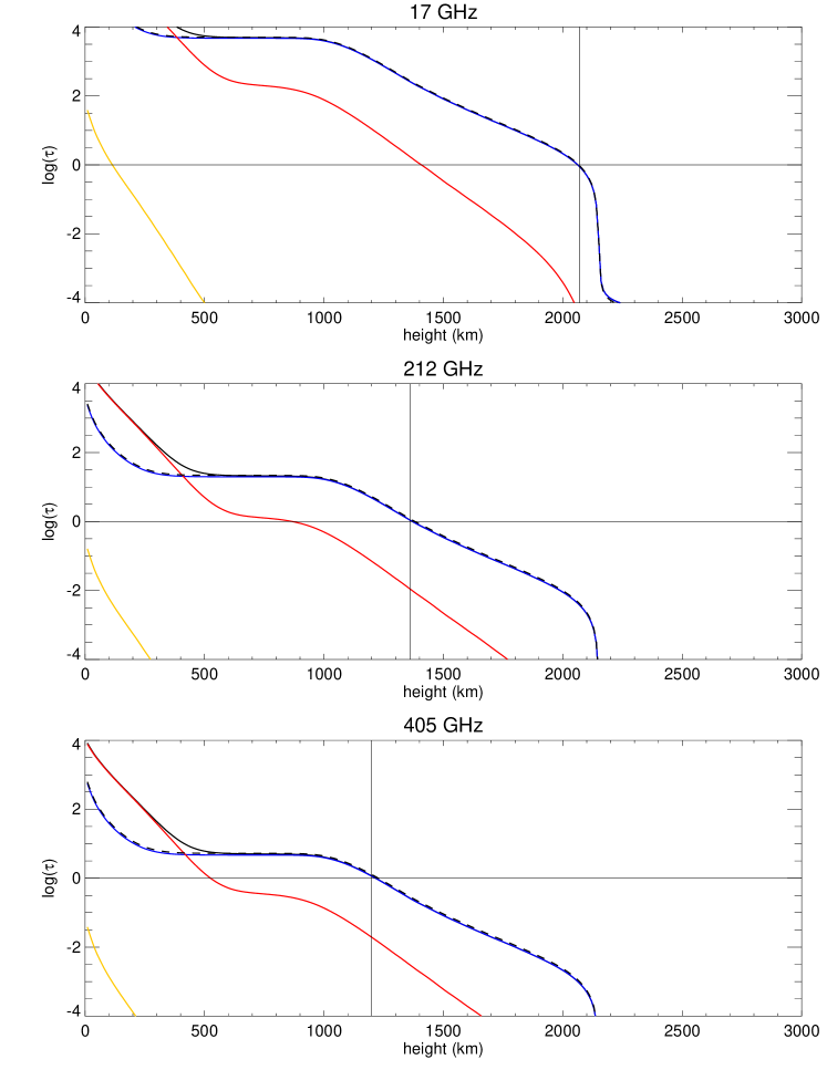
Figure 3: Optical Depth at 17, 212, and 405 GHz using the C07 input atmospheric model. In blue we show the contribution of the bremsstrahlung opacity, red $H^{-}$ and yellow the Inverse bremsstrahlung. The continuous line shows the sum of all the contributions and the dashed line represents only the bremsstrahlung opacity function.

Our code output gives us detailed information of the radiation parameters. As instance, in Figure 3 we show the computed optical depth at 17 (top), 212 (middle) and 405 (bottom) GHz as a function of radial height. We made two simulations, the first one using only bremsstrahlung opacity (dashed black lines); and the second one using our model Celestun, in this case, the yellow lines represent the inverse bremsstrahlung opacity; the $H^{-}$ opacity is shown by red lines; the blue lines correspond to the classical bremsstrahlung opacity; and the black continuous lines represent the full opacity function from Celestun. The introduction of $H^{-}$ and inverse bremsstrahlung opacities does not change the height where the atmosphere becomes optically thick ($\tau\sim 1$). However, it is clear that below 500 km, the $H^{-}$ process is the major source of opacity in the solar atmosphere.

The detailed local behavior of the emission at 17, 212 and 405 GHz is seen in Figure 4, where we have plotted the brightness temperature (black lines) and the input atmospheric radial temperature (yellow lines) as a function of the atmospheric height. The continuous and dashed lines represent, respectively, the cases where all, and only bremsstrahlung opacities were considered. The contribution, to the local brightness, of the absorption $\epsilon_{abs}$ (Eq. 16) is plotted in blue lines, whereas the emission $\epsilon_{emi}$ (Eq. 17) is plotted in red lines.

We note that there are two separated regions where clearly the emission has a significant contribution: the first one is close to the photosphere, and it is interesting to note that the height of this region increases when the $H^{-}$ opacity function is considered; The importance of the second enhanced emission region decreases with the frequency, and the $H^{-}$ opacity does not produce any differences in this region. The second enhanced region and the $H^{-}$ opacity do not affect the final brightness temperature, this is why these structures were unnoticed until now. The contribution of the inverse bremsstrahlung is negligible.

6 Synthetic Spectra

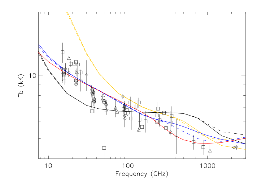
Figure 5: Synthetic solar spectra and observations at different stages of solar activity cycle, collected by Loukitcheva et al. (2004). The square points are intermediate, diamonds close-to-minimum, and triangles close-to-maximum of solar activity cycle. The solar spectra are shown for bremsstrahlung opacity (dashed line) and Celestun model (continuous line) for four input atmospheric models: C7 (black), SEL05 (blue), VALC (yellow) and SEL05 but using their electronic density (red).

It is interesting to compare the output of our code using different input atmospheric models. As instance, in Figure 5 we show observations performed at different phases of the solar cycle and collected by Loukitcheva et al. (2004): diamonds corresponds to close-to-minimum, the square symbols to intermediate, and triangles to close-to-maximum phases of the solar cycle. In the same figure, we have plotted the synthetic solar spectra computed using all (continuous lines) and only bremsstrahlung (dashed lines) opacities and the following input models: VALC in yellow lines; CAIUS05 (Selhorst et al., 2005) in blue lines; C7 in black lines; and again CAIUS05 but using their electronic density and physical assumptions (bremsstrahlung opacity and fully ionized atmosphere) in red lines.

There are interesting differences in the input atmospheric models, e.g., the altitude and the length of the chromospheric temperature minimum, as well as the altitude and the morphology of the chromospheric upper limit (i. e. the beginning of the transition zone and corona). The VALC model has the temperature minimum closer to the photosphere and is the warmest. This model has a thin chromosphere and defines a “plateau zone”, where the chromosphere temperature reach 20,000 K. This plateau is responsible of the high brightness temperature at low frequencies (see Figure 5 and de La Luz et al., 2008). The CAIUS05 model has similar altitude for the temperature minimum but is hotter and is shorter compared to the VALC model. The chromospheric temperature grows exponentially up to coronal values. The CAIUS05 model has the largest chromosphere. The C7 model has the lowest temperature minimum, and then a constant temperature until the rise due to the transition region and the corona. This model eliminates the plateau zone using ambipolar diffusion.

In order to facilitate the analysis, we consider separately three regions of the spectrum: from 2 to 60 GHz (low frequency); from 60 to 400 GHz (intermediate frequency); and from 400 GHz to 3 THz (high frequency).

At low frequency range, the temperature differences of the atmospheric models produce significant differences in the spectra (regardless of the opacity function), this emitting region is located at the upper chromosphere $\sim 1500$ km over the photosphere. For intermediate frequencies, the simulations agree rather well with the observations, however, the observations have large dispersion. Finally, at high frequency range we note that there is an apparent discontinuity at 400 GHz. In this region the model that better fits the observations is CAIUS05. On the other hand, both C07 and VALC models predict higher brightness temperatures than the observed.

These apparent minimal differences between input atmospheric models, produce significant differences in the resultant synthetic spectra computed from our radiative model.

7 Discussion and Conclusions

Using different atmospheric models and opacity functions, we have computed the optical depth, $\tau$, at low atmospheric altitudes. Our results show that if we use either, only bremsstrahlung or Celestun (i.e. $H$, $H^{-}$ and inverse Bremsstrahlung) opacities, the height over the photosphere where the overlying atmosphere becomes optically thick ($\tau\approx 1$) remains unalterable. However, if we take into account the local emissivity (Eq. 17) we show that the height where the main emission is generated, changes meaningfully.

For example, at 17 GHz the height over the photosphere where the atmosphere starts to become optically thin is around $1500$ km, but the height where $\tau=1$ is around $2050$ km. There are local emissivity structures below $1500$ km, although they remain invisible to the observer because the atmosphere is optically thick at these heights. When we considered bremsstrahlung opacity only, the local emissivity at 17 GHz changes in a region between $500$ and $850$ km over the photosphere (the atmosphere becomes optically thin). This structure is not present when the Celestun model is considered.

At 212 and 405 GHz the behavior of the local emissivity changes noticeably, since at these frequencies two regions of emissivity are present: A lower one, closer to the photosphere shows deep differences when comparing between both models. The height of the region where the emission is generated is higher by 200 km when the Celestun model is used. The uppermost region is located between $800$ and $1500$ km above the photosphere. In this region there is no difference between the two models. As seen in Figure 4, the second layer of emission is below the $\tau=1$ height and is similar for both models. Even more, after $1000$ km, the brightness temperature remains unalterable. This is due to the fact that the temperature of the atmospheric model is the upper limit for the brightness temperature, and remains constant between $1000$ and $2000$ km above the photosphere. the brightness temperature remains unalterable. These facts mask the local emission processes which are unnoticed by the observer.

We found that the dominant emission mechanism changes with altitude: $H^{-}$ is dominant below $500$ km whereas bremsstrahlung dominates at upper heights, although the final brightness temperature remains unchanged.

Our results show that the inclusion of the $H^{-}$ and inverse bremsstrahlung mechanisms does not modify the final brightness temperature. But the $H^{-}$ opacity function has a significant impact in the local emissivity and absorbency and it must be considered when studying micro structures in the low chromosphere. Therefore Celestun code is a valuable tool to perform this kind of studies. The inverse bremsstrahlung has no impact on the brightness temperature, neither on the local emissivity nor on the absorbency processes.

We note that there are more emission mechanisms acting at the low solar atmosphere, as instance, molecular emission has been reported for CO (Solanki et al., 1994) and also in the 515.60 to 516.20 nm spectral range ($C_{2}$ and $MgH$, Faurobert & Arnaud, 2002). The emitting layer has been situated below the $1100$ km, making evident that these molecules are present in a thin layer inside the temperature minimum region, between the photosphere and the low chromosphere. However, observations in visible wavelengths, have shown that the molecular emission at the limb brightening region is negligible, corresponding to 0.2% of the continuum intensity at the center of the solar disk. Nevertheless, a detailed study of the contribution of the molecular rotational spectrum at these wavelengths is necessary.

Although our simulations are related to quiescent solar situations, the next natural steps will be to investigate and compare with flaring cases. Therefore, such researches could in principle be used to better understand the thermal structure of the flaring solar atmosphere, that is the response of the atmosphere to flare energy release. From the few existing semi-empirical flare models like Machado et al. (1980) and Mauas et al. (1990) we should grossly expect decreasing radio fluxes as a function of increasing wavelengths in the range from centimeter to far-infrared wavelengths.

We will pay special attention to the density structure of the flaring loops (due to its importance in the computed opacity functions). It is clear that new simulations, observations and their comparison are needed to better investigate the structure and dynamics of the low layers of the solar atmosphere during flares.

Figure 1: Temperature vs Hydrogen density for VALC model (solid line) and C07 Model (dashed line) in the dynamic space.

Figure 2: Departure coefficients for VALC (dashed line) and C07 (continue line) approximated model taking into account the $b_{1}$ parameter published in the VALC model. We note that for both models $b_{1}$ parameter follow the radial temperature. The main differences are seen above 1500 km over the photosphere.

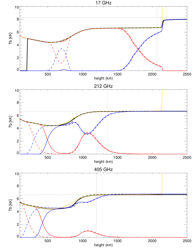
Figure 4: Local absorption ($\epsilon_{abs}$, blue) and local emissivity ($\epsilon_{emi}$, red) for 17, 212, and 405 GHz (top to bottom) using the C07 input atmospheric model. In yellow we show the radial temperature and in black the brightness temperature.

References

- Ahmad & Kundu (1981) Ahmad, I. A., & Kundu, M. R. 1981, Sol. Phys., 69, 273
- Alexander & Ferguson (1994) Alexander, D. R., & Ferguson, J. W. 1994, ApJ, 437, 879
- Athay & Thomas (1961) Athay, R. G., & Thomas, R. N. 1961, Physics of the solar chromosphere, ed. Athay, R. G. & Thomas, R. N.
- Avrett & Loeser (2008) Avrett, E. H., & Loeser, R. 2008, ApJS, 175, 229
- Ayres (1989) Ayres, T. R. 1989, Sol. Phys., 124, 15
- Brussaard & van de Hulst (1962) Brussaard, P. J., & van de Hulst, H. C. 1962, Reviews of Modern Physics, 34, 507
- Chiuderi & Chiuderi Drago (2004) Chiuderi, C., & Chiuderi Drago, F. 2004, A&A, 422, 331
- Chiuderi Drago et al. (1983) Chiuderi Drago, F., Kundu, M. R., & Schmahl, E. J. 1983, Sol. Phys., 85, 237
- Cillié & Menzel (1935) Cillié, G. G., & Menzel, D. H. 1935, Harvard College Observatory Circular, 410, 1
- de La Luz et al. (2008) de La Luz, V., Lara, A., Mendoza, E., & Shimojo, M. 2008, Geofisica Internacional, 47, 197
- De la Luz et al. (2010) De la Luz, V., Lara, A., Mendoza-Torres, J. E., & Selhorst, C. L. 2010, ApJS, 188, 437
- Dulk (1985) Dulk, G. A. 1985, ARA&A, 23, 169
- Faurobert & Arnaud (2002) Faurobert, M., & Arnaud, J. 2002, A&A, 382, L17
- Giovanelli (1949) Giovanelli, R. G. 1949, MNRAS, 109, 298
- Golovinskii & Zon (1980) Golovinskii, P. A., & Zon, B. A. 1980, Zhurnal Tekhnicheskoi Fiziki, 50, 1847
- John (1988) John, T. L. 1988, A&A, 193, 189
- Kaufmann et al. (2008) Kaufmann, P., Levato, H., Cassiano, M. M., Correia, E., Costa, J. E. R., Giménez de Castro, C. G., Godoy, R., Kingsley, R. K., Kingsley, J. S., Kudaka, A. S., Marcon, R., Martin, R., Marun, A., Melo, A. M., Pereyra, P., Raulin, J., Rose, T., Silva Valio, A., Walber, A., Wallace, P., Yakubovich, A., & Zakia, M. B. 2008, in Society of Photo-Optical Instrumentation Engineers (SPIE) Conference Series, Vol. 7012, Society of Photo-Optical Instrumentation Engineers (SPIE) Conference Series
- Kundu (1970) Kundu, M. R. 1970, Sol. Phys., 13, 348
- Kurucz (1979) Kurucz, R. L. 1979, ApJS, 40, 1
- Kuznetsova (1978) Kuznetsova, N. A. 1978, Soviet Astronomy, 22, 345
- Landi & Chiuderi Drago (2003) Landi, E., & Chiuderi Drago, F. 2003, ApJ, 589, 1054
- Loukitcheva et al. (2004) Loukitcheva, M., Solanki, S. K., Carlsson, M., & Stein, R. F. 2004, A&A, 419, 747
- Machado et al. (1980) Machado, M. E., Avrett, E. H., Vernazza, J. E., & Noyes, R. W. 1980, ApJ, 242, 336
- Mauas et al. (1990) Mauas, P. J. D., Machado, M. E., & Avrett, E. H. 1990, ApJ, 360, 715
- Menzel (1937) Menzel, D. H. 1937, ApJ, 85, 330
- Nakajima et al. (1995) Nakajima, H., Nishio, M., Enome, S., Shibasaki, K., Takano, T., Hanaoka, Y., Torii, C., Sekiguchi, H., Bushimata, T., Kawashima, S., Shinohara, N., Irimajiri, Y., Koshiishi, H., Kosugi, T., Shiomi, Y., Sawa, M., & Kai, K. 1995, Journal of Astrophysics and Astronomy Supplement, 16, 437
- Raulin & Pacini (2005) Raulin, J.-P., & Pacini, A. A. 2005, Advances in Space Research, 35, 739
- Rybicki & Lightman (1986) Rybicki, G. B., & Lightman, A. P. 1986, Radiative Processes in Astrophysics (Radiative Processes in Astrophysics, by George B. Rybicki, Alan P. Lightman, pp. 400. ISBN 0-471-82759-2. Wiley-VCH , June 1986.)
- Selhorst et al. (2005) Selhorst, C. L., Silva, A. V. R., & Costa, J. E. R. 2005, A&A, 433, 365
- Solanki et al. (1994) Solanki, S. K., Livingston, W., & Ayres, T. 1994, Science, 263, 64
- Sommerfeld & Maue (1935) Sommerfeld, A., & Maue, A. W. 1935, Annalen der Physik, 415, 589
- Vernazza et al. (1973) Vernazza, J. E., Avrett, E. H., & Loeser, R. 1973, ApJ, 184, 605
- Vernazza et al. (1976) —. 1976, ApJS, 30, 1
- Vernazza et al. (1981) —. 1981, ApJS, 45, 635
- Wildt (1939) Wildt, R. 1939, ApJ, 90, 611
- Zheleznyakov (1996) Zheleznyakov, V. V., ed. 1996, Astrophysics and Space Science Library, Vol. 204, Radiation in Astrophysical Plasmas