On the infeasibility of entanglement generation in Gaussian quantum systems via classical control

Abstract

This paper uses a system theoretic approach to show that classical linear time invariant controllers cannot generate steady state entanglement in a bipartite Gaussian quantum system which is initialized in a Gaussian state. The paper also shows that the use of classical linear controllers cannot generate entanglement in a finite time from a bipartite system initialized in a separable Gaussian state. The approach reveals connections between system theoretic concepts and the well known physical principle that local operations and classical communications cannot generate entangled states starting from separable states.

I Introduction

Entanglement is a unique feature of quantum mechanical systems not found in classical systems and is responsible for some of their predicted counterintuitive behavior, as exemplified by the famous Einstein-Podolsky-Rosen paradox [1]. Entanglement gives rise to experimentally verifiable non-classical correlations among measurement statistics [2] that cannot be explained by the usual classical probability models. One well known application of entanglement is quantum teleportation, the process of transferring the unknown state of one quantum system to another whilst destroying the state of the former, without the two quantum systems ever interacting directly with one another [3]. This process is at the heart of quantum communication schemes.

A bipartite quantum system is the composite of two quantum systems. The state of such a system will be referred to as a bipartite state and is represented by a density operator $\rho$. Suppose that the system is composed of a quantum system A with underlying Hilbert space $\mathcal{H}_{A}$ and a quantum system B with underlying Hilbert space $\mathcal{H}_{B}$. A state $\rho$ is said to be separable if it can be decomposed as $\rho=\sum_{k}p_{k}\rho^{A}_{k}\otimes\rho^{B}_{k}$, with $\rho_{k}^{A}$ and $\rho_{k}^{B}$ being density operators on $\mathcal{H}_{A}$ and $\mathcal{H}_{B}$, respectively, for $k=1,2,\ldots$. Here $\otimes$ denotes the tensor product of operators. If a bipartite state is not separable, then it is said to be entangled. For a pure state density operator $\rho$ (i.e., ${\rm tr}(\rho^{2})=1$), it can be easily determined if it is separable; e.g., see [4]. However, determining the separability of a mixed state bipartite density operator $\rho$ (i.e., ${\rm tr}(\rho^{2})<1$), is far from straightforward and a complete characterization is only known for certain types of bipartite systems, such as for bipartite systems on the finite dimensional Hilbert space $\mathbb{C}^{2}\otimes\mathbb{C}^{2}$. In fact, the general problem of determining the separability of a given mixed quantum state is known to be NP-hard [5]. Another class of bipartite systems for which a complete characterization of separability is known is the class of bipartite Gaussian systems [6, 7, 8, 9]. These systems are commonly encountered in the field of quantum optics. For such systems, the underlying Hilbert space is the tensor product of two quantum harmonic oscillator Hilbert spaces; e.g., see [10, Chapter III]. Also, the separability of a state can be completely determined from the (symmetrized) covariance matrix of the canonical position and momentum operators of the system [6]. The class of systems considered in this paper is the class of bipartite Gaussian systems. In particular, we analyze dynamical bipartite Gaussian quantum systems whose covariance matrices evolve in time. Hence, the separability or entanglement of these systems also evolves in time. In quantum optics, these dynamical bipartite Gaussian systems correspond to a class of linear quantum stochastic systems [11, 12, 13] that are driven by Gaussian bosonic fields and with a density operator initially in a Gaussian state. The dynamics of such systems can be represented by linear quantum stochastic differential equations (QSDEs) in the canonical position and momentum operators and this makes them suitable for a system-theoretic analysis.

We study the problem of entanglement generation using classical finite dimensional (linear time-invariant (LTI) and time varying) controllers from a system-theoretic point of view. The main contribution of the paper is the use of system theoretic arguments and methods to show that the application of a classical linear dynamic controller cannot induce entanglement in a dynamical bipartite Gaussian system which is initially in a separable state. Our result is in agreement with the fundamental physical principle that Local Operations and Classical Communication (LOCC) cannot generate entanglement between initially separable states; e.g., see [4] for a proof of this result. One motivation for the results of this paper is that they provide a starting point for investigating connections between systems theory and quantum physical principles. The no-go results for Gaussian quantum systems considered here are in a similar spirit to other no go results that have previously been obtained in [14], showing that linear modulation of a beam cannot create out-of-loop squeezing, and [15], showing that neither in-cavity squeezing nor output squeezing can be created using linear modulation of the cavity field.

II Preliminaries

II-A Notation

We will use the following notation: $\mathfrak{i}=\sqrt{-1}$, ^∗ denotes the adjoint of a linear operator as well as the conjugate of a complex number. If $A=[a_{jk}]$ then $A^{\#}=[a_{jk}^{*}]$, and $A^{{\dagger}}=(A^{\#})^{T}$, where ^T denotes matrix transposition. $\Re\{A\}=(A+A^{\#})/2$ and $\Im\{A\}=\frac{1}{2\mathfrak{i}}(A-A^{\#})$. We denote the identity matrix by $I$ whenever its size can be inferred from context and use $I_{n}$ to denote an $n\times n$ identity matrix. Similarly, $0$ denotes a matrix with zero entries whose dimensions can be determined from context. ${\rm diag}(M_{1},M_{2},\ldots,M_{n})$ denotes a block diagonal matrix with square matrices $M_{1},M_{2},\ldots,M_{n}$ on its diagonal, and ${\rm diag}_{n}(M)$ denotes a block diagonal matrix with the square matrix $M$ appearing on its diagonal blocks $n$ times. Also, we will let $J=\left[\begin{array}[]{rr}0&1\\ -1&0\end{array}\right]$.

II-B The class of linear quantum stochastic systems

In this paper, we are concerned with a class of quantum stochastic models of open (i.e., quantum systems that can interact with an environment) Markov quantum systems that are widely used in the area of quantum optics. Such models have been used in the physics and mathematical physics literature since at least the 1980’s; e.g., see [16, 17, 18, 19, 20]. We focus on the special sub-class of linear quantum stochastic models (e.g., see [21, Section 7.2], [20, Section 6.6], [19, Sections 3, 3.4.3, 5.3, Chapters 7 and 10], [22], [23, Section 5], [11, 12, 13, 24]) that describe the Heisenberg evolution of the (canonical) position and momentum operators of several independent open quantum harmonic oscillators that are coupled to external coherent bosonic fields, such as coherent laser beams. These linear stochastic models describe quantum optical devices such as optical cavities [25, Section 5.3.6][21, Chapter 7], linear quantum amplifiers [19, Chapter 7], and finite bandwidth squeezers [19, Chapter 10]. Following [11, 12, 13], we will refer to this class of models as linear quantum stochastic systems.

Suppose we have $n$ independent quantum harmonic oscillators. The $j$th quantum harmonic oscillator has position and momentum operators $q_{j}$ and $p_{j}$ with underlying Hilbert space $L^{2}(\mathbb{R})$; see, e.g., [10, Chapter III]. The position and momentum operators satisfy the canonical commutation relations $[q_{j},p_{k}]=2\mathfrak{i}\delta_{jk}$, $[q_{j},q_{k}]=0$, and $[p_{j},p_{k}]=0$, where $\delta_{jk}$ denotes the Kronecker delta and $[\cdot,\cdot]$ denotes the commutation operator. The quantum harmonic oscillators are assumed to be coupled to $m$ external independent quantum fields modelled by bosonic annihilation field operators $\mathcal{A}_{1}(t),\mathcal{A}_{2}(t),\ldots,\mathcal{A}_{m}(t)$ which are defined on separate Fock spaces (over $L^{2}(\mathbb{R})$) for each field operator [16, 18]. For each annihilation field operator $\mathcal{A}_{j}(t)$, there is a corresponding creation field operator $\mathcal{A}_{j}^{*}(t)$, which is defined on the same Fock space and is the operator adjoint of $\mathcal{A}_{j}(t)$. The field operators are adapted quantum stochastic processes with forward differentials $d\mathcal{A}_{j}(t)=\mathcal{A}_{j}(t+dt)-\mathcal{A}_{j}(t)$ and $d\mathcal{A}_{j}^{*}(t)=\mathcal{A}_{j}^{*}(t+dt)-\mathcal{A}_{j}^{*}(t)$ that have the quantum Itô products [16, 18]: $d\mathcal{A}_{j}(t)d\mathcal{A}_{k}(t)^{*}=\delta_{jk}dt;\,d\mathcal{A}_{j}^{*}(t)d\mathcal{A}_{k}(t)=d\mathcal{A}_{j}(t)d\mathcal{A}_{k}(t)=d\mathcal{A}_{j}^{*}(t)d\mathcal{A}_{k}^{*}(t)=0.$

We collect the position and momentum operators in the column vector $x$ defined by $x=(q_{1},p_{1},q_{2},p_{2},\ldots,q_{n},p_{n})^{T}$. Note that we may write the canonical commutation relations as $xx^{T}-(xx^{T})^{T}=2\mathfrak{i}\Theta$ with $\Theta={\rm diag}_{n}(J)$. We take the composite system of $n$ quantum harmonic oscillators to have a quadratic Hamiltonian $H$ given by $H=\frac{1}{2}x^{T}Rx$, where $R$ is a real $2n\times 2n$ symmetric matrix. The quantum harmonic oscillators are coupled to the $k$-th quantum field via the singular interaction Hamiltonian $H_{k}=\mathfrak{i}(L_{k}\eta_{k}^{*}(t)-L_{k}^{*}\eta_{k}(t))$ [17, 19], where $L_{k}=K_{k}x$ (with $K_{k}\in\mathbb{C}^{1\times 2n}$) is a linear coupling operator describing the linear coupling of the quantum harmonic oscillator position and momentum operators to $\eta_{k}(t)$. Here $\eta_{k}(t)$ is a quantum white noise process [17, 19] satisfying the relation $\mathcal{A}_{k}(t)=\int_{0}^{t}\eta_{k}(s)ds$. We now collect the coupling operators $L_{1},L_{2},\ldots,L_{m}$ together in one linear coupling vector $L=(L_{1},L_{2},\ldots,L_{m})^{T}=Kx$, with $K=[\begin{array}[]{cccc}K_{1}^{T}&K_{2}^{T}&\ldots&K_{m}^{T}\end{array}]^{T}$, and collect the field operators together as $\mathcal{A}(t)=(\mathcal{A}_{1}(t),\mathcal{A}_{2}(t),\ldots,\mathcal{A}_{m}(t))^{T}$. Then the joint evolution of the oscillators and the quantum fields is given by a unitary adapted process $U(t)$ satisfying the Hudson-Parthasarathy QSDE [16, 18]:

$$dU(t) = \biggl{(}{\rm tr}\bigl{(}(S-I)^{T}d\Lambda(t)\bigr{)}+d\mathcal{A}(t)^{{\dagger}}L-L^{{\dagger}}Sd\mathcal{A}(t)$$

$$\quad-(\mathfrak{i}H+\frac{1}{2}L^{{\dagger}}L)dt\biggr{)}U(t),$$

where $S\in\mathbb{C}^{m\times m}$ is a complex unitary matrix (i.e., $S^{{\dagger}}S=SS^{{\dagger}}=I$) called the scattering matrix, and $\Lambda(t)=[\Lambda_{jk}(t)]_{j,k=1,\ldots,m}$, with $\Lambda_{kj}(t)=\Lambda_{jk}(t)^{*}$. The processes $\Lambda_{jk}(t)$ for $j,k=1,\ldots,m$ are adapted quantum stochastic processes referred to as gauge processes, and the forward differentials $d\Lambda_{jk}(t)=\Lambda_{jk}(t+dt)-\Lambda_{jk}(t)$ $j,k=1,\ldots,m$ have the quantum Itô products:

$$d\Lambda_{jk}(t)d\Lambda_{j^{\prime}k^{\prime}}(t) = \delta_{kj^{\prime}}d\Lambda_{jk^{\prime}}(t),\ d\mathcal{A}_{j}(t)d\Lambda_{kl}(t)=\delta_{jk}d\mathcal{A}_{l}(t),$$

$$d\Lambda_{jk}d\mathcal{A}_{l}(t)^{*} = \delta_{kl}d\mathcal{A}_{j}^{*}(t),$$

with all other remaining cross products between $\mathcal{A}_{j}(t),\mathcal{A}^{*}_{k}(t),\Lambda_{j^{\prime}k^{\prime}}(t)$ being $0$.

For any adapted processes $X(t)$ and $Y(t)$ satisfying a quantum Itô stochastic differential equation, we have the quantum Itô rule $d(X(t)Y(t))=X(t)dY(t)+(dX(t))Y(t)+dX(t)dY(t)$; e.g., see [16, 18]. Using the quantum Itô rule and the quantum Itô products given above, as well as exploiting the canonical commutation relations between the operators in $x$, the Heisenberg evolution $x(t)=U(t)^{*}xU(t)$ of the canonical operators in the vector $x$ can be obtained. Then $x(t)$ satisfies the QSDE (see [22, 23, 11, 13]):

$$dx(t) =d(U(t)^{*}xU(t)),$$

$$=A_{o}x(t)dt+B_{o}\left[\small\begin{array}[]{c}d\mathcal{A}(t)\\ d\mathcal{A}(t)^{\#}\end{array}\normalsize\right];x(0)=x,$$ (3)

$$dY(t) =d(U(t)^{*}\mathcal{A}(t)U(t)),$$

$$=C_{o}x(t)dt+D_{o}d\mathcal{A}(t),$$ (4)

with $A_{o}=2\Theta(R+\Im\{K^{{\dagger}}K\})$, $B_{o}=2\mathfrak{i}\Theta[\begin{array}[]{cc}-K^{{\dagger}}S&K^{T}S^{\#}\end{array}]$, $C_{o}=K$, and $D_{o}=S$. Here, $Y(t)=(Y_{1}(t),\ldots,Y_{m}(t))^{T}=U(t)^{*}\mathcal{A}(t)U(t)$ is a vector of output fields that results from the interaction of the quantum harmonic oscillators and the incoming quantum fields $\mathcal{A}(t)$. Note that the dynamics of $x(t)$ is linear, and $Y(t)$ depends linearly on $x(t)$. We refer to $n$ as the number of degrees of freedom of the linear quantum stochastic system.

In this paper it will be convenient to write the dynamics in quadrature form as in [11]:

$$dx(t) =Ax(t)dt+Bdw(t);\,x(0)=x.$$

$$dy(t) =Cx(t)dt+Ddw(t),$$ (5)

with

$$w(t) = 2(\Re\{\mathcal{A}_{1}(t)\},\Im\{\mathcal{A}_{1}(t)\},\ldots,\Re\{\mathcal{A}_{m}(t)\},\Im\{\mathcal{A}_{m}(t)\})^{T};$$

$$y(t) = 2(\Re\{Y_{1}(t)\},\Im\{Y_{1}(t)\},\ldots,\Re\{Y_{m}(t)\},\Im\{Y_{m}(t)\})^{T}.$$

Here, the real matrices $A,B,C,D$ are in a one to one correspondence with the matrices $A_{o},B_{o},C_{o},D_{o}$. Also, the quantity $w(t)$ satisfies the Itô relationship $dw(t)dw(t)^{T}=F_{w}dt$ where $F_{w}\geq 0$; see [11]. Furthermore, we define the matrix $S_{w}=\frac{1}{2}\left(F_{w}+F_{w}^{\#}\right)$ and the differential commutation matrix $T_{w}=\frac{1}{2}\left(F_{w}-F_{w}^{\#}\right)$. For the boson fields that we consider here, $T_{w}$ is necessarily of the form $T_{w}=\mathfrak{i}{\rm diag}_{m}(J)$. The symmetric matrix $S_{w}$ is then such that $F_{w}\geq 0$ and for the Gaussian boson fields that are of interest here this matrix reflects the statistics of the field. For instance, $S_{w}=I$ corresponds to a vacuum Gaussian boson field.

Fig. 1 shows an example of a two degree of freedom linear quantum stochastic system connected to a classical controller. The linear quantum stochastic system consists of two independent optical cavities [25, 21, 13] denoted by $G_{1}$ and $G_{2}$. The two optical cavities are connected to the classical controller via a homodyne detector (HD) which measures one of the quadratures of the output field $Y_{1}(t)$ from $G_{1}$, and an electro-optic modulator (MOD) which modulates the quantum field $\mathcal{A}_{3}(t)$ with the controller output signal $u(t)$ and then sends the resulting field $\mathcal{A}_{2}(t)$ to $G_{2}$.

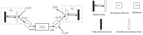
Figure 1: The interconnection of two optical cavities $G_{1}$ and $G_{2}$ via a classical controller.

Remark 1

For the remainder of this paper, we will consider the case where $n=2$, corresponding to two degree of freedom linear quantum stochastic systems, with the quantum harmonic oscillators being initialized in a Gaussian state. Also, for such a linear quantum stochastic system $G$, we define a (linear) dynamical bipartite Gaussian quantum system (corresponding to $G$) as the open quantum system obtained from $G$ by tracing out (averaging) the bosonic fields.

III Simple system-theoretic proof of the Heisenberg Uncertainty Principle

For a system of the form (5), the corresponding symmetric covariance matrix defined by

$$P(t)=\frac{1}{2}{\rm tr}(\rho(0)(x(t)x(t)^{T}+(x(t)x(t)^{T})^{T}))$$

varies with time. Here, $\rho(0)$ is the initial density operator of the overall composite closed system. In this section, we will assume that the matrix $A$ in (5) is Hurwitz. Then the steady-state symmetrized covariance matrix $P=\mathop{\lim}_{t\rightarrow\infty}P(t)$ satisfies the real Lyapunov equation (see, e.g., [20, p. 327], [12, Section 4]):

$$AP+PA^{T}+BS_{w}B^{T}=0.$$ (6)

On the other hand, since the commutation relations are preserved, we also have that [11]:

$$A\Theta+\Theta A^{T}-\mathfrak{i}BT_{w}B^{T}=0.$$ (7)

Defining the complex Hermitian matrix $\tilde{P}=P+\mathfrak{i}\Theta$, we see from combining (6) and (7) that $\tilde{P}$ satisfies the complex Lyapunov equation: $A\tilde{P}+\tilde{P}A^{T}+BF_{w}B^{T}=0$, where $F_{w}=S_{w}+T_{w}$. Since $F_{w}\geq 0$ and $A$ is Hurwitz, it follows that $\tilde{P}\geq 0$; e.g., see [27]. Equivalently, in terms of $P$ and $\Theta$ we have that: $P+\mathfrak{i}\Theta\geq 0$. This matrix inequality is a version of the Heisenberg Uncertainty Principle that must be satisfied by all Gaussian quantum systems; e.g., see [6, 7] for this alternate form of the Heisenberg Uncertainty Principle.

IV Classical LTI controllers cannot generate steady-state bipartite entanglement in linear Gaussian quantum systems

IV-A Separability criterion for dynamical bipartite Gaussian systems

It has been shown in [6] that the separability of a bipartite Gaussian density operator $\rho$ can be completely determined from a complex linear matrix inequality (LMI) involving the (symmetrized) covariance matrix $P=\frac{1}{2}{\rm tr}(\rho(xx^{T}+(xx^{T})^{T}))$; see also [8, 9].

Lemma 2 ([6, 8, 9])

A bipartite Gaussian density operator $\rho$ is separable if and only if the corresponding covariance matrix $P$ satisfies the LMI $P+\mathfrak{i}{\rm diag}(J,-J)\geq 0$.

Note here that without loss of generality, we can assume that $x$ has zero mean because the mean of $x$ plays no role in determining the separability of the associated density operator. Now, in the case of a dynamical bipartite Gaussian quantum system corresponding to a linear quantum stochastic system, the covariance matrix can vary with time and is given by

$$P(t) = \frac{1}{2}{\rm tr}(\rho_{\rm o}(t)(xx^{T}+(xx^{T})^{T}))$$ (8)

$$= \frac{1}{2}{\rm tr}(\rho(t)(xx^{T}+(xx^{T})^{T}))$$

$$= \frac{1}{2}{\rm tr}(\rho(0)(x(t)x(t)^{T}+(x(t)x(t)^{T})^{T})),$$

where $\rho(t)$ is the density operator at time $t\geq 0$ of the overall composite closed system, while $\rho_{\rm o}(t)$ is the reduced density operator of the two quantum harmonic oscillators at time $t$ obtained by tracing out the bosonic fields; e.g., see [19]. Note that the second equality in (8) follows from the definition of the partial trace (e.g., see [18, p. 102]) since the elements of $x$ are operators on the bipartite quantum harmonic oscillator Hilbert space. Also, the final equality in (8) follows by switching from the Schrödinger picture (in which $\rho(t)$ evolves in time) to the Heisenberg picture (in which $x(t)$ evolves in time and the overall density operator is fixed as $\rho(0)$). Thus, to check whether the system is separable at any time $t\geq 0$, it is equivalent to check if the LMI $P(t)+\mathfrak{i}{\rm diag}(J,-J)\geq 0$ is satisfied at that time $t$.

IV-B Separability of dynamical bipartite Gaussian systems coupled via a classical LTI controller

Let $G_{1}=(A_{1},B_{1},C_{1},D_{1})$ and $G_{2}=(A_{2},B_{2},C_{2},D_{2})$ define two linear quantum stochastic systems of the form (5). We form a linear quantum stochastic system $G=(A,B,C,D)$ of the form (5) from $G_{1}$ and $G_{2}$, with $A={\rm diag}(A_{1},A_{2})$, $B={\rm diag}(B_{1},B_{2})$, $C={\rm diag}(C_{1},C_{2})$, and $D={\rm diag}(D_{1},D_{2})$. We then obtain a dynamical bipartite Gaussian quantum system corresponding to $G$ (see Remark 1). The quantum system $G$ is connected to a finite dimensional classical controller as shown in Fig. 2 to form a quantum feedback control system. In this quantum feedback control system, some of the output fields from $G_{1}$ and $G_{2}$ are measured and fed to the classical controller that processes these measurements linearly to produce control signals that are fed back into $G_{1}$ and/or $G_{2}$. Here, control actuation can be facilitated in two ways:

1. Modulating the Hamiltonian of $G_{k}$ by a classical $2\times 1$ signal vector $u_{1,k}$. If the canonical operators of $G_{k}$ are represented by a vector of operators $x_{k}=(q_{k},p_{k})^{T}$, this means that the quadratic Hamiltonian $H_{k}$ of $G_{k}$ is augmented by adding a linear (time varying) Hamiltonian term $H_{l,k}(t)$ of the form $H_{l,k}(t)=u_{1,k}(t)^{T}M_{k}x_{k}$, where $M_{k}$ is a real $2\times 2$ matrix. Thus, the total Hamiltonian for $G_{k}$ becomes $H_{k}+H_{l,k}(t)$. The signal $u_{1,k}(t)$ is classical and can depend linearly on the classical controller internal variables (i.e., its state) as well as the measurement results. This actuation can be implemented in different ways, for instance, as described in the Appendix of [28].

2. Modulating (or displacing) an input field of $G_{k}$ with a classical control signal $u_{2,k}(t)$. This can be implemented by an electro-optic modulator.

In the quantum feedback control system shown in Fig. 2, the vector of quantum input fields $\mathcal{A}_{k}(t)$ for the system $G_{k}$ is partitioned into two parts: some of which will be the components of $\mathcal{A}_{k1}(t)$ while the others will be components of $\mathcal{A}_{k2}(t)$. Here $\mathcal{A}_{k1}(t)$ represents the input fields of $G_{k}$ that will not be modulated by the controller, while $\mathcal{A}_{k2}(t)$ represents the input fields that are modulated by the controller. Part of the output vector of quantum signals, $Y_{k2}(t)$, of $G_{k}$ ($k=1,2$) is passed through a network of static optical components (as listed in [13, Section 6.2]) and homodyne detectors (labelled as HDN in the diagram) that produces the set of classical measurements signals $m_{k}(t)$ which drive the controller. The controller produces two sets of classical control signals ($k=1,2$): one set, $u_{k1}(t)$, modulates the linear Hamiltonian term $H_{1,k}$, and another set, $u_{k2}(t)$, is modulated by a network of (possibly electro-optic) modulators (denoted in the diagram by MOD) to produce the quantum signal $\mathcal{A}_{k2}(t)$ as one of the input fields into $G_{k}$. The signals $\mathcal{V}_{jk}(t)$, $j,k=1,2$ are any additional quantum noises required for the operation of HDN and MOD (they may be suitably absorbed into the definition of $w_{1}$ or $w_{2}$).

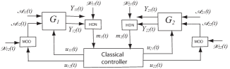
Figure 2: Interconnection of $G_{1}$ and $G_{2}$ via a classical controller.

The assumptions that we will use regarding this quantum feedback control system are:

1. The control $u(t)=(u_{1,1}(t),u_{2,1}(t),u_{1,2}(t),u_{2,2}(t))^{T}$ has been generated by a finite dimensional linear (time invariant or time varying) system.

2. The quantum signals coming into $G_{1}$ and $G_{2}$ come from independent sources. Therefore, $F_{w}={\rm diag}(F_{w_{1}},F_{w_{2}})$ and hence, $S_{w}={\rm diag}(S_{w_{1}},S_{w_{2}})$, $T_{w}={\rm diag}(T_{w_{1}},T_{w_{2}})$.

Note that the systems $G_{1}$ and $G_{2}$ are not directly connected to one another. That is, no output field from $G_{1}$ is passed directly to $G_{2}$ and vice-versa. They are only indirectly connected via the classical controller. Note also that the overall closed-loop system is then a mixed classical-quantum linear stochastic system as described in [11].

Let $z(t)$ denote the controller internal state which is classical in nature and of arbitrary dimension $n_{c}$. We could also allow the classical controller to be driven by an additional classical Wiener noise source $w_{c}(t)$ that is not derived from the measurement signals. However, this additional noise may be absorbed into $w_{1}$ or $w_{2}$; see [11] for details. Now, let $x(t)=(x_{1}(t),x_{2}(t),z(t))^{T}$ and $w(t)=(w_{1}(t),w_{2}(t))^{T}$ where $x_{1}(t)$ represents the vector of system variables for the quantum system $G_{1}$ and $w_{1}(t)$ represents the vector of quantum noise inputs for $G_{1}$. Also, $x_{2}(t)$ represents the vector of system variables for the quantum system $G_{2}$ and $w_{2}(t)$ represents the vector of quantum noise inputs for $G_{2}$. Now, since $G_{1}$ and $G_{2}$ each only interact with the controller, it follows that the dynamics of the closed-loop system can be written in the form:

$$dx(t) = \tilde{A}x(t)dt+\tilde{B}dw(t);x(0)=x,$$ (9)

where the real matrices $\tilde{A}$ and $\tilde{B}$ have the special structure:

$$\tilde{A} = \left[\small\begin{array}[]{ccc}A_{11}&0&A_{13}\\ 0&A_{22}&A_{23}\\ A_{31}&A_{32}&A_{33}\end{array}\normalsize\right];\quad\tilde{B}=\left[\small\begin{array}[]{cc}B_{11}&0\\ 0&B_{22}\\ B_{31}&B_{32}\end{array}\normalsize\right],$$

with $A_{11}=A_{1},\,A_{22}=A_{2}\,,B_{11}=B_{1};\,B_{22}=B_{2}$. Our main result in this section is the following.

Theorem 3

Consider any classical LTI controller that is connected to the linear quantum system $G$ such that $\tilde{A}$ is Hurwitz in the closed loop system (9). Then the resulting closed-loop dynamical bipartite Gaussian quantum system is separable at steady state. Thus, a classical LTI controller cannot generate an entangled steady state from any initial Gaussian state.

Proof:

Since the controller state $z(t)$ is classical, the commutation matrix $\Theta$ for $x(t)$ will be degenerate canonical [11, Sections II, III, and III C] of the form $\Theta=\left[\small\begin{array}[]{ccc}\Theta_{1}&0&0\\ 0&\Theta_{2}&0\\ 0_{n_{c}\times 2}&0_{n_{c}\times 2}&0_{n_{c}\times n_{c}}\end{array}\normalsize\right],$ where $\Theta_{1}=\Theta_{2}=J$. Suppose that the controller state $z(t)$ is of arbitrary dimension $n_{c}$. We have that the closed-loop mixed quantum-classical system satisfies the constraint [11, Theorem 3.4] : $\tilde{A}\Theta+\Theta\tilde{A}^{T}-\mathfrak{i}\tilde{B}T_{w}\tilde{B}^{T}=0,$ with $T_{w}={\rm diag}(T_{w_{1}},T_{w_{2}})$. This equation is equivalent to the following:

$$\left[\small\begin{array}[]{cc}A_{11}\Theta_{1}+\Theta_{1}A_{11}^{T}-\mathfrak{i}B_{11}T_{w_{1}}B_{11}^{T}\\ 0\\ A_{31}\Theta_{1}-\mathfrak{i}B_{31}T_{w_{1}}B_{11}^{T}\end{array}\normalsize\right.$$ (14)

$$\quad\small\begin{array}[]{c}0\\ A_{22}\Theta_{2}+\Theta_{2}A_{22}^{T}-\mathfrak{i}B_{22}T_{w_{2}}B_{22}^{T}\\ A_{32}\Theta_{2}-\mathfrak{i}B_{32}T_{w_{2}}B_{22}^{T}\end{array}\normalsize$$ (18)

$$\quad\left.\small\begin{array}[]{c}\Theta_{1}A_{31}^{T}-\mathfrak{i}B_{11}T_{w_{1}}B_{31}^{T}\\ \Theta_{2}A_{32}^{T}-\mathfrak{i}B_{22}T_{w_{2}}B_{32}^{T}\\ -\mathfrak{i}B_{32}T_{w_{2}}B_{32}^{T}\end{array}\normalsize\right]=0.$$ (22)

(23)

Multiplying the $(2,2)$, $(2,3)$, $(3,2)$, and $(3,3)$ elements of this matrix equation by $-1$, yields

$$\left[\small\begin{array}[]{c}A_{11}\Theta_{1}+\Theta_{1}A_{11}^{T}-\mathfrak{i}B_{11}T_{w_{1}}B_{11}^{T}\\ 0\\ A_{31}\Theta_{1}-\mathfrak{i}B_{31}T_{w_{1}}B_{11}^{T}\end{array}\normalsize\right.$$ (27)

$$\quad\small\begin{array}[]{cc}0\\ -A_{22}\Theta_{2}-\Theta_{2}A_{22}^{T}+\mathfrak{i}B_{22}T_{w_{2}}B_{22}^{T}\\ -A_{32}\Theta_{2}+\mathfrak{i}B_{32}T_{w_{2}}B_{22}^{T}\end{array}\normalsize$$ (31)

$$\quad\left.\small\begin{array}[]{c}\Theta_{1}A_{31}^{T}-\mathfrak{i}B_{11}T_{w_{1}}B_{31}^{T}\\ -\Theta_{2}A_{32}^{T}+\mathfrak{i}B_{22}T_{w_{2}}B_{32}^{T}\\ \mathfrak{i}B_{32}T_{w_{2}}B_{32}^{T}\end{array}\normalsize\right]=0.$$ (35)

Letting $\hat{\Theta}={\rm diag}(\Theta_{1},-\Theta_{2},0_{n_{c}\times n_{c}})$ and $\hat{T}_{w}={\rm diag}(T_{w_{1}},-T_{w_{2}})$, this matrix equality can be written as: $\tilde{A}\hat{\Theta}+\hat{\Theta}\tilde{A}^{T}-\mathfrak{i}\tilde{B}\hat{T}_{w}\tilde{B}^{T}=0.$ We now use the fact that the closed-loop matrix $\tilde{A}$ is Hurwitz. Then, as discussed in Section III, the symmetrized steady state covariance matrix $P$ satisfies: $\tilde{A}P+P\tilde{A}^{T}+\tilde{B}S_{w}\tilde{B}^{T}=0.$ Defining $\tilde{P}=P+\mathfrak{i}\hat{\Theta}$ and $\tilde{F}_{w}=S_{w}+\hat{T}_{w}$, we have that $\tilde{P}$ satisfies the complex Lyapunov equation: $\tilde{A}\tilde{P}+\tilde{P}\tilde{A}^{T}+\tilde{B}\tilde{F}_{w}\tilde{B}^{T}=0.$ Recalling that $S_{w}={\rm diag}(S_{w_{1}},S_{w_{2}})$ and $F_{w}\geq 0$, we note that $F_{w_{i}}=S_{w_{i}}+T_{w_{i}}\geq 0$ for $i=1,2$. Then, we note that since $\tilde{F}_{w}={\rm diag}(F_{w_{1}},F_{w_{2}}^{\#})$, we have that $\tilde{F}_{w}\geq 0$; see, e.g., [27]. Therefore, since $\tilde{A}$ is Hurwitz, we have that $\tilde{P}\geq 0$. Partitioning $P$ according to the partitioning of $x(t)$ into its quantum and classical components as $P=\left[\small\begin{array}[]{cc}P_{11}&P_{12}\\ P_{21}&P_{22}\end{array}\normalsize\right]$, the property $\tilde{P}=P+\mathfrak{i}\hat{\Theta}\geq 0$ implies that $P_{11}+\mathfrak{i}{\rm diag}(\Theta_{1},-\Theta_{2})=P_{11}+\mathfrak{i}{\rm diag}(J,-J)\geq 0.$ Therefore it follows from Lemma 2 that the dynamical bipartite Gaussian quantum system is separable at steady-state. Thus, a classical LTI controller cannot generate an entangled steady state from any initial Gaussian state. ∎

Removing the classical controller by defining all its system matrices to be zero, a special case of Theorem 3 shows that two independent and unconnected systems $G_{1}$ and $G_{2}$, with $A_{1}$ and $A_{2}$ Hurwitz, which are initially entangled become separable in the steady state.

V Classical finite dimensional linear controllers cannot generate any entanglement in bipartite Gaussian quantum systems in finite time

In the previous section, we have shown that starting from any state, separable or entangled, a classical LTI controller cannot generate or maintain entanglement at steady state in a linear dynamical bipartite Gaussian quantum system. In this section, by a slight modification of the arguments of the previous section, we will show that classical finite dimensional linear controllers cannot generate bipartite entanglement in a finite time for any initially separable linear dynamical bipartite Gaussian quantum system. Moreover, for this finite time analysis, we may drop the requirement that the controller is chosen so that the closed-loop matrix $\tilde{A}$ is Hurwitz.

We follow the notation and set up of the last section. Instead of considering the steady state covariance matrix $P$, we now consider the symmetrized finite time covariance matrix $P(t)=\frac{1}{2}{\rm tr}\bigl{(}\rho(0)(x(t)x(t)^{T}+(x(t)x(t)^{T})^{T})\bigr{)}$, $0\leq t<\infty$ satisfying the Lyapunov differential equation:

$$\dot{P}(t) = \tilde{A}P(t)+P(t)\tilde{A}^{T}+\tilde{B}S_{w}\tilde{B}^{T},\quad P(0)=P_{0}.$$

Theorem 4

Suppose that a linear dynamical bipartite Gaussian quantum system is initially separable. Then it remains separable for all $t\geq 0$ under the action of any classical LTI controller.

Proof:

Since the system is initially separable, $P(0)+\mathfrak{i}\hat{\Theta}\geq 0$ by Lemma 2. Let $\tilde{P}(t)=P(t)+\mathfrak{i}\hat{\Theta}$. Then following the same lines of argument as in the proof of Theorem 3, and by using standard results on Lyapunov differential equations, we find that since $\tilde{P}(0)\geq 0$ and $\tilde{F}_{w}\geq 0$ (hence also $\tilde{B}\tilde{F}_{w}\tilde{B}^{T}\geq 0$) that $\tilde{P}(t)\geq 0,$ for all $t\geq 0$ regardless of the values of $\tilde{A}$ and $\tilde{B}$. Similarly partitioning $P(t)$ according to the partitioning of $x(t)$ into its quantum and classical components as $P(t)=\left[\small\begin{array}[]{cc}P_{11}(t)&P_{12}(t)\\ P_{12}(t)&P_{22}(t)\end{array}\normalsize\right]$, it follows that $P_{11}(t)+\mathfrak{i}{\rm diag}(J,-J)\geq 0,$ for all $t\geq 0$. This shows that when the bipartite Gaussian system is initially in a separable state, then under the action of a classical LTI controller it will remain so for all times. ∎

Remark 5

Note that it is straightforward to extend the proof of the above theorem to allow for linear time-varying controllers rather than LTI controllers.

Example 6

Consider the quantum optical system shown in Fig. 1. Suppose that the two optical cavities are identical with the partially reflecting mirror on each cavity having coupling coefficient $0.01$. Also, let the position and momentum operators of cavity $G_{i}$ be $(q_{i},p_{i})$, and let $\tilde{x}=(q_{2},p_{2},q_{1},p_{1})^{T}$. Let $w_{i1}(t)=2\Re\{\mathcal{A}_{i}(t)\}$ and $w_{i2}(t)=2\Im\{\mathcal{A}_{i}(t)\}$, $i=1,2,3$. Then the dynamics of the two degree of freedom linear quantum stochastic system (without the controller, homodyne detector and modulator attached) is given by:

$$d\tilde{x}(t) =-0.005\tilde{x}(t)dt-0.1d(w_{21}(t),w_{22}(t),w_{11}(t),w_{12}(t))^{T},$$

$$dy^{o}(t) =0.1\tilde{x}(t)dt+d(w_{21}(t),w_{22}(t),w_{11}(t),w_{12}(t))^{T}.$$

Let $y^{o}(t)=(y^{o}_{1}(t),y^{o}_{2}(t),y^{o}_{3}(t),y^{o}_{4}(t))^{T}$. The amplitude quadrature $y^{o}_{3}(t)$ of $y^{o}(t)$ is measured using the homodyne detector and is used as the (stochastic) input $m_{1}(t)=y^{o}_{3}(t)$ to a first order LTI controller that produces a two dimensional output signal $u(t)=(u_{1}(t),u_{2}(t))^{T}$. The dynamics of the controller is:

$$dz(t) =Az(t)dt+Bdm_{1}(t),\;z(0)=0,$$

$$u(t) =\left[\begin{array}[]{cc}C_{1}^{T}&C_{2}^{T}\end{array}\right]^{T}z(t),$$

where $z(t)$ denotes the state of the controller, and $A=-1$, $B=C_{1}=C_{2}=1$. The output signal $u(t)$ is passed through an electro-optic modulator and sent to the partially reflecting mirror of cavity $G_{2}$. Let $x(t)=(\tilde{x}(t),z(t))^{T}$. We then have that the interconnection of the controller with the two cavities via the homodyne detector and electro-optic modulator is a mixed quantum-classical system with dynamics of the form (9) defined by the matrices

$$\tilde{A} =\left[\small\begin{array}[]{ccccc}-0.005&0&0&0&-0.1C_{1}\\ 0&-0.005&0&0&-0.1C_{2}\\ 0&0&-0.005&0&0\\ 0&0&0&-0.005&0\\ 0&0&0.1B&0&A\end{array}\normalsize\right];$$

$$\tilde{B} =\left[\small\begin{array}[]{cccc}-0.1&0&0&0\\ 0&-0.1&0&0\\ 0&0&-0.1&0\\ 0&0&0&-0.1\\ 0&0&B&0\end{array}\normalsize\right],$$

and is driven by the noise $(w_{31}(t),w_{32}(t),w_{11}(t),w_{12}(t))^{T}$. Suppose that the bipartite state of the two cavities is in an initially entangled bipartite Gaussian state with covariance matrix $P_{11}(0)$ given below in (36)

$$P_{11}(0)=\left[\small\begin{array}[]{cccc}0.5028&0&-0.0528&0\\ 0&0.5028&0&0.0528\\ -0.0528&0&0.5028&0\\ 0&0.0528&0&0.5028\end{array}\normalsize\right].$$ (36)

We take as our measure of entanglement the logarithmic negativity $E_{N}$ [29, 4, 28]. Partitioning $P_{11}(t)$ into $2\times 2$ blocks as $\left[\small\begin{array}[]{cc}P_{11,1}(t)&P_{11,2}(t)\\ P_{11,2}(t)^{T}&P_{11,3}(t)\normalsize\end{array}\right]$, $E_{N}(P_{11}(t))$ is given by $E_{N}(P_{11}(t))=\max(0,-\ln(2\nu(t)))$, where $\nu(t)=\frac{1}{\sqrt{2}}\sqrt{\tilde{\Delta}(t)-\sqrt{\tilde{\Delta}(t)^{2}-4\det(P_{11}(t))}}$ and $\tilde{\Delta}(t)=\det(P_{11,1}(t))+\det(P_{11,3}(t))-2\det(P_{11,2}(t))$. Note that the logarithmic negativity is always nonnegative and has a value of zero if and only if the state is separable [29, 4], otherwise the state is entangled, with a higher value of $E_{N}$ indicating a higher degree of entanglement. The initial value of the logarithmic negativity is $E_{N}(P_{11}(0))=0.1054$. The solid line in Fig. 3 shows that under the action of this classical controller, the logarithmic negativity steadily decreases and finally goes to zero in a finite time. At this point, the state becomes separable and remains so for all future times. If we instead start at an initially separable state with covariance matrix $P_{11}(0)$ as given in (37)

$$P_{11}(0)=\left[\small\begin{array}[]{cccc}0.5704&0&0.0034&0.0562\\ 0&0.5704&0&0.0528\\ 0.0034&0&0.6203&0.0499\\ 0.0562&0.0528&0.0499&0.6203\end{array}\normalsize\right],$$ (37)

then the oscillators’ joint state remains separable, as shown in the dashed line in Fig. 3.

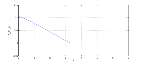
Figure 3: The evolution of logarithmic negativity $E_{N}(P_{11}(t))$ over time for the system considered in Example 6. The solid line shows the evolution starting from an entangled state with covariance matrix $P_{11}(0)$ in (36). The dashed line shows the evolution starting from a separable state with covariance matrix $P_{11}(0)$ in (37).

VI Conclusions

By employing system-theoretic arguments and methods, we were able to give a systems theory proof of the fact that classical LTI controllers cannot generate steady state entanglement in linear dynamical bipartite Gaussian quantum systems. Furthermore, we also give a systems theory proof of the fact that classical linear controllers cannot generate entanglement in a dynamical bipartite Gaussian system initially in a separable state. An interesting topic for future research is to consider system-theoretic analysis of entanglement between the continuous-mode output fields.

References

- [1] M. Nielsen and I. Chuang, Quantum Computation and Quantum Information. Cambridge: Cambridge University Press, 2000.
- [2] A. Aspect, P. Grangier, and G. Roger, “Experimental realization of Einstein-Podolsky-Rosen-Bohm gedankenexperiment: A new violation of Bell’s inequalities,” Phys. Rev. Lett., vol. 49, no. 2, pp. 91–94, 1982.
- [3] B. Bennett, G. Brassard, C. Crépeau, R. Jozsa, A. Peres, and W. K. Wootters, “Teleporting an unknown quantum state via dual classical and Einstein-Podolsky-Rosen channels,” Phys. Rev. Lett., vol. 70, no. 13, pp. 1895–1899, March 1993.
- [4] M. Plenio and S. Virmani, “An introduction to entanglement measures,” Quantum Inf. Comput., vol. 7, pp. 1–51, 2007.
- [5] L. Gurvits, “Classical complexity and quantum entanglement,” Journal of Computer and System Sciences, vol. 69, no. 3, pp. 448–484, 2004.
- [6] R. Simon, “Peres-Horodecki separability criterion for continuous variable systems,” Phys. Rev. Lett., vol. 84, no. 12, pp. 2726–2729, 2000.
- [7] A. S. Holevo, “Some statistical problems for quantum Gaussian states,” IEEE Trans. Inform. Theory, vol. 21, no. 5, pp. 533–543, 1975.
- [8] G. Adesso, “Entanglement of Gaussian states,” Ph.D. dissertation, University of Salerno, 2007.
- [9] S. Pirandola, A. Serafini, and S. Lloyd, “Correlation matrices of two-mode bosonic systems,” Phys. Rev. A, vol. 79, pp. 052 327–2–052 327–10, 2009.
- [10] P. A. Meyer, Quantum Probability for Probabilists, 2nd ed. Berlin-Heidelberg: Springer-Verlag, 1995.
- [11] M. R. James, H. I. Nurdin, and I. R. Petersen, “ control of linear quantum stochastic systems,” IEEE Trans. Automat. Contr., vol. 53, no. 8, pp. 1787–1803, 2008.
- [12] H. I. Nurdin, M. R. James, and I. R. Petersen, “Coherent quantum LQG control,” Automatica J. IFAC, vol. 45, pp. 1837–1846, 2009.
- [13] H. I. Nurdin, M. R. James, and A. C. Doherty, “Network synthesis of linear dynamical quantum stochastic systems,” SIAM J. Control Optim., vol. 48, no. 4, pp. 2686–2718, 2009.
- [14] J. Shapiro, G. Saplakoglu, S.-T. Ho, P. Kumar, B. Saleh, and M. Teich, “Theory of light detection in the presence of feedback,” J. Opt. Soc. Am. B, vol. 4, no. 10, pp. 1604–1620, October 1987.
- [15] H. Wiseman and G. Milburn, “Squeezing via feedback,” Phys. Rev. A, vol. 49, no. 2, pp. 1350–1366, 1994.
- [16] R. L. Hudson and K. R. Parthasarathy, “Quantum Ito’s formula and stochastic evolution,” Commun. Math. Phys., vol. 93, pp. 301–323, 1984.
- [17] C. W. Gardiner and M. J. Collett, “Input and output in damped quantum systems: Quantum stochastic differential equations and the master equation,” Phys. Rev. A, vol. 31, no. 6, pp. 3761 – 3774, 1985.
- [18] K. Parthasarathy, An Introduction to Quantum Stochastic Calculus. Berlin: Birkhauser, 1992.
- [19] C. Gardiner and P. Zoller, Quantum Noise: A Handbook of Markovian and Non-Markovian Quantum Stochastic Methods with Applications to Quantum Optics, 2nd ed., ser. Springer Series in Synergetics. Springer, 2000.
- [20] H. M. Wiseman and G. J. Milburn, Quantum Measurement and Control. Cambridge University Press, 2010.
- [21] D. F. Walls and G. Milburn, Quantum Optics. Berlin and Heidelberg: Springer-Verlag, 1994.
- [22] S. C. Edwards and V. P. Belavkin, “Optimal quantum filtering and quantum feedback control,” August 2005, University of Nottingham. [Online]. Available: http://arxiv.org/pdf/quant-ph/0506018.
- [23] V. P. Belavkin and S. C. Edwards, “Quantum filtering and optimal control,” in Quantum Stochastics and Information: Statistics, Filtering and Control (University of Nottingham, UK, 15 - 22 July 2006), V. P. Belavkin and M. Guta, Eds. Singapore: World Scientific, 2008, pp. 143–205.
- [24] H. Mabuchi, “Coherent-feedback quantum control with a dynamic compensator,” Phys. Rev. A, vol. 78, pp. 032 323–1–032 323–5, 2008.
- [25] H. Bachor and T. Ralph, A Guide to Experiments in Quantum Optics, 2nd ed. Weinheim, Germany: Wiley-VCH, 2004.
- [26] G. Linblad, “Brownian motion of harmonic oscillators: Existence of a subdynamics,” J. Math. Phys., vol. 39, no. 5, pp. 2763–2780, 1998.
- [27] D. S. Bernstein, Matrix Mathematics: Theory, Facts, And Formulas with Application to Linear Systems Theory. Princeton, New Jersey: Princeton University Press, 2005.
- [28] N. Yamamoto, H. I. Nurdin, M. R. James, and I. R. Petersen, “Avoiding entanglement sudden death via measurement feedback control in a quantum network,” Phys. Rev. A, vol. 78, pp. 042 339–1 – 042 339–11, 2008.
- [29] G. Vidal and R. F. Werner, “Computable measure of entanglement,” Phys. Rev. A, vol. 65, no. 3, p. 032314, 2002.