Black holes and the absorption rate of cosmological scalar fields

Abstract

We study the absorption of a massless scalar field by a static black hole. Using the continuity equation that arises from the Klein-Gordon equation, it is possible to define a normalized absorption rate $\Gamma(t)$ for the scalar field as it falls into the black hole. It is found that the absorption mainly depends upon the characteristics wavelengths involved in the physical system: the mean wavenumber and the width of the wave packet, but that it is insensitive to the scalar field’s strength. By taking a limiting procedure, we determine the minimum absorption fraction of the scalar field’s mass by the black hole, which is around $50\%$.

I Introduction

Black holes, a concept that emerged from the simplest exact solution of Einstein’s equations, are some of the most fascinating objects in gravitational physics. Equally fascinating is our current belief that most galaxies must host a supermassive black hole (SMBH) in their center, with mass values in the range of $10^{5}$ to $10^{10}$ solar masses, most likely in a state of very low matter accretion nowadaysCaramete and Biermann (2011); *Volonteri:2011rm; *Ferrarese:2002ct; *Nowak:2007ba; *Greenwood:2005cs; Ghez et al. (2000). In particular, the measurements of the velocities of stars near the center of the Milky Way have provided strong evidence for the presence of a SBH with a mass of around $4\times 10^{6}M_{\odot}$Ghez et al. (2000).

There are some models that attempt to explain the present existence of galactic SMBH’s. Among others, we can mention the collision of two or more black holes to form a larger one, the core-collapse of a stellar cluster, and the formation of primordial black holes directly out from the primordial plasma in the first instants of time after the Big BangMelia (2007); *Carr:2009jm.

The key point in the discussion are the features of the precise mechanism under which a black hole can accrete enough matter to become supermassive. In particular, some authors have proposed that primordial black holes (PBH) can go supermassive simply by accreting matter from a cosmological scalar field related to dark energy (quintessence). In a first study, the authors inBean and Magueijo (2002) (see alsoBabichev et al. (2004); *Babichev:2005py; Mersini-Houghton and Kelleher (2008); Rodrigues and Saa (2009)) found that PBH could have effectively accreted enough matter from a quintessence field endowed with an exponential potential.

The calculations for the accretion were in fact based upon the simple and exact results of the accretion of a massless scalar field into a black hole found inJacobson (1999), see alsoFrolov and Kofman (2003); Harada and Carr (2005); Rodrigues and Saa (2009). However, the results inBean and Magueijo (2002) were later refused inCustodio and Horvath (2005), where was shown that the quintessence flux must decrease slower than $t^{-2}$ for PBHs to grow at all. This same result seems to have been confirmed by other authors under more general assumptionsFrolov and Kofman (2003); Harada and Carr (2005); Carr et al. (2010).

On the other hand, a related topic is the use of a cosmological scalar field as model for dark matter in the UniverseSahni and Wang (2000); *Matos:2000ng; *Matos:2000ss; *Arbey:2001qi; *Matos:2008ag; *Arbey:2006it; *Liddle:2006qz, and the possibility that they can be the dominant matter in galaxy halosSin (1994); *Ji:1994xh; *Arbey:2003sj; *Alcubierre:2003sx; *Guzman:2003kt; *Matos:2007zza; *Bernal:2009zy; *Barranco:2010ib; *UrenaLopez:2010ur. If so, then one has to address the accretion of this dark matter scalar field into the central SBH that seems to be present in most galaxiesUrena-Lopez and Liddle (2002); Cruz-Osorio et al. (2011).

The aim of this paper is to present some simple results of the interaction of a scalar field with a black hole, with numerical calculations based upon previous works in the literatureMarsa and Choptuik (1996); *Thornburg:1998cx; *Choptuik:2003 that may be useful in the understanding of the accretion, in general terms, of cosmological scalar fields into black holes.

We shall make use of the fact that there exists a continuity equation of the scalar field as long as the background spacetime is staticCho (2003). This fact will allow us to quantify the absorption rate of a scalar wave packet by a black hole in a more precise manner in terms of absorption flux and decay rates. For simplicity, we will only focus our attention in the case of a massless scalar field.

A brief summary of the paper is as follows. In Sec. II we set the mathematical background for the equations of motion, boundary conditions, and initial conditions for the scalar field’s wave packet. Here we also show the existence of a continuity equation arising directly from the equation of motion of the scalar field. In Sec. III, we present the main numerical results, and the description of the fall of the scalar field in terms of a normalized absorption rate. The latter arises naturally from the use of the continuity equation found in Sec. II. Finally, Sec. IV is devoted to conclusions and final comments.

II Mathematical background

We first consider a fixed Schwarzschild background with an Eddintong-Finkelstein (EF) gauge, which is defined such that $t+r$ is an ingoing null coordinate. Using the $3+1$ decomposition of the metricAlcubierre (2008); Thornburg (1999), the $3$-metric $\gamma_{ij}$ is

$$\gamma_{ij}=\mathrm{diag}\left[a^{2}(r),r^{2},r^{2}\sin^{2}\theta\right]\,,$$ (1)

where $a^{2}(r)=1+2GM/r$, $G$ is Newton’s constant, and $M$ denotes the mass of the black hole. The lapse $\alpha$ and shift $\beta^{i}=[\beta,0,0]$ functions are, respectively,

$$\alpha(r)=a^{-1}(r)\,,\quad\beta(r)=\frac{2GM}{a^{2}(r)r}\,.$$ (2)

It is illustrative to calculate the coordinate velocities of null geodesics, that are given by

$$\frac{dr}{dt}=c_{\pm}\equiv-\beta\pm\alpha/a\,.$$ (3)

Notice that the use of the EF gauge, from Eqs. (2), is manifest through the condition $c_{-}=-1$ for all points in the background spacetime (we use units in which $c=1$).

The Klein-Gordon (KG) equation for a massless self-interacting scalar field $\phi$ is

$$\frac{1}{\sqrt{-g}}\partial_{\mu}\left(\sqrt{-g}g^{\mu\nu}\partial_{\nu}\phi\right)=0\,.$$ (4)

In order to solve it, it proves convenient to define two first order variablesThornburg (1999); Alcubierre et al. (2003),

$$\Pi(t,r)=\partial_{r}\phi\,,\quad\eta(t,r)=\frac{1}{\alpha}\left(\partial_{t}\phi-\beta\Pi\right)\,,$$ (5)

with the help of which Eq. (4) is represented by the following three first order equations

$$\frac{1}{\alpha}\left(\partial_{t}\phi-\beta\partial_{r}\phi\right) = \eta\,,$$ (6a)

$$\frac{1}{\alpha}\left(\partial_{t}\Pi-\beta\partial_{r}\Pi\right) = \partial_{r}\eta+\frac{\beta}{2r}\eta+\partial_{r}\beta\,\Pi\,,$$ (6b)

$$\frac{1}{\alpha}\left(\partial_{t}\eta-\beta\partial_{r}\eta\right) = \frac{\partial_{r}\Pi}{a^{2}}+\frac{a^{2}+1}{r}\frac{\Pi}{a^{4}}+K\eta\,,$$ (6c)

where $K$ is the trace of the extrinsic curvature. Eq. (6a) arises from the very definition of $\eta$ and $\Pi$, whereas the equation for $\Pi$, Eq. (6b), arises from the combination of Eqs. (5); that of $\eta$ in Eq. (6c) arises from the original KG equation (4).

We shall take the quantity $(GM)$ as the unit for distance and time, so that the radial and time coordinates are made dimensionless through the change $r\to(GM)\hat{r}$ and $t\to(GM)\hat{t}$, where a hat denotes dimensionless variables. Notice that the unit for distance and time is half the usual Schwarzschild radius, $r_{S}\equiv 2GM$. The scalar field is made dimensionless by the change $\phi\to\hat{\phi}/\sqrt{G}$. Accordingly, the rest of the scalar field variables should be changed by the expressions $\Pi\to(m^{3}_{Pl}/M)\hat{\Pi}$, and $\eta\to(m^{3}_{Pl}/M)\hat{\eta}$, where the Planck mass is defined as $m^{2}_{Pl}=G^{-1}$.

We will impose outgoing-radiation boundary condition upon our field variables at the outermost points of the numerical grid. As for the innermost points, as long as they are inside the event horizon, there is no need to put a boundary condition, because the light cones there point inwards in the EF gauge, that is, $c_{+}<0$ and $c_{-}=-1$, see Eqs. (2), and (3).

The initial data for the scalar field in our numerical experiments will be a Gaussian profile modulated by a spherical wave of the form

$$\hat{\phi}(r)=A\frac{\cos{(\hat{k}_{0}\hat{r})}}{\hat{r}}e^{-\left(\hat{r}-\hat{r}_{0}\right)^{2}/\hat{\sigma}^{2}}\,,$$ (7)

which is centered at $\hat{r}=\hat{r}_{0}$, and has amplitude $A$ and width $\hat{\sigma}$. The Gaussian distribution of wavenumbers in Fourier space has a mean value $\langle\hat{k}\rangle=\hat{k}_{0}$, and variance $\langle(\hat{k}-\hat{k}_{0})^{2}\rangle=1/\hat{\sigma}^{2}$. It should be noticed here that the wave number was made dimensionless by the change $k\to\hat{k}/(GM)$.

On the other hand, by means of a lengthly but otherwise straightforward calculation, it can be shown that the KG equation (4) can be written in the form of a continuity equationCho (2003)

$$\partial_{t}\hat{\rho}-\frac{1}{\hat{r}^{2}}\partial_{\hat{r}}\left(\hat{r}^{2}\hat{J}^{r}\right)=0\,,$$ (8)

where the charge density $\hat{\rho}$ and the scalar field current density $\hat{J}^{r}$ are, respectively,

$$\hat{\rho} = \frac{1}{2}\left(\hat{\eta}^{2}+\frac{\hat{\Pi}^{2}}{a^{2}}\right)+\frac{\beta}{\alpha}\hat{\Pi}\hat{\eta}\,,$$ (9a)

$$\hat{J}^{r} = \beta\left(\hat{\eta}^{2}+\alpha^{2}\hat{\Pi}^{2}\right)+\alpha\left(\alpha^{2}+a^{2}\beta^{2}\right)\hat{\Pi}\,\hat{\eta}\,.$$ (9b)

In what follows, we will skip the hats of the variables, in the understanding that they have been made dimensionless. We may use a hat again on the variables whenever confusion may arise.

III Numerical results

The massless scalar field corresponds exactly to the solution of the (homegeneous) wave equation in a curved spacetime. One important feature of the massless case, which is helpful for the study of wave packets, is that the field keeps its shape as it falls into the black hole. Heuristically, this can be seen from the fact that the phase $v_{p}$ and group $v_{g}$ velocities of the wave packet are both equal to that of light, $v_{p}=v_{g}=c_{\pm}$. For illustration purposes, this nice feature can be seen directly in the motion of the wave packets shown in Fig. 1.

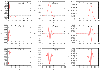
Figure 1: Motion of a Gaussian packet for different values of its mean wavenumber $k_{0}$, see Eq. (7). The wave packets retain their shape as they approach the black hole’s horizon, located at $r=2$. The wave packets were given ingoing initial conditions, $\eta=\Pi$. The time in each row proceeds from right to left.

We are solving differential equations with a finite differencing method, which involves the truncation of a Taylor series expansion. It is then necessary to show the proper convergence of numerical output as the spatial grid is refined. In Fig. 2, we show numerical runs with three different resolutions, where $R_{1}$ has coarse resolution, $R_{2}$ has medium resolution, and $R_{3}$ is the finest. As expected, the runs show that the numerical code is second order convergent.

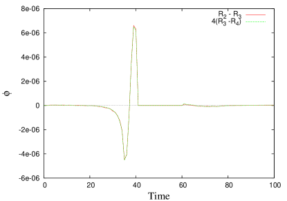
Figure 2: Convergence plot for the numerical code used to solve the KG equation in a fixed Schwarzschild background. The example corresponds to the maximum of the wave function $\phi_{max}$ at each time in the simplest case $k_{0}=0$ (see also Fig. 1). Shown are three different runs with resolutions $R_{1}$: $\Delta r=0.025$, $R_{2}$: $\Delta r=0.0125$, and $R_{3}$: $\Delta r=0.00625$. The plots, after the indicated scaling, agree in their profile, then the numerical output is second order convergent.

To study the rate at which the a scalar field wave packet is absorbed by the black hole, we rely on the continuity equation. Notice that Eq. (8) looks pretty much the same as a typical conservation equation in flat spacetime. Taking a bounded proper volume $V$, we find

$$\partial_{t}\int_{V}\sqrt{-g}\,\rho\,dr\,d\Omega=\partial_{t}\int_{V}4\pi r^{2}\,\rho\,dr=4\pi\left.(r^{2}J^{r})\right|^{r_{2}}_{r_{1}}\,.$$ (10)

Under the assumption that the scalar field current decays rapidly enough as $r_{2}\to\infty$, we find the useful result

$$\frac{1}{M_{\phi}}\frac{dM_{\phi}}{dt}=-\frac{4\pi}{M_{\phi}}\left.(r^{2}J^{r})\right|_{r_{S}}=-\Gamma(t)\,,$$ (11)

where $M_{\phi}=4\pi\int_{V}r^{2}\,\rho\,dr$ is the total scalar field mass contained in the proper volume $V$. In fact, $M_{\phi}$ is the conserved charge of the field as suggested by the continuity equation (8). We can monitor the absorption rate of the (total) mass of the wave packet by calculating the scalar field current going through the inner surface; in our case, the inner radius is the black hole’s horizon, $r_{1}=r_{S}$.

Following standard notation in Physics, we have denoted the decay rate of the wave packet’s mass as $\Gamma(t)$, whose units are given in terms of $(GM)^{-1}$. In our case, this decay rate is just the normalized flux at the horizon of the black hole, being the normalization factor the total mass of the wave packet that still remains outside the black hole’s horizon.

Typical curves for the decay rate are shown in Fig. 3. An interesting and unexpected result is that the (normalized) decay rate $\Gamma(t)$ does not depend on the Gaussian’s amplitude $A$, that is, it does not depend on the field’s strength. This means that larger packets are absorbed at the same rate as are smaller packets. We can notice though that the mean wavenumber has an effect on the absorption, as the latter increases for larger values of $k_{0}$.

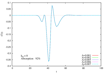
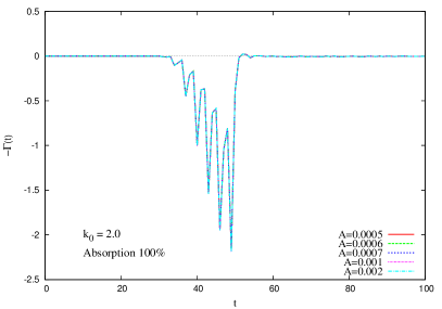
Figure 3: The (normalized) decay rate $\Gamma(t)$, see Eq. (11), of a massless scalar field $\phi$ as it flows through the black hole’s horizon. The units are given in terms of $(GM)^{-1}$, which for a typical mass of $10^{6}M_{\odot}$ gives $\Gamma\sim 0.2\mathrm{s}^{-1}$. The runs were performed for different values of the amplitude $A$ and of the mean wavenumber $k_{0}$ of the wave packet (7), whereas the width was fixed to $\sigma=5$. The total interaction time between the black hole and the wave packet is around $t_{T}\simeq 4\sigma$ in the two cases. The decay rate increases for larger values of $k_{0}$, but it is insensitive to the values of the amplitude $A$, i.e., to values of the scalar field’s strength.

If we integrate Eq. (11), we can find the total mass outside the horizon as a function of time,

$$\frac{M_{\phi}(t)}{M_{\phi,i}}=\exp\left(-\int\Gamma(t)dt\right)=\exp\left(-\Delta(t)\right)\,,$$ (12)

where $M_{\phi,i}$ is the initial total mass, and $\Delta(t)$ is the (exponential) absorption ratio. If the integral is calculated for the total time the wave packet is interacting with the black hole, it should give us the total absorption ratio of the wave packet. For the cases shown in Fig. 3, we have found that absorption is about $92\%$ for $k_{0}=0$, and $100\%$ for $k_{0}=2$. As a matter of fact, our numerical experiments showed that total absorption is always achieved if $k_{0}\geq r^{-1}_{S}$ (see alsoHernandez et al. (2009)).

As a final step, we study the dependence of $\Delta$ on the width of the wave packet; for definiteness, we focus our attention in the case $k_{0}=0$, which is also the most dispersive one. Numerical results are shown in Fig. 4, and we notice that the absorption decreases as the wave packet becomes wider. It can be verified that the points can be fitted by a function of the form

$$\Delta(\sigma)=e_{0}e^{-e_{1}\sigma}+e_{2}\,,$$ (13)

where, in the present case, a fitting procedure shows that $e_{0}=4.98$, $e_{1}=0.259$, and $e_{2}=0.67$. In particular, if wave packets as wide as necessary were allowed, then Eq. (13) suggests that the total absorption would be

$$\lim_{\sigma\to\infty}\Delta(\sigma)=0.67\,.$$ (14)

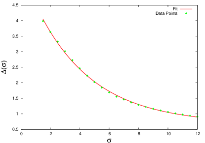
Figure 4: Total absorption ratio $\Delta$, see Eq. (12), for different widths of the wave packets; for all runs $k_{0}=0$. The amplitude $A$ was adjust in each case as to have always the same total mass $M_{\phi}$ at the initial time. This is not strictly necessary, as the decay rate is independent of the packet’s amplitude. We also show the fitting function (13).

IV Conclusions

The motion of a wave packet in a black hole spacetime raised some interest in the cosmological community because of the possibility that SMBH could have grown because of the accretion a Quintessence-type scalar field. This is not the only possible case, but we can ask the same question about any other cosmological scalar field living around a black hole.

We have explored the simplest possibility, that of a massless scalar field, for the motion of a wave packet in a fixed black hole spacetime using an EF gauge. To have a better visualization of the absorption of the scalar field by the black hole, we took advantage of the fact that one can write out a continuity equation from the KG equation.

The corresponding conserved charge is the total mass of the wave packet, but more important is the definition of a current density, with the help of which we were able to define a (normalized) decay rate for the wave packet, whose magnitude is given by the black hole’s mass, $\Gamma(t)\sim(GM)^{-1}$. This means that less massive black holes accrete scalar field matter at a larger rate; for example, a black hole as massive as the Sun would accrete at an incredible rate of $\Gamma\sim 10^{5}\mathrm{s}^{-1}$! In terms of the decay rate, we too found that the absorption depends on the mean wavenumber of the wave packet; actually, full absorption is reached for mean wavelengths smaller than the Schwarzschild radius, $k_{0}<r^{-1}_{S}$.

However, a new result showed up: the decay rate does not depend on the scalar field’s strength. Moreover, we could use this result to show the dependence of the absorption on the packet’s width. By a limiting procedure on a fitting function, we determined the maximum total absorption of a wave packet with a width much larger than the black hole’s horizon: around $e^{-0.67}\simeq 0.51$. This is the result that may have relevance for cosmology, as we expect cosmological scalar fields to have very large intrinsic length scales ($k_{0}\to 0$ and $\sigma\to\infty$) as compared to the Schwarzschild radius of supermassive black holes.

In the massless case studied here, there were two length scales involved: the mean wavelength $\lambda_{0}=k^{-1}_{0}$, and the width of the wave packet $\sigma$. We were able to show the general dependence of the (normalized) absorption rate on these length scales. In general, we can say that black holes are quite efficient in absorbing scalar fields, even in the case of very wide packets.

The method outlined here can be extended to the massive case. However, in the case the scalar field has a mass $m$, additional length scales appears in the problem in the form of the Compton length of the field, $\lambda_{C}\equiv m^{-1}$ and the Schwarzschild radius $r_{S}$ (in the massless case, the Schwarzschild radius does not appear explicitly in the equations of motion) that may introduce non-trivial features in the motion of the wave packet and its absorption rate. This is ongoing research that we expect to report elsewhere.