Probing mechanical quantum coherence with an ultracold-atom meter

Abstract

We propose a scheme to probe quantum coherence in the state of a nano-cantilever based on its magnetic coupling (mediated by a magnetic tip) with a spinor Bose Einstein condensate (BEC). By mapping the BEC into a rotor, its coupling with the cantilever results in a gyroscopic motion whose properties depend on the state of the cantilever: the dynamics of one of the components of the rotor angular momentum turns out to be strictly related to the presence of quantum coherence in the state of the cantilever. We also suggest a detection scheme relying on Faraday rotation, which produces only a very small back-action on the BEC and it is thus suitable for a continuous detection of the cantilever’s dynamics.

Recently, a considerable research effort has been put in achieving quantum control of micro and nano-scale mechanical systems espe . The role played by such objects in the current quest for demonstrating quantumness at the mesoscopic scale has changed in time, and by today they have become key players. Micro and nano-mechanical devices are now considered for quantum technological purposes as well as foundational questions espe ; cool ; cool2 .

As interesting and promising as they could be, such systems are in general very difficult to probe and measure directly. The necessity of isolating their fragile dynamics from the influences of the outside world and the need for low operating temperatures that allow for the magnification of the quantum mechanical features of their motion often imply that no direct access to such devices is possible. By today several schemes exist that use the interaction with light to extract information from the mechanical structures mauro . However, such methods are certainly not exhaustive and a more systematic approach to measure the quantum features of micro/nano-mechanical devices is highly desirable.

In this sense, a considerable step forward has been the design of interfaces between mechanical systems and ancillae such as superconducting systems and (ultra-)cold atomic ensembles tip ; mauro2 , which can be used to efficiently monitor, measure, and prepare the inaccessible mechanical counterparts. Most interestingly, some of these hybridization strategies are already mature enough to have found interesting preliminary implementations hunger . In this work we present a new strategy by demonstrating that the interaction between an ultra-cold atomic system and a mechanical oscillator can be exploited for effective diagnostics of mechanical quantum coherences. A similar approach has been used in a recent work kind for different purposes. Along the lines of Ref. tip , where it was shown that a similar system can mimic the strong coupling regime of cavity quantum electrodynamics, we consider a setup composed of a mechanical oscillator placed on an atom chip and coupled to a spinor BEC through a magnetic tip. In our scheme, the magnetic tip acts as a transducer turning the mechanical oscillations into a magnetic field experienced by the atomic spins. The motion of the latter in turn results in a driving force for the mechanical oscillator. A physically transparent description of the mechanism underlying our proposal is provided by the formal mapping of the spinor BEC onto a tridimensional rotor: the magnetic-like coupling between the atoms of the BEC and the mechanical system results in the interaction between a harmonic oscillator and one of the components of the rotor. This allows to “write” information of the coherences present in the cantilever state onto the state of the rotor, which can then be read out using a technique based on the optical Faraday effect. Our work provides a fully analytical framework for the proposed protocol and discusses a number of relevant cases showing the effectiveness of the scheme. The complexity of the problem, which requires the management of a very large sector of the Hilbert space of the cantilever-BEC system, demands the development of appropriate methods to include the relevant sources of noise affecting the device. A detailed treatment of this issue is left to future work.

The remainder of this work is organized as follows. In Sec. I and II we introduce the setup, the magnetic-like interaction Hamiltonian and, following Refs. spinorham ; mapping ; rotor , carefully guide through the formal mapping of the BEC onto a rotor. We finally recast the BEC-cantilever coupling terms into the form of a direct interaction between a harmonic oscillator and one of the components of the BEC rotor. In Sec. II.2 we propose a possible detection scheme by means of the read out of such a rotor component and apply our framework to a few relevant instances. In Sec. III we present our conclusions and briefly discusses a few interesting open questions.

I The set up and the Hamiltonian

We consider the setup sketched in Fig. 1, which consists of an on-chip single-clamped cantilever and a spinor BEC trapped in close proximity to the chip and the cantilever. The latter is assumed to be manufactured so as to accommodate at its free-standing end a single-domain magnetic molecule (or tip). Technical details on the fabrication methods of similar devices can be found in Refs. tip ; hunger , which have also been found to have very large quality factors, which guarantee a good resolution of the rich variety of modes in the cantilever’s spectrum. At room temperature, thermal fluctuations are able to (incoherently) excite all flexural and torsional modes and in the following we assume that a filtering process is put in place, restricting our observation to a narrow frequency window, so as to select only a single mechanical mode.

The second key element of our setup is a BEC of ⁸⁷Rb atoms held in an (tight) optical trap and prepared in the hyperfine level $|F=1\rangle$. As we assume the trapping to be optical, there is no distinction between atoms with different quantum numbers $m_{F}=0,\pm 1$ of the projections of the total spin along the quantization axis. Moreover, for a moderate number of atoms in the condensate and a tight trap, we can invoke the so-called single-mode approximation (SMA) SMAfail , which amounts to considering the same spatial distribution for all spin states. These approximations will be made rigorous and formal in the next Subsections.

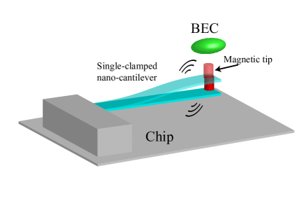
Figure 1: (Color online) Sketch of the set-up for BEC-based probing of mechanical coherences. A BEC is placed in close proximity to a nano-mechanical cantilever endowed with a magnetic tip. The coupling between the magnetic field generated by the mechanical quantum antenna and the ultra-cold atoms embodies a mechanism for the effective probing of coherences in the state of the mechanical system.

I.1 Hamiltonian of the system

In the following we will briefly review the mapping of a spinor BEC into a rotor rotor . The Hamiltonian of a BEC in second quantization reads spinorham

$$\hat{H} =\!\!\sum_{\alpha}\int d{\bf x}\hat{\Psi}_{\alpha}^{\dagger}({\bf x})\hat{H}_{\alpha}^{0}\hat{\Psi}_{\alpha}({\bf x})$$ (1)

$$+\sum_{\alpha,\beta,\mu,\nu}\!\!G_{\alpha,\beta,\mu,\nu}\!\!\int d{\bf x}\hat{\Psi}_{\alpha}^{\dagger}({\bf x})\hat{\Psi}_{\beta}^{\dagger}({\bf x})\hat{\Psi}_{\mu}({\bf x})\hat{\Psi}_{\nu}({\bf x})$$

where the second line of equation describes the particle-particle scattering mechanism and $\hat{H}_{\alpha}^{0}{=}-(\hbar^{2}/2m)\nabla^{2}+m(\omega^{2}(x^{2}+y^{2})+\omega_{z}^{2}z^{2})/2$, $m$ is the mass of the Rb atoms and the $\omega$ are the trapping frequencies in the different spatial directions. The subscripts $\alpha,\beta,\mu,\nu$ refer to different z-components of the single-atom spin states. Since the scattering between two particles does neither change the total spin nor its z-component, we can link the coefficients $G_{\alpha,\beta,\mu,\nu}$ to the scattering lengths for the channels with total angular momentum $F_{T}=0,2$. Thus, by making use of the Clebsch-Gordan coefficients, the full BEC Hamiltonian can be re-written as

$$\hat{H}=\sum_{\alpha}\int d{\bf x}\;\hat{\Psi}_{\alpha}^{\dagger}({\bf x})\hat{H}_{\alpha}^{0}\hat{\Psi}_{\alpha}({\bf x})$$ (2)

$$+\frac{c_{s}}{2}\sum_{\alpha,\beta}\int d{\bf x}\;\hat{\Psi}_{\alpha}^{\dagger}({\bf x})\hat{\Psi}_{\beta}^{\dagger}({\bf x})\hat{\Psi}_{\alpha}({\bf x})\hat{\Psi}_{\beta}({\bf x})$$

$$+\frac{c_{a}}{2}\!\!\sum_{\alpha,\beta,\alpha{{}^{\prime}},\beta{{}^{\prime}}}\!\!\int d{\bf x}\;\hat{\Psi}_{\alpha}^{\dagger}({\bf x})\hat{\Psi}_{\beta}^{\dagger}({\bf x})({\bf F}_{\alpha,\beta}{\cdot}{\bf F}_{\alpha^{\prime}\!,\beta})\hat{\Psi}_{\alpha{{}^{\prime}}}({\bf x})\hat{\Psi}_{\beta{{}^{\prime}}}({\bf x})$$

where $c_{s}{=}(g_{0}{+}2g_{2})/3$ and $c_{a}{=}(g_{2}{-}g_{0})/3$ with $g_{2j}{=}4\pi\hbar^{2}a_{2j}/m$ $(j{=}0,1)$ and $a_{2j}$ being the scattering length for the $F_{T}=2j$ channel scatteringlengths . Here ${\bf F}$ is the vector of the spin-$1$ matrices obeying the commutation relation $[{\bf F}^{i},{\bf F}^{j}]=i\;\epsilon_{ijk}{\bf F}^{k}$ with $\epsilon_{ijk}$ being the Levi-Civita tensor.

As one can see from Eq. (2), if $c_{a}\approx 0$ (i.e. if $g_{0}\approx g_{2}$) and/or the number of atoms is not too large, the total Hamiltonian is symmetric in the three spin components. By assuming a strong enough optical confinement and a BEC of a few thousand atoms, one can therefore think of the order parameter as having a constant spatial distribution for all the three species $m_{F}=0,\pm 1$ and write $\hat{\Psi}_{\alpha}({\bf x}){=}\psi({\bf x})\hat{a}_{\alpha}{}$. This is the so called single-mode approximation (SMA) SMAfail ; spindynamics which leaves the Hamiltonian in the form

$$\hat{H} =\sum_{\alpha}\hat{a}_{\alpha}^{\dagger}\hat{a}_{\alpha}+\frac{c{{}^{\prime}}_{s}}{2}\sum_{\alpha,\beta}\hat{a}_{\alpha}^{\dagger}\hat{a}_{\beta}^{\dagger}\hat{a}_{\alpha}\hat{a}_{\beta}$$ (3)

$$+\frac{c{{}^{\prime}}_{a}}{2}\!\!\sum_{\alpha,\beta,\alpha{{}^{\prime}},\beta{{}^{\prime}}}\!\!({\bf F}_{\alpha,\beta}\cdot{\bf F}_{\alpha{{}^{\prime}},\beta{{}^{\prime}}})\,\hat{a}_{\alpha}^{\dagger}\hat{a}_{\alpha{{}^{\prime}}}^{\dagger}\hat{a}_{\beta}\hat{a}_{\beta{{}^{\prime}}},$$

where we have defined $c^{\prime}_{i}{=}c_{i}\int d{\bf x}\;|\psi({\bf x})|^{4}$. As the distance $z_{0}$ between the BEC and the magnetic tip can be in the range of a few $\mu$m (we take $z_{0}=1.5\mu$m in what follow) and the spatial dimensions of the BEC are typically between tenths and hundredths of $\mu$m (we considered $a_{z}=0.25\mu$m and $a_{r}=0.09\mu$m), the relative correction to the magnetic field across the sample is of the order of 0.2, which is small enough to justify the SMA. Moreover, in the configuration assumed here, the system will be mounted on an atomic chip, where the static magnetic field can be tuned by adding magnets and/or flowing currents passing through side wires. Such a design can compensate any distortions to the trapping potential induced by the tip.

By introducing $\hat{N}{=}\sum_{\alpha}\hat{a}_{\alpha}^{\dagger}\hat{a}_{\alpha}$ and the angular momentum operators $\hat{L}^{+}{=}\sqrt{2}(\hat{a}_{0}^{\dagger}\hat{a}_{-1}+\hat{a}_{1}^{\dagger}\hat{a}_{0})$ and $\hat{L}_{z}{=}(\hat{a}_{1}^{\dagger}\hat{a}_{1}^{-}\hat{a}_{-1}^{\dagger}\hat{a}_{-1})$ change , we can rewrite Eq. (3) as $\hat{H}{=}\hat{H}_{A}+\hat{H}_{S}$, where we have explicitly identified a symmetric part $\hat{H}_{S}=\mu\hat{N}-c^{\prime}_{s}\hat{N}(\hat{N}-1)$ and an antisymmetric one $\hat{H}_{A}=c^{\prime}_{a}(\hat{L}^{2}-2\hat{N})$. It is important to remember that such a mapping is possible due to the assumption of a common spatial wave function for the three spin components. As long as the antisymmetric term is small enough, this is not a strict constraint. By exploiting Feshbach resonances feshbach , it is possible to adjust the couplings $g_{0}$ and $g_{2}$ in such a way that $g_{0}{\approx}g_{2}$, which allows for the possibility to increase the number of atoms in the BEC, still remaining within the validity of the SMA.

We now consider the BEC interaction Hamiltonian when an external magnetic field is present. Due to its magnetic tip, the cantilever produces a magnetic field and we assume that only one mechanical mode is excited, so that the cantilever can be modeled as a single quantum harmonic oscillator whose annihilation (creation) operator we call $\hat{b}_{c}$ ($\hat{b}_{c}^{\dagger}$). By allowing the tip to have an intrinsic magnetization, we can split the magnetic field into a static contribution ${\bf B}^{0}$ and an oscillating one $\delta\hat{{\bf B}}$ that arises from the oscillatory behavior of the mechanical mode. The physical mechanism of interaction is Zeeman-like, i.e. each atom experiences a torque which tends to align its total magnetic moment to the external magnetic field. The Hamiltonian for a single atom can be written as

$$\hat{H}_{Z}^{(1)}=-{\boldsymbol{\mu}}{\cdot}{\bf B}=({g\mu_{B}}/{\hbar})\hat{{\bf S}}^{(1)}{\cdot}{\bf B},$$ (4)

where $\mu_{B}$ is the Bohr magneton, $\hat{{\bf S}}^{(1)}$ is the spin operator vector for a single atom and $g$ is the gyromagnetic ratio. In line with Ref. gyro , we adopt the convention that $g$ and ${\bf\mu}$ have opposite signs. The total interaction Hamiltonian is then given by the sum over all the atoms. By taking the direction of ${\bf B}^{0}$ as the quantization axis (z-axis) and the x-axis in the direction of $\langle\delta\hat{{\bf B}}\rangle$, the magnetic Zeeman-like Hamiltonian is

$$\hat{H}_{Z}=g\mu_{B}B_{z}^{0}\hat{L}_{z}+g\mu_{B}G_{c}a_{c}(\hat{b}_{c}^{\dagger}+\hat{b}_{c})\hat{L}_{x},$$ (5)

where we have used $\delta\hat{{\bf B}}=G_{c}a_{c}(\hat{b}_{c}^{\dagger}+\hat{b}_{c})\overline{{\bf x}}$ with $G_{c}=3\mu_{0}|{\boldsymbol{\mu}}_{c}|/(4\pi z_{0}^{4})$ being the gradient of the magnetic field produced by the tip at a distance $z_{0}$, $\overline{{\bf x}}$ the unit vector along the x-axis, $a_{c}=\sqrt{\hbar/(2m_{e}\omega_{c})}$ and $m_{e}$ the effective mass of the cantilever mass . The full Hamiltonian of the BEC-cantilever system is thus $\hat{H}=\hat{H}_{BEC}^{0}+\hat{H}_{c}^{0}+\hat{H}_{I}$ with

$$\hat{H}_{BEC}^{0}=\mu\hat{N}{-}c^{\prime}_{s}\hat{N}(\hat{N}-1){+}c^{\prime}_{a}(\hat{L}^{2}-2\hat{N}){+}g\mu_{B}B_{z}^{0}\hat{L}_{z},$$ (6)

$$\hat{H}_{c}^{0}=\hbar\omega_{c}\hat{b}_{c}^{\dagger}\hat{b}_{c},$$

$$\hat{H}_{I}=g\mu_{B}G_{c}a_{c}(\hat{b}_{c}^{\dagger}+\hat{b}_{c})\hat{L}_{x}.$$

It has been shown in Refs. spinorham ; spindynamics that $\hat{H}_{BEC}^{0}$ with $B_{z}^{0}=0$ allows for an interesting dynamics of the populations of the three spin states, which undergo Rabi-like oscillations, thus witnessing the coherence properties of the BEC.

I.2 Mapping into a rotor

While the Hamiltonian above is rather appealing, it is not yet in a form that is of use for our application. In fact, let us consider the natural basis to describe the system, i.e. the one spanned by $|L,L_{z}\rangle$, which are the common eigenstates of $\hat{L}$ and $\hat{L}_{z}$. Due to the coherence in the state of the BEC, we cannot fix the quantum number $L$, since, for instance, if the BEC is in an eigenstate of $\hat{L}_{z}$ with $L_{z}=0$, then the state has the form $\sum_{L=0}^{N}c_{L}|L,0\rangle$. Tracking the evolution induced by Eq. (LABEL:eq:totham) on such a superposition is a non trivial problem since for $N\gg 1$ the accessible region of the Hilbert space becomes quite large. Nevertheless, the problem can be tackled by the formal mapping of the BEC into a quantum rotor. In the following, we briefly discuss the basic ideas of this mapping as given in Ref. rotor . Since we work with a fixed number of particles, the state of the BEC can be decomposed as

$$\sum_{n^{\prime}_{0,\pm 1}}C_{n^{\prime}_{0,\pm 1}}(\hat{a}_{1}^{\dagger})^{n^{\prime}_{1}}(\hat{a}_{0}^{\dagger})^{n^{\prime}_{0}}(\hat{a}_{-1}^{\dagger})^{n^{\prime}_{-1}}|0\rangle$$ (7)

where the sum is performed over all sets of labels $\{n^{\prime}_{0,\pm 1}\}$ such that $n^{\prime}_{0}{+}n^{\prime}_{-1}{+}n^{\prime}_{1}{=}N$. Let us now introduce the Schwinger-like operators $\hat{b}_{x}{=}(\hat{a}_{-1}{-}\hat{a}_{1})/\sqrt{2}$, $\hat{b}_{y}{=}(\hat{a}_{1}{+}\hat{a}_{-1})/(i\sqrt{2})$, $\hat{b}_{z}{=}\hat{a}_{0}$ such that $[\hat{b}_{\alpha},\hat{b}_{\beta}]{=}0$, $[\hat{b}_{\alpha},\hat{b}_{\beta}^{\dagger}]{=}\delta_{\alpha,\beta}$ rotor . The generic BEC state in Eq. (7) can now be written as $|\Omega_{N}\rangle{=}\frac{1}{\sqrt{N!}}({\bf\Omega}{\cdot}{\bf\hat{b}^{\dagger}})^{N}|0\rangle$ with ${\bf\Omega}{=}(\cos\phi\sin\theta,\sin\phi\sin\theta,\cos\theta)$. By varying $(\theta,\phi)$ and thus the position vector $|{\bf\Omega}\rangle$ on the unit sphere, it is possible to recover any superposition for the state of a single atom among the states with $m_{z}=0,\pm 1$. Any state with a fixed number of particles in the bosonic Hilbert space can then be written as $|\Psi\rangle=\int d\Omega\;|{\bf\Omega}_{N}\rangle\psi({\bf\Omega})$ where $\psi({\bf\Omega})$ is the wave function of the rotor we are looking for to complete the mapping. The next step is then to find the form of the Hamiltonian in this space. According to Ref. rotor , a sufficient criterion for the two dynamics to be equivalent is the existence of a Hamiltonian operator $\hat{\cal H}$ in the Hilbert space of the rotor such that $\hat{H}|\Psi\rangle=\int d\Omega|{\bf\Omega}_{N}\rangle\hat{\cal H}\psi(\bf\Omega)$. The explicit form of $\hat{\cal H}$ can in fact be found by a straightforward calculation that leads to the expressions of the $z$ and $x$ components of the angular momentum operator of the form

$$\hat{L}_{z} =-i(\hat{b}_{x}^{\dagger}\hat{b}_{y}-\hat{b}_{y}^{\dagger}\hat{b}_{x})=-i\overline{{\bf z}}\cdot({\bf\Omega}\times\nabla)=\frac{1}{\hbar}\overline{{\bf z}}\cdot\hat{\mathcal{L}}=-i\partial_{\phi},$$ (8)

$$\hat{L}_{x} =\frac{1}{2}(\hat{b}_{z}^{\dagger}\hat{b}_{x}-\hat{b}_{x}^{\dagger}\hat{b}_{z})+\frac{i}{2}\;(\hat{b}_{z}^{\dagger}\hat{b}_{y}-\hat{b}_{y}^{\dagger}\hat{b}_{z})=-i\overline{{\bf x}}\cdot({\bf\Omega}\times\nabla)$$

$$=\frac{1}{\hbar}\overline{{\bf x}}\cdot\hat{\mathcal{L}}=i(\sin\phi\;\partial_{\theta}{+}\cot\theta\cos\phi\partial_{\phi}).$$

After discarding an inessential constant term, the Hamiltonian that we are looking for reads $\hat{\mathcal{H}}=\hat{\mathcal{H}}_{R}^{0}+\hat{\mathcal{H}}_{c}^{0}+\hat{\mathcal{H}}_{I}$ with

$$\hat{\mathcal{H}}_{R}^{0} =\;c^{\prime}_{a}\hat{\mathcal{L}}^{2}+(g{\mu_{B}}/{\hbar})B_{z}^{0}\;\hat{\mathcal{L}}_{z},$$ (9)

$$\hat{\mathcal{H}}_{c}^{0} ={\hat{p}_{c}^{2}}/{2m_{e}}+m_{e}\omega_{c}^{2}\hat{q}_{c}^{2}/2,$$

$$\hat{\mathcal{H}}_{I} =({g\mu_{B}}/{\hbar})G_{c}\hat{q}_{c}\hat{\mathcal{L}}_{x}.$$

In Eq. (9) we have introduced, for convenience, the cantilever’s position and momentum operators $\hat{q}_{c}=\sqrt{\hbar/(2m\omega_{c})}(\hat{b}_{c}+\hat{b}^{\dagger}_{c})$ and $\hat{p}_{c}=i\sqrt{\hbar{m}\omega_{c}/2}(\hat{b}^{\dagger}_{c}-\hat{b}_{c})$. We are now in a position to look at BEC-cantilever joint dynamics. In particular we will focus on the detection of the cantilever properties by looking at the BEC spin dynamics.

II Probing quantum coherences

II.1 Dynamics

The form of the interaction Hamiltonian $\hat{\mathcal{H}}_{I}$ allows for the measurement of any observable whose corresponding operator on the Hilbert space can be expressed as a function of $\hat{q}_{c}$ and $\hat{p}_{c}$ with no back action on the cantilever dynamics. Moreover, when there is no magnetic field, the ground state of a “ferromagnetic” (i.e. $c_{2}<0$) spinor BEC is such that all the atomic spins are aligned along a direction resulting from a spontaneous symmetry breaking process spinorham . Under the effects of the cantilever antenna, two preferred directions are introduced in the system: the $z$-direction along which we have the static magnetic field and the $x$-direction defined by the oscillatory component. The interplay between these two competing magnetic fields is responsible for a “gyroscopic” motion of the rotor about the $z$-axis, exactly as in a classical spinning top. By looking at the way the rotor undergoes such a gyromagnetic motion, we can gather information about the properties of the cantilever state. We notice that a similar approach has been used to show the resonant coupling of an atomic sample of ⁸⁷Rb atoms with a magnetic tip similar to the one considered here magntip .

In order to understand the mechanism, let us look at the time evolution of the operator $\hat{\mathcal{L}}_{x}(t)$. We take an initial state of the form

$$|\Psi(0)\rangle=\sum_{n}C_{n}|E_{n}\rangle\int_{\Sigma_{1}}d\Omega\;\psi(\Omega)|\Omega\rangle$$ (10)

where $\Sigma_{1}$ is the unit sphere and $|E_{n}\rangle$ are the energy eigenvalues for the harmonic oscillator such that $\hat{\mathcal{H}}_{c}^{0}|E_{n}\rangle{=}E_{n}|E_{n}\rangle$. In the Heisenberg picture, the mean value of the x-component of the angular momentum is

$$\langle\hat{\mathcal{L}}_{x}(t)\rangle =\langle\Psi(0)|e^{i\frac{\hat{\mathcal{H}}}{\hbar}t}\hat{\mathcal{L}}_{x}(0)e^{-i\frac{\hat{\mathcal{H}}}{\hbar}t}|\Psi(0)\rangle$$ (11)

$$=\int_{\Sigma_{1},q,q^{\prime}}d\Omega dqdq^{\prime}\sum_{n,m}C_{m}^{*}C_{n}e^{-i\omega_{n,m}t}\phi_{m}^{*}(q^{\prime})\phi_{n}(q)\langle q^{\prime}|q\rangle\psi^{*}(\Omega)\left({e^{i\frac{\hat{\mathcal{H}_{I}}+\hat{\mathcal{H}}_{R}^{0}}{\hbar}t}\hat{\mathcal{L}}_{x}(0)e^{-i\frac{\hat{\mathcal{H}_{I}}+\hat{\mathcal{H}}_{R}^{0}}{\hbar}t}}\right)\psi(\Omega)$$

$$=\int_{q}dq\sum_{n,m}C_{m}^{*}C_{n}e^{-i\omega_{n,m}t}\phi_{m}^{*}(q)\phi_{n}(q)\int_{\Sigma_{1}}d\Omega\;\psi^{*}(\Omega)\bigg{(}{e^{i\frac{\hat{\mathcal{H}_{I}}+\hat{\mathcal{H}}_{R}^{0}}{\hbar}t}\hat{\mathcal{L}}_{x}(0)e^{-i\frac{\hat{\mathcal{H}_{I}}+\hat{\mathcal{H}}_{R}^{0}}{\hbar}t}}\bigg{)}[\psi(\Omega)]$$

where we have used the closure relation $\int_{q}|q\rangle\langle q|=\openone$ twice and introduced $\phi_{n}(q){=}\langle q|E_{n}\rangle$ and $\omega_{n,m}{=}\omega_{c}(n-m)$. By setting $\Omega_{q}{=}\sqrt{(g\mu_{B}/\hbar)^{2}[(B_{z}^{0})^{2}+G_{c}^{2}q^{2}]}$, the time-evolved x-component of the angular momentum operator is

$$\hat{\mathcal{L}}_{x}(t)=\frac{g^{2}\mu_{B}^{2}}{\hbar^{2}\Omega^{2}(q)}\left[(B_{z}^{0})^{2}\cos(\Omega_{q}t)+G_{c}^{2}q^{2}\right]\hat{\mathcal{L}}_{x}(0)$$ (12)

$${+}\frac{g\mu_{B}B_{z}^{0}}{\hbar\Omega_{q}}\sin(\Omega_{q}t)\hat{\mathcal{L}}_{y}(0){+}\frac{g^{2}\mu_{B}^{2}B_{z}^{0}G_{c}q}{\hbar^{2}\Omega^{2}(q)}\left[1{-}\cos(\Omega_{q}t)\right]\hat{\mathcal{L}}_{z}(0)$$

$$=a_{1}(q,t)\hat{\mathcal{L}}_{x}(0)+a_{2}(q,t)\hat{\mathcal{L}}_{y}(0)+a_{3}(q,t)\hat{\mathcal{L}}_{z}(0).$$

Comparing Eqs. (11) and (12) we find $\langle{\hat{\mathcal{L}}_{x}(t)}\rangle{=}\sum_{j=x,y,z}A_{j}(t)L_{j}^{0}$, where

$$L_{j}^{0} =\int_{\Sigma_{1}}d\Omega\;\psi^{*}(\Omega)\hat{\mathcal{L}}_{j}(0)[\psi(\Omega)],$$ (13)

$$A_{j}(t) =\sum_{n,m}C_{m}^{*}C_{n}e^{-i\omega_{n,m}t}\int_{q}dq\phi_{m}^{*}(q)\phi_{n}(q)a_{j}(q,t).$$

If the cantilever is initially prepared in the general mixed state $\rho_{c}(0)=\sum_{n}C_{n,m}|E_{n}\rangle\langle E_{m}|$, a similar expression for the mean value of $\hat{\mathcal{L}}_{x}(t)$ is found, where now $A_{j}=\sum_{n,m}e^{-i\omega_{n,m}t}C_{n,m}\int_{q}dq\phi_{m}^{*}(q)\phi_{n}(q)a_{j}(q,t)$.

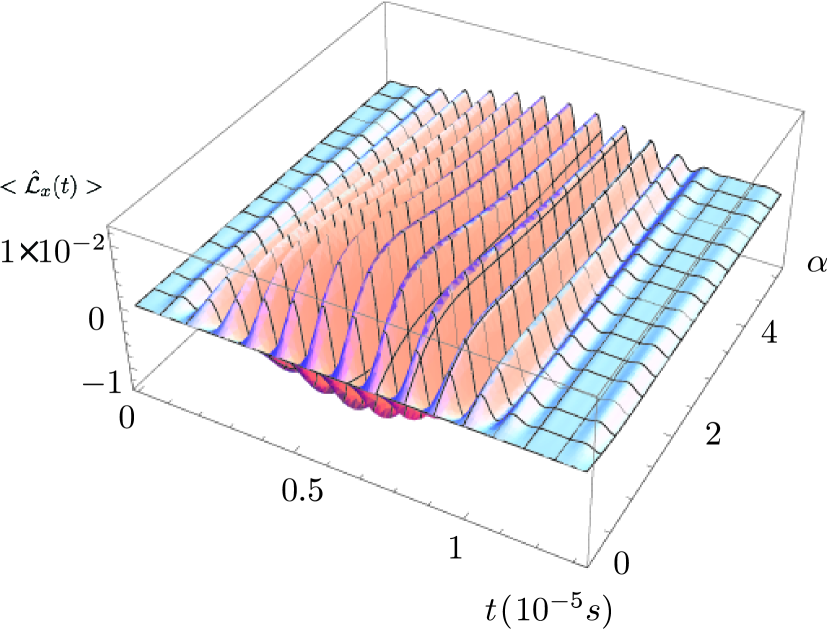
Figure 2: (Color online) Mean value of $\hat{\mathcal{L}}_{x}(t)$ for a cantilever in the initial state as given by Eq. (10) with $C_{0}{=}C_{1}/\alpha{=}1/\sqrt{1+\alpha^{2}}$and $C_{n}=0$ otherwise. The BEC consists of $N{=}10^{3}$ ${}^{87}\text{Rb}$ atoms and $\langle{\hat{\mathcal{L}}_{x,y}(0)}\rangle=0,\;\langle{\hat{\mathcal{L}}_{z}(0)}\rangle=100$. We have used $B_{z}^{0}{=}3\times 10^{-6}\mu T$ and $G_{c}\approx 1.8\times 10^{3}\mu T/\mu$m.

As the qualitative conclusions of our analysis do not depend upon the initial value of the angular momentum component of the spinor, in what follows we shall concentrate on an illustrative example that allows us to clearly display our results. We thus consider, without affecting the generality of our discussions, $\langle\hat{\mathcal{L}}_{x,y}(0)\rangle=0$ and $\langle\hat{\mathcal{L}}_{z}(0)\rangle=100$. When the cantilever and the BEC are uncoupled, we should expect $\langle\hat{\mathcal{L}}_{x}(t)\rangle$ to oscillate at the Larmor frequency $\omega_{L}=g\mu_{B}B_{z}^{0}$ and with an amplitude independent of $\langle\hat{\mathcal{L}}_{x}(0)\rangle$. The BEC-cantilever coupling introduces a modulation of such oscillations and in the following we will demonstrate that the analysis of such oscillatory behavior is indeed useful to extract information on the state of the cantilever.

We first consider the case of a cantilever initially prepared in a superposition of a few eigenstates of the free Hamiltonian $\hat{\mathcal{H}}_{c}^{0}$, as in Eq. (10). In Fig. 2 we show the mean value of $\hat{\mathcal{L}}_{x}(t)$ as a function of the coherence between the states with quantum number $n=0$ and $n=1$, i.e. a state having $C_{0}=C_{1}/\alpha=1/\sqrt{1+\alpha^{2}}$ and $C_{n}=0$ otherwise. One can see a clear modulation of the behavior of $\langle\hat{\cal L}_{x}(t)\rangle$: a close inspection reveals that the carrier frequency $\omega_{L}$ is modulated by the frequency $\omega_{0,1}$. In reality, the Larmor frequency is renormalized as can be seen by the expression for $\Omega_{q}$. However, as we have taken $G_{c}a_{c}\ll B_{z}^{0}$, one can safely assume that the carrier frequency is very close to $\omega_{L}$. Moreover, the maximum of the function is found at $C_{0,1}=1/\sqrt{2}$, which maximizes the coherence between the two states and thus the effect of the modulation. For symmetry reasons, the modulation described is not visible if the cantilever is prepared in a superposition of phonon eigenstates whose quantum numbers are all of the the same parity (such as a single-mode squeezed state). In this case, in fact, the function entering the integral over $q$ in $A_{3}$ is antisymmetric, thus making it vanish. In Fig. 3, $\langle\hat{\mathcal{L}}_{x}(t)\rangle$ is shown for an initial state of the cantilever having $C_{0,1}=C_{2}/\alpha=1/\sqrt{2+\alpha^{2}}$ and $C_{n}=0$ otherwise. It is worth noticing that one can identify two regions of oscillations separated by the line of nodes at $\alpha=1$ where $C_{0}=C_{1}=C_{2}$. We can understand this behavior by studying the amplitudes of oscillation in three $\alpha$-dependent regions. For $\alpha<1$, the main modulation frequency is given by $\omega_{0,1}$ and the role of the third state is to modify the amplitude of the oscillations [see Fig. (3)]. At $\alpha=1$ a destructive interference takes place and the amplitude drops down. For $\alpha>1$ the frequency $\omega_{1,2}$ enters into the evolution of $\langle\hat{\mathcal{L}}_{x}(t)\rangle$ (for parity reasons, the term with frequency $\omega_{0,2}$ has no role) and determines a phase shift of the oscillation fringes. It is interesting to observe that if the initial state of the cantilever is purely thermal, $\langle\hat{\mathcal{L}}_{x}(t)\rangle$ does not oscillate: only quantum coherence in the state of the mechanical system give rise to oscillatory behaviors and their presence is well signaled by the pattern followed by the angular momentum of the spinor-BEC.

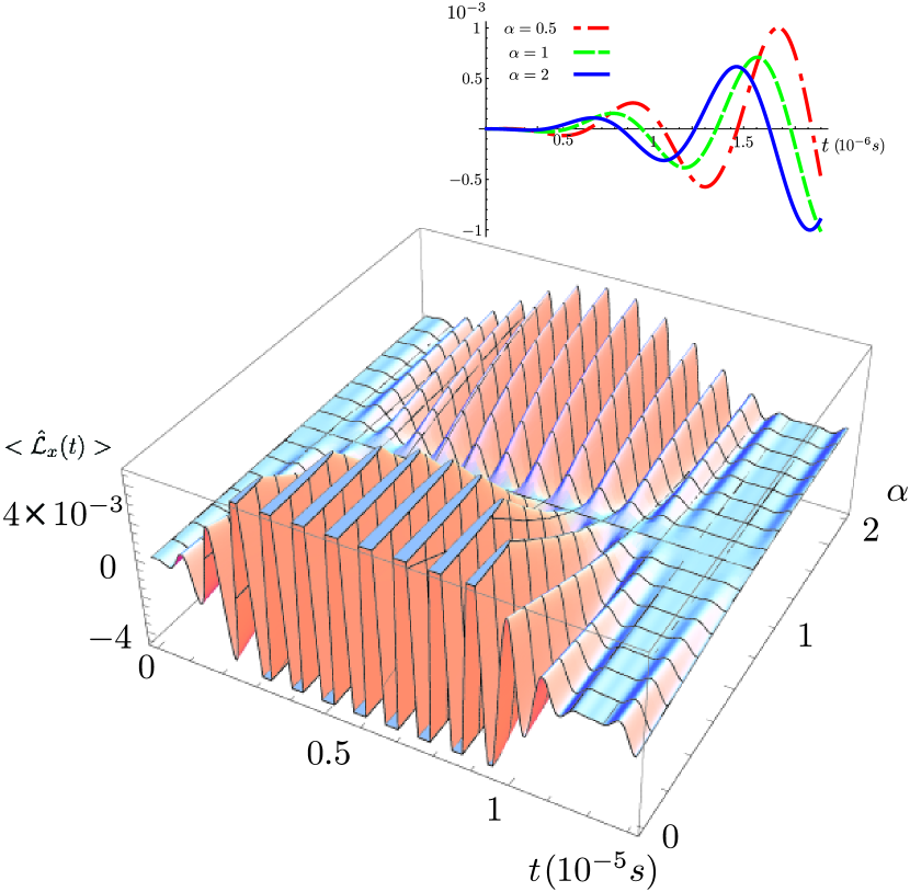
Figure 3: (Color online) Mean value of $\hat{\mathcal{L}}_{x}(t)$ for a cantilever in the initial state as given by Eq. (10) with $C_{0}=C_{1}=C_{2}/\alpha=1/\sqrt{2+\alpha^{2}}$ and $C_{n}=0$ otherwise. The BEC parameters are the same as in Fig. 2. The inset shows that the change in $|\alpha|$ amounts to a shift of the oscillations [we have taken $=e^{i\pi/6}(0.5,1,2)$].

Although the examples considered so far have been instrumental in explaining the connections between the properties of the cantilever and the dynamics of the spinor’s degrees of freedom, they are unfortunately currently far from being realistic. We will therefore now consider closer-to-reality example of a pure state that is likely to be achieved soon. Given the impressive advances in the control and state-engineering of micro and nano-mechanical systems, we will consider the cantilever to be prepared in a coherent state with an average phonon number $n_{ph}$ commentocohe . In Fig. 4 we show the time evolution of $\hat{\mathcal{L}}_{x}(t)$ for $|\alpha|^{2}=1$ [panel (a)], $5$ [panel (b)], $15$ [panel (c)], and $20$ [panel (d)]. One can see that, depending on the mean number of phonons initially present in the mechanical state, new frequencies are introduced in the dynamics of the device: the larger $|\alpha|^{2}$, the larger the number of frequencies involved due to the Poissonian nature of the occupation probability distribution of a coherent state. In Fig. 4 (e), which addresses the case of $|\alpha|^{2}=20$, the study of the dynamics at long evolution times reveals that the carrier frequency is unaffected, for all practical purposes, while the large number of frequencies entering in the evolution gives rise to series of beats occurring at different time scales.

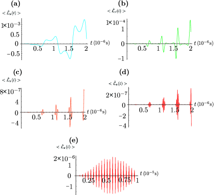
Figure 4: (Color online) Time evolution of $\hat{\mathcal{L}}_{x}$ for a coherent initial state of the cantilever with $|\alpha|^{2}=1\;\;\text{{\bf(a)}},5\;\text{{\bf(b)}},15\;\text{{\bf(c)}},20\;\text{{\bf(d)}}$. For the same parameter as in (d), the plot (e) shows that the carrier frequency $\omega_{L}$ is not significantly affected.

II.2 Detection scheme

To read out the information imprinted on the rotor, one can make use of the Faraday-rotation effect, which allows to measure one component of the the angular momentum of the BEC with only a negligible back action on the condensate itself. It is well-known from classical optics that the linear polarization of an electromagnetic field propagating across an active medium rotates with respect to the direction it had when entering the medium itself. This is the essence of the Faraday-rotation effect, which can be understood by decomposing the initial polarization in terms of two opposite circularly-polarized components experiencing different refractive indices polartensor : by going through the medium, the two components acquire different phases, thus tilting the resulting polarization.

In the case of an ultra-cold gas, an analogous rotation of the polarization of a laser field propagating across the BEC is due to the interaction of light with the atomic spins. If the spins are randomly oriented the net effect is null, while for spins organized in clusters, the effect can indeed be measured. It has been shown in Refs. faradayQNM ; faradayback that the back-action on the BEC induced by this sort of measurements is rather negligible. In recent experiments non destructive measurements on a single BEC of ²³Na atoms have been used to show the dynamical transition between two different regions of the stability diagram of the system faradayNa . This method can thus be effectively used to determine the dynamics of the angular momentum components of the rotor BEC and thus indirectly witness the presence of coherences in the state of the cantilever. Moreover, as shown in Ref. faradayback , the signal to noise ratio (SNR) is proportional to $\sqrt{\tau_{pd}/\tau_{s}}$ where $\tau_{pd}$ is the characteristic time for the response of the photo-detector and $\tau_{s}$ is the average time between consecutive photon-scattering events. In order to be able to detect two distinct events on a time scale $\tau$ we thus need $\tau_{pd}<\tau<\tau_{s}$ to hold. This condition states that the number of scattered photons has to be small enough during the time $\tau$ over which the dynamics we want to resolve occurs. On the other hand the detector “death time” should be smaller than the typical evolution time. While $\tau_{s}$ can be easily tuned by adjusting the experimental working point, ultrafast photo-detectors of the latest generation have response time $\tau_{pd}$ of a few $ps$. As in our scheme we have $\tau\in[10^{-8},10^{-5}]$s, the proposed coherence-probing method appears to be within reach.

III Conclusion

We have considered a mechanical cantilever equipped with a magnetic tip interacting with a spinor Bose-Einstein condensate (BEC) held in an optical trap. The tip produces a magnetic field made up of two components, namely a static one along the tip’s natural anisotropic axes and one perpendicular to it due to the cantilever’s oscillations. By exploiting the mapping of a spinor BEC into a rotor model rotor it is possible to take into account its quantum properties which would have been missed in a mean field theory approach. The BEC is thus mapped onto a quantum gyroscope undergoing a precession about the direction of the magnetic tip’s static field. We have assumed that the cantilever has been cooled down cool ; cool2 to a quantum regime and described it as a quantum harmonic oscillator. We have shown that it is possible to detect the presence of quantumness in the cantilever state in the form of superposition of different eigenstate of the harmonic oscillator. The way to do this is to look at the gyroscopic precession by using Faraday spectroscopy, which in turn only minimally disturbes the BEC dynamics, thus allowing for a continuous probing of the system. Even though we have restricted our analysis to a cantilever equipped with a magnetic molecule it is posible to generalize this scheme to other sorts of mesoscopic magnetic system such as nanotubes.

Note: During completion of this work, a related investigation reporting on the measurement back-action on a vibrating membrane coupled to a BEC has appeared meystre . While the detailed context and general approach differ from ours, this work reinforces the idea that quantum coherence in mechanical systems can be reliably probed by ultracold atomic systems.

- (1) T. J. Kippenberg and K. J. Vahala, Science 321, 1172 (2008); F. Marquardt and S. M. Girvin, Physics 2, 40 (1993); M. Aspelmeyer, S. Gröblacher, K. Hammerer, and N. Kiesel, J. Opt. Soc. Am. B 27, A189 (2010).
- (2) S. Gigan et al., Nature (London) 444, 67 (2006); O. Arcizet et al., ibid.) 444, 71 (2006); A. Schliesser et al., Phys. Rev. Lett. 97, 243905 (2006).
- (3) S. Gröblacher et al., Nature (London) 460, 724 (2009); A. D. O’ Connell et al., ibid. 464, 697 (2010). Donner Nature (London) (2011); Painter Nature (London) (2011).
- (4) M. Paternostro, S. Gigan, M. S. Kim, F. Blaser, H. Böhm, and M. Aspelmeyer, New J. Phys. 8, 107 (2006); M. Paternostro, D. Vitali, S. Gigan, M. S. Kim, C. Brukner, J. Eisert, and M. Aspelmeyer, Phys. Rev. Lett. 99, 250401 (2007).
- (5) P. Treutlein, D. Hunger, S. Camerer, T.W. Hänsch, and J. Reichel, Phys. Rev. Lett. 99, 140403 (2007).
- (6) A.D. Armour and M. Blencowe, New J. Phys. 10, 095004 (2008); J.D. Teufel, T. Donner, Dale Li, J.W. Harlow, M.S. Allman, K. Cicak, A.J. Sirois, J.D. Whittaker, K.W. Lehnert and R.W. Simmonds, Nature (London) 478, 89 (2011); M. Paternostro, G. De Chiara, and G. M. Palma, Phys. Rev. Lett. 104, 243602 (2010); G. De Chiara, M. Paternostro, and G. M. Palma, Phys. Rev. A 83, 052324 (2011); D. Hunger, S. Camerer, M. Korppi, A. Jöckel, T. W. Hänsch, and P. Treutlein, arXiv:1103.1820 (2011).
- (7) D. Hunger, S. Camerer, T. W. Hänsch, D. König, J. P. Kotthaus, J. Reichel, and P. Treutlein, Phys. Rev. Lett. 104, 143002 (2010).
- (8) H. Jing, D. Goldbaum, L. Buchmann, and P. Meystre, Phys. Rev. Lett. 106, 223601 (2011).
- (9) T. L. Ho, Phys. Rev. Lett. 81, 742 (1998); C. K. Law, H. Pu and N. P. Bigelow, ibid. 81, 5257 (1998); T. Ohmi and K. Machida, J. Phys. Soc. Jpn. 67, 1822 (1998).
- (10) Y. Wu, Phys. Rev. A54, 093201 (2001).
- (11) R. Barnett, J. D. Sau, S. Das Sarma Phys. Rev. A82, 031602 (2010); R. Barnett, H.-Y. Hui, C.-H. Lin, J. D. Sau, S. Das Sarma, arXiv:1011.3517 (2010).
- (12) Y. J. Wang, M. Eardley, S. Knappe, J. Moreland, L. Holberg and J. Kitching, Phys. Rev. Lett. 97, 227602 (2006).
- (13) H. Pu, C.K. Law, S. Raghavan, J. H. Eberly and N. P. Bigelow, Phys. Rev. A60, 1463 (1999).
- (14) E.G.M. van Kempen, S.J.J.M.F. Kokkelmans, D.J. Heinzen, B.J. Verhaar, Phys. Rev. Lett. 88, 093201 (2001).
- (15) M.-S Chang, Q Qin, W. Zhang, L.You and M.S. Chapman, Nature Phys. 1, 111 (2005).
- (16) We have inverted the direction of the raising operator as well as the sign of with respect to Ref. spinorham . This does not change the expression for the Hamiltonian in terms of angular momentum operators.
- (17) S. Inouye, M. R. Andrews, J. Stenger, H.J. Miesner, D. M. Stamper-Kurn, W. Ketterle, Nature (London) 392, 151 (1998).
- (18) E. Arimondo, M. Inguscio, P. Violino, Rev. Mod. Phys. 49, 31 (1977).
- (19) The effective mass represents the mass involved in the oscillation of the mode considered, which might be different from the total mass of the cantilever.
- (20) I. H. Deutsch, P. S. Jessen, Phys. Rev. A57, 1972 (1998).
- (21) Y. Takahashi, K. Honda, N. Tanaka, K. Toyoda, K. Ishikawa, T. Yabuzaki Phys. Rev. A60, 4974 (1999).
- (22) G. A. Smith, S. Chaudhury, P. S. Jessen J. Opt. B: Quantum Semiclass. Opt. 5, 323 (2003).
- (23) Y. Liu, E. Gomez, S.E. Maxwell, L.D. Turner, E. Tiesinga, and P.D. Lett, Phys. Rev. Lett. 102, 125301 (2009); ibid. 102, 225301 (2009).
- (24) L. Chang, Q. Zhai, R. Lu, Y. You, Phys. Rev. Lett. 99, 080402 (2007).
- (25) M. Kitagawa, M. Ueda, Phys. Rev. A47, 5138 (1993).
- (26) A mechanical coherent state will be general by displacing, with an intense laser field, the ground state of a cantilever. This is a realistic expectation: current state of the art experiments are only a few quanta away from such an achievement cool2 .
- (27) S. K. Steinke, S. Singh, M. E. Tasgin, P. Meystre, K. C. Schwab, and M. Vengalattore, Phys. Rev. A84, 023841 (2011).