Efficient emulators of computer experiments using compactly supported correlation functions, with an application to cosmology

Abstract

Statistical emulators of computer simulators have proven to be useful in a variety of applications. The widely adopted model for emulator building, using a Gaussian process model with strictly positive correlation function, is computationally intractable when the number of simulator evaluations is large. We propose a new model that uses a combination of low-order regression terms and compactly supported correlation functions to recreate the desired predictive behavior of the emulator at a fraction of the computational cost. Following the usual approach of taking the correlation to be a product of correlations in each input dimension, we show how to impose restrictions on the ranges of the correlations, giving sparsity, while also allowing the ranges to trade off against one another, thereby giving good predictive performance. We illustrate the method using data from a computer simulator of photometric redshift with 20,000 simulator evaluations and 80,000 predictions.

, , ,
and

t1Supported in part by NSF Grant DMS-06-35449 to the Statistical and Applied Mathematical Sciences Institute.

t2Supported in part by a grant from the Natural Sciences and Engineering Research Council of Canada.

t3Supported in part by the Department of Energy under contract W-7405-ENG-36.

Simulation of complex systems has become commonplace in scientific studies. Frequently, simulators (or computer models) are computationally demanding, and relatively few evaluations can be performed. In other cases, the computer models are fast to evaluate but are not readily available to all scientists. This arises, for example, when the simulator runs only on a supercomputer or must be run by specialists. In either case, a statistical emulator of the computer model can act as a surrogate, providing predictions of the computer model output at unsampled inputs values, with corresponding measures of uncertainty [see, e.g., Sacks et al. (1989), Santner, Williams and Notz (2003)]. The emulator can serve as a component in probabilistic model calibration [Kennedy and O’Hagan (2001)], and it can help provide insight into the functional form of the simulator response and the importance of various inputs [Oakley and O’Hagan (2004)].

Building an emulator can be viewed as a type of nonparametric regression problem, but with a key difference. Computer experiments differ from their real-world counterparts in that they are typically deterministic. That is, running the code twice with the same set of input values will produce the same result. To deal with this difference from the usual noisy settings, Sacks et al. (1989) proposed modeling the response from a computer experiment as a realization from a Gaussian process (GP). From a Bayesian viewpoint, one can think of the GP as a prior distribution over the class of functions produced by the simulator.

The GP model is particularly attractive for emulation because of its flexibility to fit a large class of response surfaces. It is also desirable that the statistical model, and corresponding prediction intervals, reflect some type of smoothness assumption regarding the response surface, leading to zero (or very small) predictive uncertainty at the design points, small predictive uncertainty close to the design points, and larger uncertainty further away from the design points. For example, note the behavior of the confidence intervals in the illustration shown in panel (a) of Figure 1.

(a)	(b)
(c)	(d)

Figure 1: Illustrative example in which the data were drawn from a mean zero Gaussian process with covariance function $K(x,x^{\prime})=\exp\{-5|x-x^{\prime}|^{1.5}\}$ and predictions were made using one of four methods. Each plot shows the observations (solid dots), predictions (solid line) and pointwise 95% confidence intervals for the predictions (gray bands). The models were (a) zero mean GP with the correct covariance structure, (b) OLS using Legendre polynomials up to degree 6, (c) zero mean GP with the Bohman correlation function (7), with $\tau=0.1$, and (d) GP with Legendre polynomials up to degree 2 in the mean and Bohman correlation function with $\tau=0.1$.

The main drawback of the usual GP model in our setting is that it can be computationally infeasible for large designs. The likelihood for the observations is multivariate normal, and evaluation of this density for $n$ design points requires manipulations of the $n\times n$ covariance matrix that grow as $O(n^{3})$. This limitation is the main motivation for this article, which was prompted by our work on just such an application in cosmology (see Section 5). Here, the basic idea is to construct a statistical model based on a set of simulated data consisting of multi-color photometry for training set galaxies, as well as the corresponding true redshifts. Given photometric information for a test galaxy, the system should produce an estimated value for the true redshift. The very large experimental design used to explore the input space, that is, the large number of galaxies used to build the training set, presents a computational challenge for the GP.

It is worth noting that the GP model is not the only approach for emulating computer simulators. Using a GP with constant mean term can be viewed as a way of forcing the covariance structure of the GP to model all the variability in the computer output. At the other extreme, one can take a regression based approach and treat the errors as white noise, as in An and Owen (2001). This approach has the benefit of being computationally efficient, as the correlation matrix is now the identity matrix. However, it does not have the attractive property of a smooth GP, namely, that the predictive distribution interpolates the observed data and that the uncertainty reflects the above properties. Instead, the white noise is introducing random error to the problem that is not actually believed to exist; it is there simply to reflect lack of fit. The implications of this for predictive uncertainty are illustrated in panels (a) and (b) of Figure 1. Panel (a) shows a set of data fit using the standard GP model, and panel (b) shows the same data fit using ordinary least squares regression with the set of Legendre polynomials up to degree six. The behavior in panel (a) is what we desire in an emulator, but the model is computationally intractable for large data sets. The model in panel (b) is very efficient from a computational standpoint, but the predictions do not reflect the determinism of the computer simulator. The approach proposed in this article can be viewed as finding an intermediate model to those in panels (a) and (b), such that the model is both fast to fit and has the appropriate behavior for prediction.

In this article, we propose new methodology for emulating computer simulators when $n$ is large (i.e., when it is infeasible to fit the usual GP model). The approach makes the key innovation of replacing the covariance function with one that has compact support. This has the effect of introducing zeroes into the covariance matrix, so that it can be efficiently manipulated using sparse matrix algorithms. In addition, the proposed approach easily handles the anisotropy that is common in computer experiments by allowing the correlation range in each dimension to vary and also imposes a constraint on these ranges to enforce a minimum level of sparsity in the covariance matrix. We further propose a model for the mean of the GP, rather than taking it to be a scalar. The motivation for this is that the introduction of regression functions tends to decrease the estimated correlation length in the GP, thereby offsetting some of the loss of predictive efficiency introduced by using a compactly supported covariance. Last, we propose prior distributions to incorporate experimenter belief and also to make the application of regression terms and the compactly supported covariance function efficiently work together.

In the next section we introduce the GP that is commonly used for building emulators and illustrate the challenges for large data sets. In Section 3 we present new methodology for building computationally efficient emulators, and we give some details of the implementation and computational advantages in Section 4. In Section 5 we investigate the performance of the method in a simulation study. The method is then used to construct an emulator of photometric redshifts of cosmological objects in Section 6, and we conclude with some final remarks in the Appendix.

1 Gaussian process models for computer experiments

Consider a simulator that takes inputs $\mathbf{x}\in\Re^{d}$ and produces univariate output $Y(\mathbf{x})$. The GP model generally used in this setting treats the response as a realization of a random function:

$$Y({\mathbf{x}})=\sum_{i=1}^{p}f_{i}({\mathbf{x}})\beta_{i}+Z({\mathbf{x}}),$$ (1)

where $f_{1},\ldots,f_{p}$ are fixed regression functions, ${\bolds\beta}=(\beta_{1},\ldots,\beta_{p})^{\prime}$ is a vector of unknown regression coefficients, and $Z$ is a mean zero GP. The covariance function of $Z$ is denoted by

$$\operatorname{Cov}(Z({\mathbf{x}}),Z({\mathbf{x}}^{\prime}))=K({\mathbf{x}},{\mathbf{x}}^{\prime};\sigma^{2},\bolds\theta)=\sigma^{2}R({\mathbf{x}},{\mathbf{x}}^{\prime};\bolds\theta),$$ (2)

where $\sigma^{2}$ is the marginal variance of $Z$ and $\bolds\theta$ is a vector of parameters controlling the correlation.

We defer until the end of this section a discussion of the choice of $f_{1},\ldots,f_{p}$ and $R$ and first lay out some general notation. Let $\mathbf{Y}=(Y(\mathbf{x}_{1}),\ldots,Y(\mathbf{x}_{n}))^{\prime}$ be the vector of observed responses. Then, ignoring a constant, the log-likelihood under this model is $l({\bolds\beta},\bolds\theta,\sigma^{2})=-{\frac{1}{2}\log}|\mathbf{R}(\bolds\theta)|-\frac{1}{2\sigma^{2}}(\mathbf{Y}-\break\mathbf{F}{\bolds\beta})^{\prime}\mathbf{R}(\bolds\theta)^{-1}(\mathbf{Y}-\mathbf{F}{\bolds\beta})$, where $\mathbf{F}$ is the $n\times p$ matrix of regression functions and $\mathbf{R}(\bolds\theta)$ is the $n\times n$ matrix of correlations with $[\mathbf{R}(\bolds\theta)]_{ij}=R(\mathbf{x}_{i},\mathbf{x}_{j};\bolds\theta)$. In addition, for any set of model parameters, the conditional distribution of $Y(\mathbf{x}_{0})$ at a new input value, $\mathbf{x}_{0}$, given the observations $\mathbf{Y}$, is normal with mean and variance

$$E[Y(\mathbf{x}_{0})|\mathbf{Y},\bolds\beta,\sigma^{2},\bolds\theta] = f(\mathbf{x}_{0}){\bolds\beta}+\mathbf{r}_{0}(\bolds\theta)^{\prime}\mathbf{R}(\bolds\theta)^{-1}(\mathbf{Y}-\mathbf{F}{\bolds\beta}),$$ (3)

$$\operatorname{Var}[Y(\mathbf{x}_{0})|\mathbf{Y},\bolds\beta,\sigma^{2},\bolds\theta] = \sigma^{2}[1-\mathbf{r}_{0}(\bolds\theta)^{\prime}\mathbf{R}(\bolds\theta)^{-1}\mathbf{r}_{0}(\bolds\theta)],$$ (4)

where $\mathbf{r}_{0}(\bolds\theta)$ is the $n$-vector of correlations between the observed responses and $Y(\mathbf{x}_{0})$.

In practice, $\bolds\beta$, $\sigma^{2}$ and $\bolds\theta$ are unknown and must be estimated. This can be achieved using likelihood-based methods such as maximum likelihood (ML) or restricted maximum likelihood (REML) [see, e.g., Irvine, Gitelman and Hoeting (2007) for a comparison of ML and REML estimation]. Alternatively, one may specify a Bayesian model in which the joint posterior distribution for both parameters and predicted values of the function can be approximated via Markov Chain Monte Carlo (MCMC). We adopt the latter approach, although most of the proposed methodology is also applicable in a frequentist setting.

Two choices must be made to complete the specification in (1) and (2), the regression functions $f_{1},\ldots,f_{p}$ and the correlation function $R$. The mean structure in (1) is almost always taken to be flat over the domain of the function, with $f(x)\equiv 1$. By far the most common specification for the correlation function is a product of one-dimensional power exponential correlation functions. Specifically, writing $\bolds\theta_{k}=\{\phi_{k},\alpha_{k}\}$,

$$R({\mathbf{x}},{\mathbf{x}}^{\prime};\bolds\theta) = \prod_{k=1}^{d}R_{k}(|x_{k}-x_{k}^{\prime}|;{\bolds\theta}_{k})\qquad\mbox{(Product form)}$$ (5)

$$= \prod_{k=1}^{d}\exp\{-\phi_{k}|x_{k}-x_{k}^{\prime}|^{\alpha_{k}}\}\qquad\mbox{(Power exponential)}$$ (6)

for $\phi_{k}>0$ and $1\leq\alpha_{k}\leq 2$. Since the ${\bolds\phi}_{k}$’s are not constrained to be equal, the model can handle different signals in each input dimension of the simulator (i.e., anisotropy). This choice of constant mean term and power exponential correlation is so common in practice that we will refer to it as the “standard model.” In the next section we shall diverge from the standard model and propose a more computationally efficient model with different mean and covariance structures.

No matter what choices are made for the regression terms and correlation function, inference and prediction for this model requires evaluation of the log-likelihood, typically many times. These calculations require finding the log determinant of $\mathbf{R}(\bolds\theta)$ and solving $\mathbf{R}(\bolds\theta)^{-1}(\mathbf{Y}-\mathbf{F}{\bolds\beta})$. When the correlation functions are strictly positive, as in the standard model, both of these grow in complexity by order $n^{3}$, and therein lies the problem. These operations are intractable for moderate sample sizes and simply impossible for large sample sizes. It is this problem that motivates the current work.

2 Building computationally efficient emulators

Our approach is conceptually straightforward, consisting of three main innovations: [(2)]

using compactly supported correlation functions to model small-scale variability,

using regression functions in the mean of the GP to model large-scale variability, and

specifying prior distributions for model parameters (or parameter constraints, in the frequentist case) that are flexible while still enforcing computational efficiency. These three innovations work together to produce a flexible, fast and powerful method for computer model emulation.

2.1 Compactly supported correlation functions

We begin by proposing that the correlation functions in the product covariance (5) are chosen to have compact support. That is, for some $\tau_{k}\geq 0$, $R_{k}(|x_{k}-x_{k}^{\prime}|;\tau_{k})=0$ when $|x_{k}-x_{k}^{\prime}|\geq\tau_{k}$. This has the effect of introducing zeros into the covariance matrix, so computationally efficient sparse matrix techniques [Pissanetzky (1984), Barry and Pace (1997)] may be used. Compactly supported correlation functions have recently received increased attention in the literature, used either by themselves [Gneiting (2002), Stein (2008)] or multiplying another, strictly positive correlation function, which is known as tapering [Furrer, Genton and Nychka (2006), Kaufman, Schervish and Nychka (2008)]. These applications all assume that the compactly supported correlation function is isotropic, requiring a single range parameter. In contrast, anisotropic covariance functions are the norm for computer experiments because the inputs to the computer model are frequently on different scales and/or impact the response in vastly different ways. Therefore, we use correlation functions with compact support in product form.

We focus on two families of models that can be used to approximate the power exponential function (6). These functions are zero for $t\geq\tau$, and for $t<\tau$,

$$\mbox{Bohman:}\hskip 22.0pt\quad R(t;\tau) = (1-t/\tau)\cos(\pi t/\tau)+\sin(\pi t/\tau)/\pi,$$ (7)

$$\qquad\mbox{Truncated power:}\quad R(t;\tau,\alpha,\nu) = [1-(t/\tau)^{\alpha}]^{\nu},$$ (9)

$$\eqntext{0<\alpha<2,\nu\geq\nu_{d}(\alpha).}$$

The term $\nu_{d}(\alpha)$ in (9) represents a restriction so that the function is a valid correlation, with $\lim_{\alpha\rightarrow 2}\nu_{d}(\alpha)=\infty$ [Golubov (1981)]. Although it is difficult to calculate $\nu_{d}(\alpha)$ exactly, Gneiting (2001) gives upper bounds for a variety of values of $\alpha$ between 1.5 and 1.955. For example, upper bounds for $\nu_{1}(\alpha)$ when $\alpha=3/2$ and $5/3$ are 2 and 3, respectively.

These two functions allow for some flexibility in the smoothness of the realizations of the GP, in loose analogy to the parameter $\alpha$ in the power exponential model (6). The truncated power function (9) is not differentiable even once at the origin, with $\alpha<2$, corresponding to a process which is not even mean square continuous, as for (6) with $\alpha<2$. In contrast, the Bohman function (7) is twice differentiable at the origin, corresponding to a process which is mean square differentiable. Of course, when $\alpha=2$, the power exponential function (6) is infinitely differentiable at the origin. However, we feel this level of smoothness is often unrealistic, and in our applied work we have not found any reason to prefer a higher level of smoothness than is given by (7).

Note that the ranges play two different roles in our approach. First, they control the degree of correlation in each dimension. In this way they are similar to the range parameters $\phi_{k}$ in the power exponential function (6). However, unlike the $\phi_{k}$, the $\tau_{k}$ also control the degree of sparsity of the correlation matrix. To produce computational savings, some restrictions must be applied to the $\tau_{k}$. We chose to do this through the prior distribution, which we discuss in Section 2.3.

2.2 Regression functions

We propose using regression functions to model the mean structure of a computer model, rather than the constant mean used in the standard model. The intuition behind our approach is that if the large-scale structure of the simulator output is well captured by a linear combination of the basis functions $f_{i}$, we would naturally expect the residual process $Z({\mathbf{x}})$ to have shorter-range correlations. This type of trade-off between large scale and small scale variability has been noted in the spatial statistics literature [Cressie (1993), Stein (2008)], and it was noted in the results of a simulation study of computer experiments by Welch et al. (1992). However, to our knowledge, it has not previously been exploited for computational purposes in constructing emulators, an application in which we will see the often high dimensionality of the input ${\mathbf{x}}$ allows this trade-off to be leveraged particularly well.

Using a richer mean structure produces more efficient predictions than the use of the compactly supported covariance alone. For example, panel (c) of Figure 1 illustrates the predictions and pointwise confidence bands under the zero mean GP model with Bohman correlation function (7) with $\tau=0.1$. These are obviously less efficient than the results under the true correlation function in panel (a). However, this limitation can be addressed by incorporating regression terms. Panel (d) in Figure 1 illustrates the results of combining a small set of basis functions with a compactly supported correlation function. The behavior of the predictions is similar to that in panel (a), but the model in panel (d) can be applied to large data sets, whereas the model in (a) cannot.

There are a variety of basis functions among which one can choose, and detailing them is not the focus of this article. We have found a good default choice to be taking $f_{i}$ to be tensor products of Legendre polynomials over $[0,1]$, the input variable in each dimension having been rescaled to this domain [see, e.g., An and Owen (2001)].

2.3 Prior distributions

The full specification of our Bayesian model requires that we choose prior distributions for the parameters $\bolds\tau$, $\sigma^{2}$ and $\bolds\beta$. We advocate the inclusion of prior information where available, but describe here a default choice of prior distributions that brings additional computational efficiency. These advantages may be had in a frequentist setting by replacing the prior distributions with certain restrictions on the parameter space, which should be obvious as we proceed.

One of the novel features of the proposed approach is use of an anisotropic compactly supported covariance and the estimation of the range parameters. Recall that the $\tau_{k}$’s play the role of governing the correlation in each dimension and also controlling the computational complexity of the model. Unfortunately, the mapping from a collection $\tau_{1},\ldots,\tau_{d}$ to the sparsity of a given matrix will depend on the particular configuration of sampling points, and it is also difficult to translate a degree of sparsity (measured, say, by the percentage of off-diagonal zeroes) to computation time for a particular algorithm. However, we have found that with a bit of trial and error, controlling the sparsity of the correlation matrix $\mathbf{R}$ can be an adequate proxy for controlling computation time. The question then is, how do we control sparsity through the prior for ${\bolds\tau}$?

Throughout, we will assume that all input variables have been scaled to $[0,1]$, so that taking $\tau_{k}>1$ for all $k$ introduces no sparsity. A simple restriction is

$$\tau_{j}\leq B\qquad\mbox{for all }j,B>0.$$ (10)

However, using this restriction in creating a prior distribution ignores an important advantage of using compactly supported correlation functions within the product correlation given in (5): that $R(x,x^{\prime})\geq 0$ only if $|x_{j}-x^{\prime}_{j}|<\tau_{j}$ for all $j=1,\ldots,d$. That is, a pair of observations having zero correlation in any dimension will be independent and contribute a zero to the overall correlation matrix. Therefore, the $\tau_{j}$ may trade off against one another to produce the same degree of sparsity. Therefore, we restrict $\tau$ further by taking $\tau$ to be uniformly distributed over the space

$$T_{C}=\Biggl{\{}\tau\in\Re^{d}\dvtx\tau_{j}\geq 0\mbox{ }\forall d,\sum_{j=1}^{d}\tau_{j}\leq C\Biggr{\}},\qquad C>0.$$ (11)

This can be thought of as defining the prior distribution over a $d$-dimensional triangle rather than a cube. Because of the trade-off between the $\tau_{j}$ discussed above, $C$ can generally be greater than $B$ is in (10) and impose the same degree of sparsity. That is, some of the $\tau_{j}$ are allowed to be large, which they may indeed need to be to reflect a high degree of correlation in particular input dimensions. Some trial and error may be required to find a $C$ for which calculations can actually be carried out; we return to this in the next section. This restriction may not work well for the case that certain input variables have no impact on the output variable over the range being simulated, which would correspond to $\tau_{j}\rightarrow\infty$. We make the assumption that such variables have been previously identified and fixed during a prior screening analysis such as described in Welch et al. (1992) or Linkletter et al. (2006).

Finally, we specify prior distributions for $\sigma^{2}$ and $\bolds\beta$. We follow Berger, De Oliveira and Sansó (2001) and Paulo (2005), who proposed the form $p(\sigma^{2},\beta,\tau)\propto\pi(\tau)/\sigma^{2}$ for Gaussian processes. As our choice of $\pi$ is a proper density, it can be shown that this choice still produces a proper posterior [Berger, De Oliveira and Sansó (2001)]. One advantage of this choice is that $\beta$ and $\sigma^{2}$ may be easily integrated out of the model, so that posterior sampling may be done only over the vector $\tau$.

We end this section with a note relating our proposed model to existing works in the field of spatial statistics, in which estimation and prediction under large sample sizes has seen much recent development. These approaches may be characterized broadly as either approximating the likelihood for the original model, or changing the model itself to one that is computationally more convenient. Examples of the former include Stein, Chi and Welty (2004) and Kaufman, Schervish and Nychka (2008), while a common modification to the model itself is to represent the random field in terms of a lower-dimensional random variable; models falling under this framework are reviewed by Wikle (2010). The approach we take in this paper is to change the model rather than approximate it. We did consider using compactly supported correlation functions as an approximation tool rather than using them directly, following Kaufman, Schervish and Nychka (2008). Ultimately, however, since there is no “true” random process generating the output of the computer simulator, we decided to take the conceptually simpler approach of modifying the model itself. That is, in this nonparametric regression context, the GP is simply a tool for expressing prior beliefs about the function, and this may be done effectively using compactly supported correlation functions when regression terms are also included in the model.

3 Implementation and computational considerations

Implementation of these methods for a given data set proceeds in two steps. The first step is to sample from the posterior distribution $p(\bolds\tau|\mathbf{Y})$ using a Metropolis sampler. As noted above, our choice of prior distribution allows us to work with this marginal distribution, integrating out $\sigma^{2}$ and $\bolds\beta$. This leads to additional computational savings, as we can sample the vector $\bolds\tau$ using an efficient, adaptive Metropolis sampler, the details of which are described in the Appendix. The second step is to use these samples to generate predictions at new input values. Rather than incorporating this into the sampler, we recommend another computational trick here, which is to calculate conditional means and variances at a subset of the iterations (i.e., conditional on $\bolds\tau^{(i)}$) and use these to reconstruct the predictive mean and variance using laws of iterated expectation. The details of this calculation are also described in the Appendix. In the remainder of this section, we outline the computational savings to be gained from our approach, compared to standard, nonsparse techniques.

The demanding aspects of the calculations all involve $\mathbf{R}(\bolds\tau)$, the correlation matrix for a particular value of $\bolds\tau$. To efficiently calculate the quantities involved, after we propose a new $\bolds\tau$ in the Metropolis step, we first compute a sparse representation of $\mathbf{R}(\bolds\tau)$, then compute the quantities which will be used in calculating the integrated likelihood. Here, we use the spam package in R [Furrer and Sain (2010)], which uses the efficient “old Yale sparse format” for representing sparse matrices, where only the nonzero elements, column indices and row pointers are stored. From a computational viewpoint, operations involving the zero elements need not be performed. The time-consuming steps in evaluating the likelihood are then as follows: [(2)]

Identifying pairs of input values ${\mathbf{x}}_{i}$ and ${\mathbf{x}}_{j}$ such that $|x_{ik}-x_{jk}|<\tau_{k}$, $\forall k=1,\ldots,d$. (All other pairs will contribute a zero to the matrix.)

For only these pairs, computing $\prod_{k=1}^{d}R_{k}(|x_{ik}-x_{jk}|;\tau_{k})$ and using only these to create the sparse representation of $\mathbf{R}(\bolds\tau)$.

Computing the Cholesky decomposition of the sparse matrix object, that is, $\mathbf{Q}(\bolds\tau)$ such that $\mathbf{R}(\bolds\tau)=\mathbf{Q}(\bolds\tau)^{\prime}\mathbf{Q}(\bolds\tau)$.

Backsolving to compute $(\mathbf{Q}(\bolds\tau)^{\prime})^{-1}\mathbf{Y}$ and $(\mathbf{Q}(\bolds\tau)^{\prime})^{-1}\mathbf{F}$.

Figure 2 shows the average number of seconds required to carry out these steps for a reference data set consisting of locations uniformly sampled over the input space $[0,1]^{4}$, which

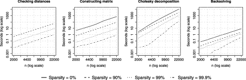
Figure 2: Number of seconds required to carry out each step in evaluating the likelihood, for varying degrees of sparsity and sample sizes. The case “$\mbox{Sparsity}=0$%,” shown as a solid line, corresponds to using a strictly positive correlation function, while for the other cases “Sparsity” denotes the percentage of off-diagonal elements in the matrix that are equal to zero. The “Checking distances” step only applies to the algorithm used for compactly supported correlation functions, which is why no solid line appears in this plot. All measurements are shown on the log (base 10) scale, and each gridline along the y-axis corresponds to one order of magnitude.

is the same dimension as our example in Section 5. The calculations were carried out for various sample sizes and varying degrees of sparsity, which is imposed by the choice of the cutoff $C$. Each calculation was repeated 10 times, and the number of seconds required for each were averaged to produce the plot. Computations were performed on a Dell quad socket machine with four dual-core AMD Opteron 2.4 GHz CPUs and 8 GB of RAM. All axes are on the log scale. In particular, each gridline along the y-axis corresponds to one order of magnitude. Overall, we can see that using a sparse correlation function reduces most of the calculations by one to three orders of magnitude.

4 Simulation study

The method we present here is intended for use in situations in which the “standard” method is computationally infeasible. However, it is instructive to see how our method compares when $n$ is small enough that the standard method can actually be implemented. In this section we compare the performance of our proposed model to that of the standard model, when the data are actually simulated under the standard model. Of course, in practice, neither model is “correct,” since the object of interest is a deterministic function, not a realization of a stochastic process, but this framework allows us to compare the efficiency of predictions made under varying degrees of smoothness and for different correlation lengths.

In carrying out the simulation study, we vary both the distribution of the data and the choices made in fitting it. Regarding the data, we consider processes in two or four dimensions, with correlation function (6) with $\alpha_{k}$ set equal (in all dimensions) to 1.5 or 1.99. (We do not consider the infinitely smooth case of $\alpha=2$ here, to avoid dealing on a case-by-case basis with the numerical instabilities that sometimes arise.) We specify $\phi_{k}$ in (6) to be such that the effective range, defined as the distance beyond with correlations are less than 0.05, is either 0.5 or 2 in all dimensions. This gives six possible combinations.

For each combination and each of 100 replications of the simulation, we consider sample sizes of $n=100,150,250,400,650$ and $1\mbox{,}100$. The design (choice of input settings) for each $n$ and replication is generated using a random Latin hypercube sample (LHS) [McKay, Beckman and Conover (1979)] on $[0,1]^{d}$. In addition, we generate a set of $n_{\mathrm{pred}}=512$ input settings at which to predict the function, using the orthogonal array-based Latin hypercube sampling (OA-LHS) algorithm by Tang (1993), with frequency $\lambda=2$. We sampled values of $Y(x)$ over the LHS and OA-LHS jointly, corresponding to a realization from the GP. The rationale for this sampling strategy stems from our different priorities when choosing the design points and choosing the prediction points. Repeated sampling under simple LHS is our attempt to mimic the broad class of designs experimenters mights use in practice. To best evaluate the predictive accuracy of our methods over that class, however, we use OA-LHS to choose the evaluation points, due to its superiority over simple LHS in integral approximation.

In fitting each data set and making the predictions, we either use the standard model with the $\alpha_{k}$ set to the value used in simulating the data, or we use the method outlined in the previous section. For the latter, we have some choices to make. The first is the basis functions $f_{i}$ to include in (1). We use fifth order Legendre polynomials in each dimension. Specifically, we include all main effects up to order five, as well as all interactions involving two dimensions, in which the sum of the maximum power of the exponent in each dimension is constrained to be less than or equal to $5$. For example, in two dimensions, this implies using terms involving $x_{1},\ldots,x_{1}^{5},x_{2},\ldots,x_{2}^{5},x_{1}x_{2},x_{1}x_{2}^{2},\ldots,x_{1}^{4}x_{2}$. We have investigated the impact of the order of the polynomial for the regression functions and have found that fourth or fifth order polynomials are sufficient for most applications. We do not try here to adapt the order of the polynomial to each particular data set. In practice, we recommend routinely using a subset of the data and performing ordinary least squares regression for increasing degrees of the polynomial. The smallest degree of the polynomial where the fit is satisfactory is chosen to be the order used in the approach (more on this in Section 5.1).

The final choice is the value of the cutoff $C$ in (11). Here we chose $C$ such that the maximum proportion of off-diagonal elements was either 0.02 or 0.05, both of which reflect a high degree of sparsity, as we would often be required to specify in practice. The truncated power correlation function (9) is used; the Bohman function (7) gives very similar results.

The predictions are compared using two criteria. The first, sometimes called the Nash–Sutcliffe efficiency, is equal to

$$\mathrm{NSE}=1-\frac{\sum_{x\in\mathcal{X}_{\mathrm{pred}}}(\hat{Y}(x)-Y(x))^{2}}{\sum_{x\in\mathcal{X}_{\mathrm{pred}}}(Y(x)-\bar{Y})^{2}}.$$ (12)

Here, $\hat{Y}(x)$ represents the mean of the posterior predictive distribution for $Y(x)$ given the vector of observations $\mathbf{Y}$, while $\bar{Y}$ represents the mean of $\mathbf{Y}$. Predictions are made at the set of 500 hold out points, $\mathcal{X}_{\mathrm{pred}}$. The second term of (12) is the ratio of an estimate of the predictive mean square error to the unstandardized variance of $Y(x)$. Thus, the NSE has an interpretation similar to $R^{2}$ in linear regression, insofar as it represents an estimate of the proportion of the variability in $\mathbf{Y}$ that is explained by the model, although measured on an out-of-sample test set. We estimate the average value of (12) across repeated samples by calculating it for each iteration of the simulation study and then averaging over iterations. We do not expect NSE to be better (larger) for our method compared to the standard method, since we know we are using a different model to fit than to generate the data. However, comparing this under various conditions can help us build intuition about when the proposed method will perform well. The second criterion we consider is the empirical coverage probability of the 95% prediction intervals, measured both across the range of the input space and across repeated samples.

We begin by comparing the NSE of the sparse method to that of the standard method. Figure 3 plots NSE under the eight different combinations of dimension, power $\alpha$, and effective

Figure 3: Nash–Sutcliffe efficiencies for predictions made using the posterior mean. In each panel, the solid lines corresponds to the data-generating model, while the dashed and dotted lines correspond to the proposed method with a maximum proportion of off-diagonal elements of 0.02 or 0.05, respectively.

range for which the data were generated. First examine the NSE for the standard method, shown by the solid lines in each panel. It is clear that the prediction task ranges quite a bit in difficulty across the range of eight conditions, from processes that are difficult to predict given the data (e.g., small NSE) to those which allow very high accuracy predictions (with NSE close to 1). The prediction problem is harder in four dimensions than in two, simply due to a lower data density. Also, not surprisingly, the smoother and flatter the process realizations, the easier they are to predict. That is, holding other variables constant, the standard method has higher NSE when the power is 1.99 rather than 1.5, and when the effective range is 2.0 rather than 0.5.

Now examine the NSE for the sparse method. Not surprisingly, within each panel the NSE is larger when the proportion of nonzero off-diagonal elements is allowed to be 5% (dotted line) rather than only 2% (dashed line). However, these differences are minor compared to the differences across the different processes. Another interesting trend that emerges is that, compared to the standard method, the sparse method tends to perform quite well as the sample size gets large. In most cases, by $n=1\mbox{,}100$ the sparse method is still capturing about the same amount of the total variability as the standard method. The proposed method does perform relatively worse when the process is hard to predict, but even in these cases a large proportion of the variability is explained. In light of the fact that we have not expended any effort in determining the degree of the polynomial for each realization of the GP, the results are even more encouraging. For the large sample sizes for which the method was designed, we expect the NSE to be close to 1.

Next, consider the empirical coverage probabilities of the 95% prediction intervals. Figure 4 shows the observed

Figure 4: Empirical coverage probabilities for pointwise credible intervals. In each panel, the solid line corresponds to the data-generating model, while the dashed and dotted lines correspond to the proposed method with a maximum proportion of off-diagonal elements of 0.02 or 0.05, respectively.

coverage rates, under the same setup as in Figure 3. Not surprisingly, under the data-generating model, the coverage rates are close to the nominal rate of 95%. (The rates would be theoretically exact if we were not also estimating the range parameters.) Under the proposed model, the rates are often more conservative than the nominal rate, particularly when the input has only two dimensions. Although the widths of the intervals decrease with $n$, they do not decrease rapidly enough to maintain only 95% coverage, a fact that is attributable to the shorter correlation ranges being imposed for the sake of sparsity. This is a potential drawback to using the proposed model, although we remind the reader that the results under the data-generating model are not possible for large $n$; this is what motivates the approximation. These results should also not be taken to be representative of all simulators one might encounter in practice. In the application in Section 5, for example, exploratory analysis with a held-out sample suggests the coverage under the proposed model is very close to the nominal rate. In that example, posterior samples for the range parameters are well away from the boundary imposed for sparsity.

5 Application to photometric redshifts

A major aim of upcoming cosmological surveys is to characterize the nature of dark energy, a mysterious type of energy that is driving a current epoch of acceleration in the expansion of the Universe [for a recent review, see Frieman, Turner and Huterer (2008)]. Evidence for cosmic acceleration first came from measurements of the optical luminosity from a specific class of supernovae [Riess et al. (1998), Perlmutter et al. (1999)]. In a matter-dominated Universe, the expansion rate should slow down with time, and the aim was to verify that the Universe was expanding more rapidly in the past by studying distant supernovae. Instead, observations indicated the Universe was doing exactly the opposite. So puzzling is this behavior that understanding dark energy—a hypothesized form of mass-energy accounting for the acceleration, or perhaps signaling the breakdown of general relativity on very large lengthscales—is considered to be one of the major unsolved problems in all of physical science.

Information about dark energy can be inferred in a variety of ways, some of which depend on an accurate three-dimensional representation of galaxies in a cosmological survey. It is straightforward to determine the angular location of an object in the sky, but the fundamental difficulty is determining the distance with sufficient accuracy. In large scale structure studies, the analogue of radial distance is the cosmological redshift. Due to cosmic expansion, the wavelength of light received from a distant object is stretched (“redshifted”), with more distant objects being at greater redshifts. Accurate redshift determination requires measurement of the spectrum of each galaxy at high resolution, but this is very difficult and too time-consuming for the very large numbers of very distant, hence very dim, galaxies. An alternative is to obtain galaxy photometry (flux measurements) in a restricted number of wavebands, and to attempt to reconstruct the redshift from just this information. Redshifts obtained in this way are termed “photometric” redshifts, in contrast to the more accurate “spectroscopic” redshifts. To obtain a photometric redshift estimate, however, requires estimating the functional relationship between the observations within the wavebands and the spectroscopic redshift.

The simulation we consider here models this relationship for four different wavebands. It simulates the true spectroscopic redshift and corresponding photometric measurements for the Dark Energy Survey [Abbott et al. (2005), Oyaizu et al. (2006)], which will come online in the near future. The training and validation data sets were generated to be of size 20,000 and 80,000, respectively. The design points were not chosen systematically, but were rather sampled from distributions meant to mimic what will be encountered in data from the Dark Energy Survey. The analysis in this article treats the simulation as the usual noiseless computer model case, with inputs corresponding to the flux measurements in the four wavebands and output corresponding to the spectroscopic redshift. There is some expected intrinsic scatter due to coarsening of information, potential degeneracies, and the fact that the predictors can be viewed as often having error themselves. Nonetheless, we expect that the GP will be able to efficiently predict the spectroscopic redshift from model inputs.

Our analysis proceeds in two steps. We first carry out an exploratory analysis on a small subset of the training data, so that we may explore the effects of various modeling choices before implementing these choices on the entire data set. Interestingly, we show here that the methods outlined in this paper in fact outperform the standard model in both predictive as well as computational efficiency. That is, the computationally efficient methods that allow us to scale up and work with the full data set do not come at a cost to predictive efficiency; they actually have higher Nash–Sutcliffe efficiency than the traditional, computationally infeasible methods. This gives us confidence in proceeding to the second step of the analysis, which is to fit the model on the set of 20,000 training points and evaluate the predictions at the 80,000 validation points.

5.1 Preliminary analysis and model comparison

We first normalize the input space so that each input variable lies within $[0,1]$. We sample a smaller “training” and “validation” set from the full training set of 20,000; these have size 2,000 and 500, respectively, which is small enough to fit the standard model for comparison.

The first question to be addressed in this exploratory analysis is the choice of basis functions $f_{i}$ in (1). As in the simulation study, we consider various tensor products of Legendre polynomials over $[0,1]$. Let $p$ represent the maximum degree, that is, the maximum power in a main effect for a single input dimension, or the maximum sum of powers in an interaction. Let $m$ represent the maximum number of dimensions that may be involved in an interaction. Then a simple way to evaluate the choice of $p$ and $m$ is to find the ordinary least squares estimates $\hat{\beta}$ for each choice using the $n=2\mbox{,}000$ training set and evaluate the Nash–Sutcliffe efficiency of predictions $X_{0}\hat{\beta}$ for $X_{0}$ consisting of the corresponding regression terms evaluated at the validation input set with $n=500$. This is shown in Figure 5. The choice $p=4$ and $m=2$ produces the largest NSE, of 0.799, and produces relatively few regression terms ($q=53$) compared to the sample size: here 2,000, later 20,000. Although matrix multiplication requires many fewer evaluations than the solution of a linear system of equivalent size, it can still be problematic if both $q$ and $n$ are large, so it is a happy coincidence that the choice of $p$ and $m$ that has highest NSE for this data is also computationally efficient.

Figure 5: Nash–Sutcliffe efficiency (NSE) of predictions made using OLS estimates and various choices of maximum degree $p$ and maximum interacting dimensions $m$ (indicated by number on the plot). The choice $p=4$ and $m=2$ produces the highest NSE and includes relatively few regression terms ($q=53$) compared to the sample size.

We now fit the model (1) with all combinations of the following choices:

• the covariance structure $R$ in (2) set to either the power exponential function (6) or a product of truncated power functions (9) in each dimension,

• the parameter $\alpha$ in (6) and (9) set either to 1, $3/2$ or $5/3$ in each dimension,

• the mean including an intercept only ($q=1$) or a regression on tensor products of Legendre polynomials as described above, with $p=4$ and $m=2$.

In all models, we used the prior specification $p(\sigma^{2},\beta)\propto 1/\sigma^{2}$. We took the prior for $\bolds\phi$ in (6) to be uniform over a hyper-cube, and, as specified in (11), we took the prior for $\tau$ to be uniform over a hyper-triangle. In particular, we took the cutoff $C=0.185$, chosen so that the proportion of off-diagonal elements in the correlation matrix that were nonzero would be at most 2%. This imposes a very high degree of sparsity, and in this initial exploratory analysis we can determine the effect of this choice on the posterior distribution for $\bolds\tau$.

For each of the twelve modeling combinations, we sampled from the posterior distribution for model parameters and used this to generate predictions and pointwise credible intervals for the validation set. Table 1 shows the Nash–Sutcliffe efficiency for each modeling combination, and Table 2 shows the empirical coverage probabilities. First note that the largest NSE in Table 1 is for the sparse correlation structure (9) with power $\alpha=1$ and Legendre polynomials up to degree 4, followed closely by the same model with $\alpha=3/2$. This relationship holds across all entries in rows three and four of the table, corresponding to a model with $q=53$ regression terms. It is interesting to note that this trend reverses in the first two rows, corresponding to the intercept only model. This provides evidence that in our method, both components—compactly supported correlation structure as well as a more structured mean term—are needed to achieve good predictive accuracy. Table 2 shows that the empirical coverage of the prediction intervals is very close to the nominal 95% level when using regression terms and a sparse correlation. This again gives us confidence in our method.

=300pt $\bolds{\mathrm{Power}=1}$ $\bolds{\mathrm{Power}=3/2}$ $\bolds{\mathrm{Power}=5/3}$ $\mathrm{Degree}=0$ Nonsparse 0.791 0.773 0.757 Sparse 0.702 0.659 0.617 $\mathrm{Degree}=4$ Nonsparse 0.839 0.818 0.761 Sparse 0.849 0.848 0.843

Table 1: Nash–Sutcliffe efficiencies for predictions made using the posterior mean

=300pt $\bolds{\mathrm{Power}=1}$ $\bolds{\mathrm{Power}=3/2}$ $\bolds{\mathrm{Power}=5/3}$ $\mathrm{Degree}=0$ Nonsparse 0.936 0.928 0.908 Sparse 0.960 0.950 0.948 $\mathrm{Degree}=4$ Nonsparse 0.952 0.926 0.906 Sparse 0.954 0.952 0.952

Table 2: Empirical coverage probabilities for posterior predictive intervals

There is one final comparison we make using this preliminary test set. This is for the sparse methods only, corresponding to rows two and four of the tables. Note that the prior distribution restricts $\sum_{j=1}^{4}\tau_{j}\leq C$, where we chose $C=0.185$. Figure 6 shows the trace plots of this sum over iterations of the Metropolis sampler, discarding an initial

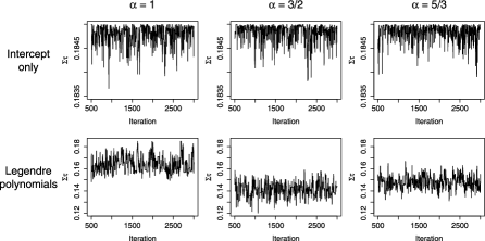
Figure 6: Trace plots for $\sum_{j=1}^{4}\tau_{j}$ over iterations in the Metropolis sampler. Introducing regression terms into the mean of the Gaussian process (degree${}={}$4) produces much better mixing, as well as the potential for increased computational efficiency.

burn-in period. Note another major implication of using the Legendre polynomials: it changes the posterior distribution for $\bolds\tau$, so that the posterior distribution of the sum moves away from this boundary. In contrast, in the intercept only model, the posterior samples of $\bolds\tau$ are varying only slightly around the upper boundary of 0.185. (Note the difference in scales between rows in Figure 6.) Another way of saying this is that a cutoff of $C=0.185$ is too small for the intercept only GP model to capture all the variability in the data set, but it is adequate to capture variability in the residuals after introducing the Legendre polynomials. This has implications both for mixing of the sampler, which is much better in the models with the regression terms, and for computational efficiency, as we see that the cutoff $C$ can be reduced even further, as far as 0.16 when the power $\alpha=3/2$. The smaller this cutoff, the larger the computational savings, as it allows us to rule out more pairs of input values before the MCMC even begins to run. For this reason, as well as observing that the Nash–Sutcliffe efficiency when $\alpha=3/2$ was only very slightly larger than the optimal one in Table 1, we choose to use this setting when working with the full data set.

5.2 Full analysis

In the second stage of the analysis, we fit the model using the full set of $20\mbox{,}000$ training points and made predictions at each of the $80\mbox{,}000$ validation points. We sampled $B=3\mbox{,}000$ MCMC iterations using the Gibbs sampling algorithm described in Section 3 and the Appendix, discarding the first 500 for burn-in. For every tenth iteration thereafter, we calculated the conditional means and variances of the predictive distribution for $Y(x_{0})$ given the observations and the parameter values at that iteration, from which we formed Monte Carlo approximations of the mean and variance of the posterior predictive distribution, as also described in the Appendix. The posterior means for the 80,000 new input values are shown in Figure 7, plotted against the actual spectroscopic redshift

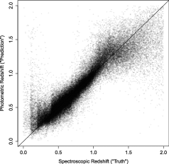
Figure 7: Photometric redshift predictions and the corresponding spectroscopic redshift values from the simulator. Points are plotted with transparency, so that dark areas of the plot indicate a high density of points being over-plotted in the same region.

values. The Nash–Sutcliffe efficiency for the predictions is 0.831, and the empirical coverage rate for the 95% credible intervals is close to the nominal level, at 94%.

6 Discussion

In this article we have proposed new methodology for analyzing large computer experiments using a GP. The approach uses an anisotropic compactly supported covariance, as well as a regression function for mean, to emulate the computer model. With respect to the latter adaptation, we have proposed the use of a flat prior distribution for the regression parameters $\bolds\beta$, using a preliminary study to select the set of basis functions to be used. This provides additional computational efficiency, as all parameters except $\bolds\tau$ may be integrated out of the model. Given the model selection problem, which we solve in a rather ad-hoc way, one might also be tempted to incorporate a model selection or model averaging approach. For example, one approach we examined was to err on the side of including more basis functions, but to use a shrinkage prior for $\bolds\beta$, with

$$\beta_{i}|\xi_{i} \stackrel{{\scriptstyle\mathrm{indep}}}{{\sim}} N(0,\xi_{i}),\qquad i=1,\ldots,p,$$

$$\xi_{i} \stackrel{{\scriptstyle\mathrm{i.i.d.}}}{{\sim}} IG(a,b),\qquad i=1,\ldots,p.$$

The prior specification in (6) is akin to a generalized ridge regression, in which each coefficient receives its own shrinkage weight $w_{i}=\xi_{i}/(1+\xi_{i})$ [Denison and George (2000)]. Despite the elegance of this approach, we found that it contributed very little to the predictive efficiency of our method; it increased the Nash–Sutcliffe efficiency by only a few percentage points, and then only for small data sets, not the type that motivate our work. In our judgement, the added computational cost is not worth this small potential improvement. Instead, we advocate the simpler and computationally more efficient approach of choosing the basis functions based on a random subset of the data in a preliminary study, as described in Section 5.

We also note that the inclusion of the regression terms in the mean of the GP has implications for extrapolation beyond the range of the initial input values. Although polynomial regression can be problematic when it comes to extrapolation, it is unclear that the behavior obtained under a constant mean term is more desirable. In the standard model, when one is far from the initial input values, the GP prediction returns to the global mean and does not depend on the new inputs at all. Indeed, Bayarri et al. (2007) suggest using a more complicated mean structure to avoid this problem. The fact that neither approach is entirely satisfactory reflects the difficulty of extrapolation, and users should be aware of the implications of the structure of the mean term if it must be undertaken.

Appendix: Posterior sampling and prediction

To generate samples from the posterior distribution $p(\bolds\tau|\mathbf{Y})$, we use an adaptive Metropolis algorithm, taking the transition density to be a multivariate normal random walk. At iteration $i$, we sample a candidate $\bolds\tau^{\mathrm{cand}}|\allowbreak\bolds\tau^{(i-1)}\sim\mathit{MVN}(\bolds\tau^{(i-1)},\Sigma^{(i)})$, where $\Sigma^{(i)}$ is calculated adaptively using an algorithm to be described shortly. If the candidate value falls outside of the constrained parameter space $T_{C}$, as defined in (11), it is immediately rejected and we set $\bolds\tau^{(i)}=\bolds\tau^{(i-1)}$. Otherwise, we calculate the integrated likelihood $L^{I}(\bolds\tau^{\mathrm{cand}})$, where

$$L^{I}({\bolds\tau})\propto|\bolds\Gamma({\bolds\tau})|^{-1/2}|\mathbf{F}^{\prime}\bolds\Gamma({\bolds\tau})^{-1}\mathbf{F}|^{-1/2}(\hat{\sigma}^{2}({\bolds\tau}))^{(n-p)/2}$$

for $\hat{\sigma}^{2}({\bolds\tau})=(\mathbf{Y}-\mathbf{F}{\hat{\beta}}({\bolds\tau}))^{\prime}\bolds\Gamma({\bolds\tau})^{-1}(\mathbf{Y}-\mathbf{F}\hat{\beta}({\bolds\tau}))$ and $\hat{\beta}({\bolds\tau})=(\mathbf{F}^{\prime}\bolds\Gamma({\bolds\tau})^{-1}\mathbf{F})^{-1}\mathbf{F}^{\prime}\times\bolds\Gamma({\bolds\tau})^{-1}\mathbf{Y}$. The computationally demanding aspects of this calculation are described in Section 3. We then set $\bolds\tau^{(i)}=\bolds\tau^{\mathrm{cand}}$ with probability$\max\{L^{I}(\bolds\tau^{\mathrm{cand}})/L^{I}(\bolds\tau^{(i-1)}),1\}$ and $\bolds\tau^{(i-1)}$ otherwise.

We adapt the proposal covariance matrix using the Log-Adaptive Proposal algorithm of Shaby and Wells (2011), a slightly modified version of Algorithm 4 in Andrieu and Thoms (2008). The algorithm periodically updates an estimate of the posterior covariance matrix and then takes the proposal covariance matrix to be a scaled version of this, the scaling factor also being updated. This allows the sampler to target a particular acceptance rate and thereby increase efficiency. Although using previous states to generate the proposal violates the Markov property of the chain, the ergodicity of the process is maintained within a framework of “vanishing adaptation” [Roberts and Rosenthal (2009)].

After sampling from the posterior distribution for $\bolds\tau$, the second step is to generate samples from the posterior predictive distribution for the output of the simulator at new input values. Let $\mathbf{Y}_{0}$ denote this new output. One could generate a sample from $p(\mathbf{Y}_{0}|\mathbf{Y},\bolds\tau)$ at each iteration of the MCMC. However, since we are primarily interested in the mean and variance of the predictive distribution, we instead adopt the computationally more stable approach of calculating conditional means and variances at each iteration (i.e., conditional on $\bolds\tau^{(i)}$) and using these to reconstruct the predictive mean and variance. Specifically, for a subset of the $\bolds\tau$ samples (the number of which may be chosen based on an estimate of the smallest effective sample size among the elements of $\bolds\tau$), we calculate the mean and variance of $\mathbf{Y}_{0}$ given $\mathbf{Y}$ and $\bolds\tau^{(i)}$, to produce $\mathbf{m}^{(i)}$ and $\mathbf{v}^{(i)}$. As

$$\pmatrix{\mathbf{Y}\cr\mathbf{Y}_{0}}\big{|}\sigma^{2},\bolds\beta,\bolds\tau\sim\mathit{MVN}\left(\pmatrix{\mathbf{X}\cr\mathbf{X}_{0}}\bolds\beta,\sigma^{2}\pmatrix{\bolds\Gamma(\bolds\tau)&\bolds\gamma(\bolds\tau)\cr\bolds\gamma^{\prime}(\bolds\tau)&\bolds\Gamma_{0}(\bolds\tau)}\right),$$

$p(\mathbf{Y}_{0}|\mathbf{Y},\bolds\tau^{(i)})$ is multivariate t, with $\mathbf{m}^{(i)}\,{=}\,\hat{Y}_{0}(\bolds\tau^{(i)})$ and $\mathbf{v}^{(i)}\,{=}\,\frac{n-q}{n-q-2}\hat{\sigma}^{2}(\bolds\tau^{(i)})\times\mathbf{V}(\bolds\tau^{(i)})$, for

$$\hat{\mathbf{Y}}_{0}(\bolds\tau) = \mathbf{X}_{0}\hat{\beta}(\bolds\tau)+\bolds\gamma^{\prime}(\bolds\tau)\bolds\Gamma(\bolds\tau)^{-1}[\mathbf{Y}-\mathbf{X}\hat{\beta}(\bolds\tau)],$$

$$\hat{\beta}(\bolds\tau) = \bigl{(}\mathbf{X}^{\prime}\bolds\Gamma(\bolds\tau)^{-1}\mathbf{X}\bigr{)}^{-1}\mathbf{X}^{\prime}\bolds\Gamma(\bolds\tau)^{-1}\mathbf{Y},$$

$$\hat{\sigma}^{2}(\bolds\tau) = \bigl{(}\mathbf{Y}-\mathbf{X}\hat{\beta}(\bolds\tau)\bigr{)}^{\prime}\bolds\Gamma(\bolds\tau)^{-1}\bigl{(}\mathbf{Y}-\mathbf{X}\hat{\beta}(\bolds\tau)\bigr{)}/\mathbf{n},$$

$$V(\bolds\tau) = \bolds\Gamma_{0}(\bolds\tau)-\bolds\gamma(\bolds\tau)^{\prime}\bolds\Gamma(\bolds\tau)^{-1}\bolds\gamma(\bolds\tau)+\mathbf{X}_{0}\bigl{(}\mathbf{X}^{\prime}\bolds\Gamma(\bolds\tau)^{-1}\mathbf{X}\bigr{)}^{-1}\mathbf{X}_{0}.$$

Finally, we use Monte Carlo approximation to estimate $E[\mathbf{Y}(\mathbf{x}_{0})|\mathbf{Y}]$ and $\operatorname{Var}[\mathbf{Y}(\mathbf{x}_{0})|\mathbf{Y}]$ from the $K$ samples according to

$$E[\mathbf{Y}(\mathbf{x}_{0})|\mathbf{Y}] = E[E[\mathbf{Y}(\mathbf{x}_{0})|\mathbf{Y},\bolds\tau]]$$

$$\approx \frac{1}{K}\sum_{i=1}^{K}\mathbf{m}^{(i)}\equiv\bar{\mathbf{m}},$$

$$\operatorname{Var}[\mathbf{Y}(\mathbf{x}_{0})|\mathbf{Y}] = E[\operatorname{Var}[\mathbf{Y}(\mathbf{x}_{0})|\mathbf{Y},\bolds\tau]]+\operatorname{Var}[E[\mathbf{Y}(\mathbf{x}_{0})|\mathbf{Y},\bolds\tau]]$$

$$\approx \frac{1}{K}\sum_{i=1}^{K}\mathbf{v}^{(i)}+\frac{1}{K}\sum_{i=1}^{K}\bigl{(}\mathbf{m}^{(i)}-\bar{\mathbf{m}}\bigr{)}^{2}.$$

These can be used to construct approximate pointwise credible intervals for $Y(\mathbf{x}_{0})$ given $\mathbf{Y}$. If global intervals are needed, one should instead sample from the corresponding multivariate $t$ conditional distributions at each iteration.

References

- Abbott et al. (2005) {bmisc}[author] \bauthor\bsnmAbbott, \bfnmT\binitsT. \betalet al. (\byear2005). \bhowpublishedThe dark energy survey. Preprint. Available at Astro-ph/ 0510346. \bptokimsref \endbibitem
- An and Owen (2001) {barticle}[mr] \bauthor\bsnmAn, \bfnmJian\binitsJ. and \bauthor\bsnmOwen, \bfnmArt\binitsA. (\byear2001). \btitleQuasi-regression. \bjournalJ. Complexity \bvolume17 \bpages588–607. \biddoi=10.1006/jcom.2001.0588, issn=0885-064X, mr=1881660 \bptokimsref \endbibitem
- Andrieu and Thoms (2008) {barticle}[mr] \bauthor\bsnmAndrieu, \bfnmChristophe\binitsC. and \bauthor\bsnmThoms, \bfnmJohannes\binitsJ. (\byear2008). \btitleA tutorial on adaptive MCMC. \bjournalStat. Comput. \bvolume18 \bpages343–373. \biddoi=10.1007/s11222-008-9110-y, issn=0960-3174, mr=2461882 \bptokimsref \endbibitem
- Barry and Pace (1997) {barticle}[author] \bauthor\bsnmBarry, \bfnmR. P.\binitsR. P. and \bauthor\bsnmPace, \bfnmR. K.\binitsR. K. (\byear1997). \btitleKriging with large data sets using sparse matrix techniques. \bjournalComm. Statist. Simulation Comput. \bvolume26 \bpages619–629. \bptokimsref \endbibitem
- Bayarri et al. (2007) {barticle}[mr] \bauthor\bsnmBayarri, \bfnmMaria J.\binitsM. J., \bauthor\bsnmBerger, \bfnmJames O.\binitsJ. O., \bauthor\bsnmPaulo, \bfnmRui\binitsR., \bauthor\bsnmSacks, \bfnmJerry\binitsJ., \bauthor\bsnmCafeo, \bfnmJohn A.\binitsJ. A., \bauthor\bsnmCavendish, \bfnmJames\binitsJ., \bauthor\bsnmLin, \bfnmChin-Hsu\binitsC.-H. and \bauthor\bsnmTu, \bfnmJian\binitsJ. (\byear2007). \btitleA framework for validation of computer models. \bjournalTechnometrics \bvolume49 \bpages138–154. \biddoi=10.1198/004017007000000092, issn=0040-1706, mr=2380530 \bptokimsref \endbibitem
- Berger, De Oliveira and Sansó (2001) {barticle}[mr] \bauthor\bsnmBerger, \bfnmJames O.\binitsJ. O., \bauthor\bsnmDe Oliveira, \bfnmVictor\binitsV. and \bauthor\bsnmSansó, \bfnmBruno\binitsB. (\byear2001). \btitleObjective Bayesian analysis of spatially correlated data. \bjournalJ. Amer. Statist. Assoc. \bvolume96 \bpages1361–1374. \biddoi=10.1198/016214501753382282, issn=0162-1459, mr=1946582 \bptokimsref \endbibitem
- Cressie (1993) {bbook}[mr] \bauthor\bsnmCressie, \bfnmNoel A. C.\binitsN. A. C. (\byear1993). \btitleStatistics for Spatial Data. \bpublisherWiley, \baddressNew York. \bidmr=1239641 \bptokimsref \endbibitem
- Denison and George (2000) {bmisc}[author] \bauthor\bsnmDenison, \bfnmD.\binitsD. and \bauthor\bsnmGeorge, \bfnmE.\binitsE. (\byear2000). \bhowpublishedBayesian prediction using adaptive ridge estimators. Technical report, Dept. Mathematics, Imperial College, London, UK. \bptokimsref \endbibitem
- Frieman, Turner and Huterer (2008) {barticle}[author] \bauthor\bsnmFrieman, \bfnmJ. A.\binitsJ. A., \bauthor\bsnmTurner, \bfnmM. S.\binitsM. S. and \bauthor\bsnmHuterer, \bfnmD.\binitsD. (\byear2008). \btitleDark energy and the accelerating universe. \bjournalAnnual Review of Astronomy and Astrophysics \bvolume46 \bpages385–432. \bptokimsref \endbibitem
- Furrer, Genton and Nychka (2006) {barticle}[mr] \bauthor\bsnmFurrer, \bfnmReinhard\binitsR., \bauthor\bsnmGenton, \bfnmMarc G.\binitsM. G. and \bauthor\bsnmNychka, \bfnmDouglas\binitsD. (\byear2006). \btitleCovariance tapering for interpolation of large spatial datasets. \bjournalJ. Comput. Graph. Statist. \bvolume15 \bpages502–523. \biddoi=10.1198/106186006X132178, issn=1061-8600, mr=2291261 \bptokimsref \endbibitem
- Furrer and Sain (2010) {barticle}[author] \bauthor\bsnmFurrer, \bfnmReinhard\binitsR. and \bauthor\bsnmSain, \bfnmStephan R.\binitsS. R. (\byear2010). \btitlespam: A sparse matrix R package with emphasis on MCMC methods for Gaussian Markov random fields. \bjournalJournal of Statistical Software \bvolume36 \bpages1–25. \bptokimsref \endbibitem
- Gneiting (2001) {barticle}[mr] \bauthor\bsnmGneiting, \bfnmTilmann\binitsT. (\byear2001). \btitleCriteria of Pólya type for radial positive definite functions. \bjournalProc. Amer. Math. Soc. \bvolume129 \bpages2309–2318 (electronic). \biddoi=10.1090/S0002-9939-01-05839-7, issn=0002-9939, mr=1823914 \bptokimsref \endbibitem
- Gneiting (2002) {barticle}[mr] \bauthor\bsnmGneiting, \bfnmTilmann\binitsT. (\byear2002). \btitleCompactly supported correlation functions. \bjournalJ. Multivariate Anal. \bvolume83 \bpages493–508. \biddoi=10.1006/jmva.2001.2056, issn=0047-259X, mr=1945966 \bptokimsref \endbibitem
- Golubov (1981) {barticle}[mr] \bauthor\bsnmGolubov, \bfnmB. I.\binitsB. I. (\byear1981). \btitleOn Abel–Poisson type and Riesz means. \bjournalAnal. Math. \bvolume7 \bpages161–184. \biddoi=10.1007/BF01908520, issn=0133-3852, mr=0635483 \bptokimsref \endbibitem
- Irvine, Gitelman and Hoeting (2007) {barticle}[mr] \bauthor\bsnmIrvine, \bfnmKathryn M.\binitsK. M., \bauthor\bsnmGitelman, \bfnmAlix I.\binitsA. I. and \bauthor\bsnmHoeting, \bfnmJennifer A.\binitsJ. A. (\byear2007). \btitleSpatial designs and properties of spatial correlation: Effects on covariance estimation. \bjournalJ. Agric. Biol. Environ. Stat. \bvolume12 \bpages450–469. \biddoi=10.1198/108571107X249799, issn=1085-7117, mr=2405534 \bptokimsref \endbibitem
- Kaufman, Schervish and Nychka (2008) {barticle}[mr] \bauthor\bsnmKaufman, \bfnmCari G.\binitsC. G., \bauthor\bsnmSchervish, \bfnmMark J.\binitsM. J. and \bauthor\bsnmNychka, \bfnmDouglas W.\binitsD. W. (\byear2008). \btitleCovariance tapering for likelihood-based estimation in large spatial data sets. \bjournalJ. Amer. Statist. Assoc. \bvolume103 \bpages1545–1555. \biddoi=10.1198/016214508000000959, issn=0162-1459, mr=2504203 \bptokimsref \endbibitem
- Kennedy and O’Hagan (2001) {barticle}[mr] \bauthor\bsnmKennedy, \bfnmMarc C.\binitsM. C. and \bauthor\bsnmO’Hagan, \bfnmAnthony\binitsA. (\byear2001). \btitleBayesian calibration of computer models. \bjournalJ. R. Stat. Soc. Ser. B Stat. Methodol. \bvolume63 \bpages425–464. \biddoi=10.1111/1467-9868.00294, issn=1369-7412, mr=1858398 \bptokimsref \endbibitem
- Linkletter et al. (2006) {barticle}[mr] \bauthor\bsnmLinkletter, \bfnmCrystal\binitsC., \bauthor\bsnmBingham, \bfnmDerek\binitsD., \bauthor\bsnmHengartner, \bfnmNicholas\binitsN., \bauthor\bsnmHigdon, \bfnmDavid\binitsD. and \bauthor\bsnmYe, \bfnmKenny Q.\binitsK. Q. (\byear2006). \btitleVariable selection for Gaussian process models in computer experiments. \bjournalTechnometrics \bvolume48 \bpages478–490. \biddoi=10.1198/004017006000000228, issn=0040-1706, mr=2328617 \bptokimsref \endbibitem
- McKay, Beckman and Conover (1979) {barticle}[mr] \bauthor\bsnmMcKay, \bfnmM. D.\binitsM. D., \bauthor\bsnmBeckman, \bfnmR. J.\binitsR. J. and \bauthor\bsnmConover, \bfnmW. J.\binitsW. J. (\byear1979). \btitleA comparison of three methods for selecting values of input variables in the analysis of output from a computer code. \bjournalTechnometrics \bvolume21 \bpages239–245. \bidissn=0040-1706, mr=0533252 \bptokimsref \endbibitem
- Oakley and O’Hagan (2004) {barticle}[mr] \bauthor\bsnmOakley, \bfnmJeremy E.\binitsJ. E. and \bauthor\bsnmO’Hagan, \bfnmAnthony\binitsA. (\byear2004). \btitleProbabilistic sensitivity analysis of complex models: A Bayesian approach. \bjournalJ. R. Stat. Soc. Ser. B Stat. Methodol. \bvolume66 \bpages751–769. \biddoi=10.1111/j.1467-9868.2004.05304.x, issn=1369-7412, mr=2088780 \bptokimsref \endbibitem
- Oyaizu et al. (2006) {binproceedings}[author] \bauthor\bsnmOyaizu, \bfnmH.\binitsH., \bauthor\bsnmCunha, \bfnmC.\binitsC., \bauthor\bsnmLima, \bfnmM.\binitsM., \bauthor\bsnmLin, \bfnmH.\binitsH. and \bauthor\bsnmFrieman, \bfnmJ.\binitsJ. (\byear2006). \btitlePhotometric redshifts for the Dark Energy Survey. In \bbooktitleBulletin of the American Astronomical Society \bvolume38 \bpages140. \bptokimsref \endbibitem
- Paulo (2005) {barticle}[mr] \bauthor\bsnmPaulo, \bfnmRui\binitsR. (\byear2005). \btitleDefault priors for Gaussian processes. \bjournalAnn. Statist. \bvolume33 \bpages556–582. \biddoi=10.1214/009053604000001264, issn=0090-5364, mr=2163152 \bptokimsref \endbibitem
- Perlmutter et al. (1999) {barticle}[author] \bauthor\bsnmPerlmutter, \bfnmS.\binitsS., \bauthor\bsnmAldering, \bfnmG.\binitsG., \bauthor\bsnmGoldhaber, \bfnmG.\binitsG., \bauthor\bsnmKnop, \bfnmRA\binitsR., \bauthor\bsnmNugent, \bfnmP.\binitsP., \bauthor\bsnmCastro, \bfnmPG\binitsP., \bauthor\bsnmDeustua, \bfnmS.\binitsS., \bauthor\bsnmFabbro, \bfnmS.\binitsS., \bauthor\bsnmGoobar, \bfnmA.\binitsA., \bauthor\bsnmGroom, \bfnmDE\binitsD. \betalet al. (\byear1999). \btitleMeasurements of [Omega] and [Lambda] from 42 high-redshift supernovae. \bjournalThe Astrophysical Journal \bvolume517 \bpages565–586. \bptokimsref \endbibitem
- Pissanetzky (1984) {bbook}[mr] \bauthor\bsnmPissanetzky, \bfnmSergio\binitsS. (\byear1984). \btitleSparse Matrix Technology. \bpublisherAcademic Press, \baddressLondon. \bidmr=0751237 \bptokimsref \endbibitem
- Riess et al. (1998) {barticle}[author] \bauthor\bsnmRiess, \bfnmA. G.\binitsA. G., \bauthor\bsnmFilippenko, \bfnmA. V.\binitsA. V., \bauthor\bsnmChallis, \bfnmP.\binitsP., \bauthor\bsnmClocchiatti, \bfnmA.\binitsA., \bauthor\bsnmDiercks, \bfnmA.\binitsA., \bauthor\bsnmGarnavich, \bfnmP. M.\binitsP. M., \bauthor\bsnmGilliland, \bfnmR. L.\binitsR. L., \bauthor\bsnmHogan, \bfnmC. J.\binitsC. J., \bauthor\bsnmJha, \bfnmS.\binitsS., \bauthor\bsnmKirshner, \bfnmR. P.\binitsR. P. \betalet al. (\byear1998). \btitleObservational evidence from supernovae for an accelerating universe and a cosmological constant. \bjournalAstronomical Journal \bvolume116 \bpages1009–1038. \bptokimsref \endbibitem
- Roberts and Rosenthal (2009) {barticle}[mr] \bauthor\bsnmRoberts, \bfnmGareth O.\binitsG. O. and \bauthor\bsnmRosenthal, \bfnmJeffrey S.\binitsJ. S. (\byear2009). \btitleExamples of adaptive MCMC. \bjournalJ. Comput. Graph. Statist. \bvolume18 \bpages349–367. \biddoi=10.1198/jcgs.2009.06134, issn=1061-8600, mr=2749836 \bptnotecheck year\bptokimsref \endbibitem
- Sacks et al. (1989) {barticle}[mr] \bauthor\bsnmSacks, \bfnmJerome\binitsJ., \bauthor\bsnmWelch, \bfnmWilliam J.\binitsW. J., \bauthor\bsnmMitchell, \bfnmToby J.\binitsT. J. and \bauthor\bsnmWynn, \bfnmHenry P.\binitsH. P. (\byear1989). \btitleDesign and analysis of computer experiments. \bjournalStatist. Sci. \bvolume4 \bpages409–435. \bidissn=0883-4237, mr=1041765 \bptnotecheck related\bptokimsref \endbibitem
- Santner, Williams and Notz (2003) {bbook}[mr] \bauthor\bsnmSantner, \bfnmThomas J.\binitsT. J., \bauthor\bsnmWilliams, \bfnmBrian J.\binitsB. J. and \bauthor\bsnmNotz, \bfnmWilliam I.\binitsW. I. (\byear2003). \btitleThe Design and Analysis of Computer Experiments. \bpublisherSpringer, \baddressNew York. \bidmr=2160708 \bptokimsref \endbibitem
- Shaby and Wells (2011) {bmisc}[author] \bauthor\bsnmShaby, \bfnmB.\binitsB. and \bauthor\bsnmWells, \bfnmM. T.\binitsM. T. (\byear2011). \bhowpublishedExploring an adaptive Metropolis algorithm. Technical Report 2011-14, Dept. Statistical Science, Duke Univ., Durham, NC. \bptokimsref \endbibitem
- Stein (2008) {barticle}[mr] \bauthor\bsnmStein, \bfnmMichael L.\binitsM. L. (\byear2008). \btitleA modeling approach for large spatial datasets. \bjournalJ. Korean Statist. Soc. \bvolume37 \bpages3–10. \biddoi=10.1016/j.jkss.2007.09.001, issn=1226-3192, mr=2420389 \bptokimsref \endbibitem
- Stein, Chi and Welty (2004) {barticle}[mr] \bauthor\bsnmStein, \bfnmMichael L.\binitsM. L., \bauthor\bsnmChi, \bfnmZhiyi\binitsZ. and \bauthor\bsnmWelty, \bfnmLeah J.\binitsL. J. (\byear2004). \btitleApproximating likelihoods for large spatial data sets. \bjournalJ. R. Stat. Soc. Ser. B Stat. Methodol. \bvolume66 \bpages275–296. \biddoi=10.1046/j.1369-7412.2003.05512.x, issn=1369-7412, mr=2062376 \bptokimsref \endbibitem
- Tang (1993) {barticle}[mr] \bauthor\bsnmTang, \bfnmBoxin\binitsB. (\byear1993). \btitleOrthogonal array-based Latin hypercubes. \bjournalJ. Amer. Statist. Assoc. \bvolume88 \bpages1392–1397. \bidissn=0162-1459, mr=1245375 \bptokimsref \endbibitem
- Welch et al. (1992) {barticle}[author] \bauthor\bsnmWelch, \bfnmW. J.\binitsW. J., \bauthor\bsnmBuck, \bfnmR. J.\binitsR. J., \bauthor\bsnmSacks, \bfnmJ.\binitsJ., \bauthor\bsnmWynn, \bfnmH. P.\binitsH. P., \bauthor\bsnmMitchell, \bfnmT. J.\binitsT. J. and \bauthor\bsnmMorris, \bfnmM. D.\binitsM. D. (\byear1992). \btitleScreening, predicting, and computer experiments. \bjournalTechnometrics \bvolume34 \bpages15–25. \bptokimsref \endbibitem
- Wikle (2010) {bincollection}[mr] \bauthor\bsnmWikle, \bfnmChristopher K.\binitsC. K. (\byear2010). \btitleLow-rank representations for spatial processes. In \bbooktitleHandbook of Spatial Statistics (\beditor\bfnmA. E.\binitsA. E. \bsnmGelfand, \beditor\bfnmP.\binitsP. \bsnmDiggle, \beditor\bfnmM.\binitsM. \bsnmFuentes and \beditor\bfnmP.\binitsP. \bsnmGuttorp, eds.) \bpages107–118. \bpublisherCRC Press, \baddressBoca Raton, FL. \bidmr=2730946 \bptokimsref \endbibitem