Optimal Folding of Data Flow Graphs based on Finite Projective Geometry using Lattice Embedding

Abstract

A number of computations exist, especially in area of error-control coding and matrix computations, whose underlying data flow graphs are based on finite projective-geometry based balanced bipartite graphs. Many of these applications of projective geometry are actively being researched upon, especially in the area of coding theory. Almost all these applications need bipartite graphs of the order of tens of thousands in practice, whose nodes represent parallel computations. To reduce its implementation cost, reducing amount of system/hardware resources during design is an important engineering objective. In this context, we present a scheme to reduce resource utilization when performing computations derived from projective geometry (PG) based graphs. In a fully parallel design based on PG concepts, the number of processing units is equal to the number of vertices, each performing an atomic computation. To reduce the number of processing units used for implementation, we present an easy way of partitioning the vertex set assigned to various atomic computations, into blocks. Each block of partition is then assigned to a processing unit. A processing unit performs the computations corresponding to the vertices in the block assigned to it in a sequential fashion, thus creating the effect of folding the overall computation. These blocks belong to certain subspaces of the projective space, thus inheriting symmetric properties that enable us to develop a conflict-free schedule. Moreover, the partition is constructed using simple coset decomposition. The folding scheme achieves the best possible throughput, in lack of any overhead of shuffling data across memories while scheduling another computation on the same processing unit. As such, we have developed multiple new folding schemes for such graphs. This paper reports two folding schemes, which are based on same lattice embedding approach, based on partitioning. We first provide a scheme, based on lattice embedding, for a projective space of dimension five, and the corresponding schedules. Both the folding schemes that we present have been verified by both simulation and hardware prototyping for different applications. For example, a semi-parallel decoder architecture for a new class of expander codes was designed and implemented using this scheme, with potential deployment in CD-ROM/DVD-R drives. We later generalize this scheme to arbitrary projective spaces.

Keywords:  Projective Geometry, Parallel Scheduling and Semi-parallel Architecture

1 Introduction

A number of naturally parallel computations make use of balanced bipartite graphs arising from finite projective geometry [5], [1], [10], [4], and related structures [8], [9], [7] to represent their data flows. Many of them are in fact, recent research directions, e.g. [5], [8], [4]. These bipartite graphs are generally based on point-hyperplane incidence relationships of a certain projective space. As the dimension of the projective space is increased, the corresponding graphs grow both in size and order. Each vertex of the graph represents a processing unit, and all the vertices on one side of the graph can compute in parallel, since there are no data dependencies/edges between vertices that belong to one side of a bipartite graph. The number of such parallel processing units is generally of the order of tens of thousands in practice for various reasons.

It is well-known in the area of error-control coding that higher the length of error correction code, the closer it operates to Shannon limit of capacity of a transmission channel [4]. The length of a code corresponds to size of a particular bipartite graph, Tanner graph, which is also the data flow graph for the decoding system [13]. Similarly, in matrix computations, especially LU/Cholesky decomposition for solving system of linear equations, and iterative PDE solving (and the sparse matrix vector multiplication sub-problem within) using conjugate gradient algorithm, the matrix sizes involved can be of similar high order. A PG-based parallel data distribution can be imposed using suitable interconnection of processors to provide optimal computation time [10], which can result in quite big setup(as big as a petaflop supercomputer). This setup is being targeted in Computational Research Labs, India, who are our collaboration partners. Further, at times, scaling up the dimension of projective geometry used in a computation has been found to improve application performance [1]. In such a case, the number of processing units grows exponentially with the dimension again. For practical system implementations with good application performance, it is not possible to have a large number of processing units running in parallel, since that incurs high manufacturing costs. We have therefore focused on designing semi-parallel, or folded architectures, for such applications. In this paper, we present a scheme for folding PG-based computations efficiently, which allows a practical implementation with the following advantages.

1. The number of on-chip processing units reduces. Further, the scheduling of computations is such that no processing unit is left idle during a computation cycle.

2. Each processing unit can communicate with memories associated with the other units using a conflict-free memory access schedule. That is, a schedule can be generated which ensures that there are no memory access conflicts between processing units.

3. Data distribution among the memories is such that the address generation circuits are simplified to counters/look-up tables. Moreover, the distribution ensures that during the entire computation cycle, a word (smallest unit of data read from a memory) is read from and written to the same location in the same memory that it is assigned to.

The last advantage is important because it ensures that the input and write-back phases of the processing unit is exactly the same as far the memory accesses are concerned. Thus the address generation circuits for both the phases are identical. Also, the original computation being inherently parallel, we can overlap the input and write-back phases by using simple dual port memories. The core of aforementioned scheme is based on adapting the method of vector space partitioning [2] to projective spaces, and hence involves fair amount of mathematical rigor.

A restricted scheme of partitioning a PG-based bipartite graph, which solves the same problem, was worked out earlier using different methods [3]. An engineering-orinented dual scheme of partitioning has also been worked out. It specifies a complete synthesis-oriented design methodology for folded architecture design [13]. All this work was done as part of a research theme of evolving optimal folding architecture design methods, and also applying such methods in real system design. As part of second goal, such folding schemes have been used for design of specific decoder systems having applications in secondary storage [11], [1].

In this paper, we begin by giving a brief introduction to Projective Spaces in section 2. A reader familiar with Projective Spaces may skip this section. It is followed by a model of the nature of computations covered, and how they can be mapped to PG based graphs, in section 3. Section 4 introduces the concept of folding for this model of computation. We then present two folding schemes, based on lattice embedding techniques, and the corresponding schedules for graphs derived from point-hyperplane incidence relations of a projective space of dimension five, in section 5. We then generalize these results for graphs derived from arbitrary projective geometry, in section 6. We provide specifications of some real applications that were built using these schemes, in the results section(section 7).

2 Projective Spaces

2.1 Projective Spaces as Finite Field Extension

We first provide an overview of how the projective spaces are generated from finite fields. Projective spaces and their lattices are built using vector subspaces of the bijectively corresponding vector space, one dimension high, and their subsumption relations. Vector spaces being extension fields, Galois fields are used to practically construct projective spaces [1].

Consider a finite field $\mathbb{F}$ = $\mathbb{GF}(s)$ with $\mathbf{s}$ elements, where $\mathbf{s}=\mathbf{p^{k}}$, $\mathbf{p}$ being a prime number and $\mathbf{k}$ being a positive integer. A projective space of dimension $\mathbf{d}$ is denoted by ${\mathbb{P}}(d,\mathbb{F})$ and consists of one-dimensional vector subspaces of the $(\mathbf{d+1})$-dimensional vector space over $\mathbb{F}$ (an extension field over $\mathbb{F}$), denoted by $\mathbb{F}^{d+1}$. Elements of this vector space are denoted by the sequence $(\mathbf{x_{1},\ldots,x_{d+1}})$, where each $\mathbf{x_{i}}\in\mathbb{F}$. The total number of such elements are $\mathbf{s^{(d+1)}}$ = $\mathbf{p^{k(d+1)}}$. An equivalence relation between these elements is defined as follows. Two non-zero elements ${\bf{x}}$, ${\bf{y}}$ are equivalent if there exists an element $\lambda\in$ $\mathbb{GF}(\mathbf{s})$ such that ${\bf{x}}=\lambda{\bf{y}}$. Clearly, each equivalence class consists of $\mathbf{s}$ elements of the field ($(\mathbf{s-1})$ non-zero elements and ${\bf{0}}$), and forms a one-dimensional vector subspace. Such 1-dimensional vector subspace corresponds to a point in the projective space. Points are the zero-dimensional subspaces of the projective space. Therefore, the total number of points in ${\mathbb{P}}(d,\mathbb{F})$ are

$$P(d)=\frac{s^{d+1}-1}{s-1}$$ (1)

An $\mathbf{m}$-dimensional projective subspace of ${\mathbb{P}}(d,\mathbb{F})$ consists of all the one-dimensional vector subspaces contained in an $(\mathbf{m+1})$-dimensional subspace of the vector space. The basis of this vector subspace will have $(\mathbf{m+1})$ linearly independent elements, say $\mathbf{b_{0},\ldots,b_{m}}$. Every element of this vector subspace can be represented as a linear combination of these basis vectors.

$${\bf{x}}=\sum_{i=0}^{m}\alpha_{i}b_{i},\textrm{ where }\alpha_{i}\in\mathbb{F}(s)$$ (2)

Clearly, the number of elements in the vector subspace are $\mathbf{s^{(m+1)}}$. The number of points contained in the $\mathbf{m}$-dimensional projective subspace is given by $P(\mathbf{m})$ defined in equation (1). This $(\mathbf{m+1})$-dimensional vector subspace and the corresponding projective subspace are said to have a co-dimension of $\mathbf{r}=\mathbf{(d-m)}$ (the rank of the null space of this vector subspace). Various properties such as degree etc. of a $\mathbf{m}$-dimensional projective subspace remain same, when this subspace is bijectively mapped to $(\mathbf{d-m-1})$-dimensional projective subspace, and vice-versa. This is known as the duality principle of projective spaces.

An example Finite Field and the corresponding Projective Geometry can be generated as follows. For a particular value of $\mathbf{s}$ in $\mathbb{GF}$(s), one needs to first find a primitive polynomial for the field. Such polynomials are well-tabulated in various literature. For example, for the (smallest) projective geometry, $\mathbb{GF}$($2^{3}$) is used for generation. One primitive polynomial for this Finite Field is $\mathbf{(x^{3}+x+1)}$. Powers of the root of this polynomial, $\mathbf{x}$, are then successively taken, ($2^{3}-1$) times, modulo this polynomial, modulo-2. This means, $\mathbf{x^{3}}$ is substituted with $(\mathbf{x+1})$, wherever required, since over base field $\mathbb{GF}(2)$, -1 = 1. A sequence of such evaluations lead to generation of the sequence of $(\mathbf{s-1})$ Finite field elements, other than 0. Thus, the sequence of $2^{3}$ elements for $\mathbb{GF}$($2^{3}$) is 0(by default), $\alpha^{0}=1,\alpha^{1}=\alpha,\alpha^{2}=\alpha^{2},\alpha^{3}=\alpha+1,\alpha^{4}=\alpha^{2}+\alpha,\alpha^{5}=\alpha^{2}+\alpha+1,\alpha^{6}=\alpha^{2}+1$.

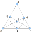
(a) Line-point Association

(b) Bipartite Representation

Figure 1: 2-dimensional Projective Geometry

To generate Projective Geometry corresponding to above Galois Field example($\mathbb{GF}$($2^{3}$)), the 2-dimensional projective plane, we treat each of the above non-zero element, the lone non-zero element of various 1-dimensional vector subspaces, as points of the geometry. Further, we pick various subfields(vector subspaces) of $\mathbb{GF}$($2^{3}$), and label them as various lines. Thus, the seven lines of the projective plane are {1, $\alpha$, $\alpha^{3}$ = $1+\alpha$}, {1, $\alpha^{2}$, $\alpha^{6}$ = $1+\alpha^{2}$}, {$\alpha$, $\alpha^{2}$, $\alpha^{4}$ = $\alpha^{2}+\alpha$}, {1,$\alpha^{4}$ = $\alpha^{2}+\alpha$, $\alpha^{5}$ = $\alpha^{2}+\alpha+1$}, {$\alpha$, $\alpha^{5}$ = $\alpha^{2}+\alpha+1$, $\alpha^{6}$ = $\alpha^{2}+1$}, {$\alpha^{2}$, $\alpha^{3}$ = $\alpha+1$, $\alpha^{5}$ = $\alpha^{2}+\alpha+1$} and {$\alpha^{3}$ = $1+\alpha$, $\alpha^{4}$ = $\alpha+\alpha^{2}$, $\alpha^{6}$ = $1+\alpha^{2}$}. The corresponding geometry can be seen as figures 1.

Let us denote the collection of all the $\mathbf{l}$-dimensional projective subspaces by $\mathbf{\Omega_{l}}$. Now, $\mathbf{\Omega_{0}}$ represents the set of all the points of the projective space, $\mathbf{\Omega_{1}}$ is the set of all lines, $\mathbf{\Omega_{2}}$ is the set of all planes and so on. To count the number of elements in each of these sets, we define the function

$$\phi(n,l,s)=\frac{(s^{n+1}-1)(s^{n}-1)\ldots(s^{n-l+1}-1)}{(s-1)(s^{2}-1)\ldots(s^{l+1}-1)}$$ (3)

Now, the number of $\mathbf{m}$-dimensional projective subspaces of ${\mathbb{P}}(d,\mathbb{F})$ is $\phi(d,m,s)$. For example, the number of points contained in ${\mathbb{P}}(d,F)$ is $\phi(d,0,s)$. Also, the number of $\mathbf{l}$-dimensional projective subspaces contained in an $\mathbf{m}$-dimensional projective subspace (where $0\leq l<m\leq d$) is $\phi(m,l,s)$, while the number of $\mathbf{m}$-dimensional projective subspaces containing a particular $\mathbf{l}$-dimensional projective subspace is $\phi(d-l-1,m-l-1,s)$.

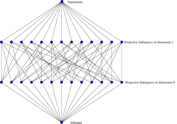
Figure 2: A Lattice Representation for 2-dimensional Projective Space

2.2 Projective Spaces as Lattices

It is a well-known fact that the lattice of subspaces in any projective space is a modular, geometric lattice [13]. A projective space of dimension 2 is shown in figure 2. In the figure, the top-most node represents the supremum, which is a projective space of dimension m in a lattice for $\mathbb{P}(\mathbf{m},\mathbb{GF}(\mathbf{q}))$. The bottom-most node represents the infimum, which is a projective space of (notational) dimension -1. Each node in the lattice as such is a projective subspace, called a flat. Each horizontal level of flats represents a collection of all projective subspaces of $\mathbb{P}(\mathbf{m},\mathbb{GF}(\mathbf{q}))$ of a particular dimension. For example, the first level of flats above infimum are flats of dimension 0, the next level are flats of dimension 1, and so on. Some levels have special names. The flats of dimension 0 are called points, flats of dimension 1 are called lines, flats of dimension 2 are called planes, and flats of dimension (m-1) in an overall projective space $\mathbb{P}(\mathbf{m},\mathbb{GF}(\mathbf{q}))$ are called hyperplanes.

2.3 Relationship between Projective Subspaces

Throughout the remaining paper, we will be trying to relate projective subspaces of various types. We define the following terms for relating projective subspaces.

Contained in

If a projective subspace X is said to be contained in another projective subspace Y, then the vector subspace corresponding to X is a vector subspace itself, of the vector subspace corresponding to Y. This means, the vectors contained in subspace of X are also contained in subspace of Y. In terms of projective spaces, the points that are part of X, are also part of Y. The inverse relationship is termed ‘contains’, e.g. “Y contains X”.

Reachable from

If a projective subspace X is said to be reachable from another projective subspace Y, then there exists a chain(path) in the corresponding lattice diagram of the projective space, such that both the flats, X and Y lie on that particular chain. There is no directional sense in this relationship.

2.4 Union of Projective Subspaces

Projective Spaces are point lattices. Hence the union of two projective subspaces is defined not only as set-theoretic union of all points(1-dimensional vector subspaces) which are part of individual projective subspaces, but also all the linear combinations of vectors in all such 1-dimensional vector subspaces. This is to ensure the closure of the newly-formed, higher-dimensional projective subspace. In the lattice representation, the flat corresponding to union is reachable from few more points, than those contained in the flats whose union is taken.

3 A Model for Computations Involved

3.1 The Computation Graph

The $\mathbf{0}$-dimensional subspaces of a $\mathbf{d}$-dimensional projective space (${\mathbb{P}}(d,\mathbb{F})$) projective space are called the points, and the $(\mathbf{d-1})$-dimensional subspaces are called the hyperplanes. Let $\mathbb{V}$ be the $(\mathbf{d+1})$-dimensional vector space corresponding to the projective space ${\mathbb{P}}(d,\mathbb{F})$. Then, as stated in the previous section, points will correspond to $\mathbf{1}$-dimensional vector subspaces of $\mathbb{V}$, and hyperplanes will correspond to $\mathbf{d}$-dimensional vector subspaces of $\mathbb{V}$. A bipartite graph is constructed from the point-hyperplane incidence relations as follows.

• Each point is mapped to a unique vertex in the graph. Each hyperplane is also mapped to a unique vertex of the graph.

• An edge exists between two vertices iff one of those vertices represents a point, the other represents a hyperplane and the $\mathbf{1}$-dimensional vector space corresponding to the point is contained in the $\mathbf{d}$-dimensional vector space corresponding to the hyperplane.

From the above construction, it is clear that the graph obtained will be bipartite; the vertices corresponding to points will form one partition and the vertices corresponding to the hyperplanes will form the other. Edges only exist between the two partitions. A point and hyperplane are said to be incident on each other if there exists an edge in between the corresponding vertices.

Points and hyperplanes form dual projective subspaces; the number of points contained in a particular hyperplane is given by $\phi(d-1,0,s)$ and the number of hyperplanes containing a particular point is given by $\phi(d-0-1,d-1-0-1,s)=\phi(d-1,d-2,s)$. After substitution into equation (3), it can easily be verified that $\phi(d-1,0,s)=\phi(d-1,d-2,s)$. Thus, the graph constructed is a regular balanced bipartite graph, with each vertex having a degree of $\phi(d-1,0,s)$.

In fact, many possible pairs of dual projective subspaces could be chosen to construct the graph, on which our folding scheme can be applied. Points and hyperplanes are the preferred choice because usually the applications require the graph to have a high degree. Choosing points and hyperplanes gives the maximum possible degree for a given dimension of projective space.

3.2 Description of Computations

The computations that can be covered using this design scheme are mostly applicable to the popular class of iterative decoding algorithms for error correcting codes, like LDPC or expander codes. A representation of such computation is generally available in the model described above, though it may go by some other domain-specific name such as Tanner Graph. The edges of such representative graph are considered as variables/datum of the system. A vertex of the graph represents computation of a constraint that needs to be satisfied by the variables corresponding to the edges(data) incident on the vertex. A edge-vertex incidence graph (EV-graph) is derived from the above graph. The EV-graph is bipartite, with one set of vertices representing variables and the other set of vertices representing the constraints. The decoding algorithm involves evaluation of all the constraints in parallel, and an update of the variables based on the evaluation. The vertices corresponding to constraints represent computations that are to be assigned to, and scheduled on certain processing units.

4 The Concept of Folding

Semi-parallel, or folded architectures are hardware-sharing architectures, in which hardware components are shared/overlaid for performing different parts of computation within a (single) computation. In its basic form, folding is a technique in which more than one algorithmic operations of the same type are mapped to the same hardware operator. This is achieved by time-multiplexing these multiple algorithm operations of the same type, onto single functional unit at system runtime.

The balanced bipartite PG graphs of various target applications perform parallel computation, as described in section 3.2. In its classical sense, a folded architecture represents a partition, or a fold, of such a (balanced) bipartite graph(see figure 3). The blocks of the partition, or folds can themselves be balanced or unbalanced; unbalanced folding entails no obvious advantage. The computational folding can be implemented after (balanced) graph partitioning in two ways. In the first way, that we cover in this paper, the within-fold computation is done sequentially, and across-fold computation is done parallely. This implies that many such sequentially operating folds are scheduled parallely. Such a more-popular scheme is generally called a supernode-based folded design, since a logical supernode is held responsible for operating over a fold. Dually, the across-fold computation can be made sequential by scheduling first node of first fold, first node of second fold, $\ldots$ sequentially on a single module. The within-fold computations, held by various nodes in the fold, can hence be made parallel by scheduling them over different hardware modules. Either way, such a folding is represented by a time-schedule, called the folding schedule. The schedule tells that in each machine cycle, which all computations are parallely scheduled on various functional units, and also the sequence of clusters of such parallel computations across machine cycles.

Figure 3: (Unevenly) Partitioned Bipartite DFG

4.1 Lattice Embedding

Projective Space lattices being modular lattices, it is also possible to exploit symmetry of (lattice) property reflection from a mid-way embedded level of flats from any two dual levels of flats which form a balanced bipartite graph based on their inter-reachability. For point-hyperplane bipartite graphs, this specialized scheme of folding is what we discuss here as one of the schemes. The other scheme involves usage of two dual mid-way embedded levels. Both these schemes are an example of the first type of folding: sequential within, and parallel across folds. We term such schemes as lattice embedding schemes, since the actual functional units(supernodes) are embedded at proper places(mid-way flats) in the corresponding PG lattice. An illustration of such folding is provided in figure 4.

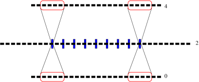
Figure 4: Folding PG Graph via Lattice Embedding

5 A Folding Scheme for $\mathbb{P}(5,\mathbb{GF}(2))$

In this section, we provide two schemes to demonstrate the possibilities of folding computations related to point hyperplane incidence graphs derived from 5-dimensional PG over $\mathbb{GF}(2)$, $\mathbb{P}(5,\mathbb{GF}(2))$. The schemes are summarized by following two propositions.

Proposition 1.

When considering computations based on the point-hyperplane incidence graph of $\mathbb{P}(5,\mathbb{GF}(2))$, it is possible to fold the computations and arrange a scheduling, that can be executed using 9 processing units and 9 dual port memories.

Proposition 2.

When considering computations based on the point-hyperplane incidence graph of $\mathbb{P}(5,\mathbb{GF}(2))$, it is possible to fold the computations and arrange a scheduling, that can be executed using 21 processing units and 21 dual port memories.

5.1 Proof of Propositions

5.1.1 Some Cardinalities of $\mathbb{P}(5,\mathbb{GF}(2))$ Lattice

We first present some important combinatorial figures associated with $\mathbb{P}(5,\mathbb{GF}(2))$. We will use these numbers in proving the functional correctness of the folded computations. For definition of $\phi(\cdot)$, refer equation 3.

• No. of points = No. of hyperplanes (4-dimensional projective subspace) = $\phi(5,0,2)=63$.

• No. of points contained in a particular hyperplane = $\phi(4,0,2)=31$

• No. of points contained in a line(1-dimensional projective subspace) = $\phi(1,0,2)=3$

• No. of points contained in a plane(2-dimensional projective subspace) = $\phi(2,0,2)=7$

• No. of points contained in a 3-dimensional projective subspace = $\phi(3,0,2)=15$

• No. of hyperplanes containing a particular plane = $\phi(5-2-1,4-2-1,2)=7$

• No. of hyperplanes containing a particular line = $\phi(5-1-1,4-1-1,2)=15$

• No. of hyperplanes containing a particular 3-dimensional projective subspace = $\phi(5-3-1,4-3-1,2)=3$

• No. of lines contained in a 3-dimensional projective subspace = $\phi(3,1,2)=35$

5.1.2 Lemmas for Proving Proposition 1

We prove the following lemmas, required to establish the feasibility of folding and scheduling using proposition 1.

Lemma 1.

The point set of a projective space of dimension 5 over $\mathbb{GF}(2)$ (represented by the non-zero elements of a vector space $\mathbb{V}$ over $\mathbb{GF}(2)$) can be partitioned into disjoint subsets such that each subset contains all the non-zero elements of a 3-dimensional vector subspace of $\mathbb{V}$. Thus, each such block of partition/subset represents a unique plane (2-dimensional projective subspace).

Proof.

The vector space $\mathbb{V}$ is represented by the field $\mathbb{GF}(2^{6})$ and has an order of 63. Since 3 is a divisor of 6, $\mathbb{GF}(2^{3})$ is a subfield of $\mathbb{GF}(2^{6})$. The multiplicative cyclic group of $\mathbb{GF}(2^{3})$ (of order 7) is isomorphic to a subgroup of the multiplicative cyclic group of $\mathbb{GF}(2^{6})$. Hence, we can perform a coset decomposition to generate 9 disjoint partitions of $\mathbb{V}$ into subsets such that each subset is a 3-dimensional vector space (-{0}), representing a 2-dimensional projective space i.e. a plane [2].

For details, assume that $\alpha$ is a generator for the multiplicative group of $\mathbb{GF}(2^{6})$. Then, $(1,\alpha^{9},\alpha^{18},\alpha^{27},\alpha^{36},\alpha^{45},$
$\alpha^{54})$ is the 7-element sub-group that we are looking for. The distinct cosets of this sub-group provide the partition that we need to generate disjoint projective subspaces. ∎

Corollary 2.

The above partitioning leads to partitioning of the set of hyperplanes (4-dimensional projective subspaces) as well. A (projective) plane can always be found that contains the intersection of all projective subspaces of the hyperplanes which belong to the same subset of hyperplanes belonging to a block of the partition, but itself is not contained in any hyperplane outside the subset. Here, intersection of projective subspace implies the intersection of their corresponding point sets.

Proof.

In $\mathbb{P}(5,\mathbb{GF}(2))$, each (projective) plane is contained in 7 hyperplanes. These hyperplanes are unique to the plane, since they represent the 7 hyperplanes that are common to the set of 7 points that form the plane. More explicitly, if two planes do not have any point contained in common, they will not be contained in any common hyperplane, and vice-versa. Thus, the 9 disjoint planes partition the hyperplane set into 9 disjoint subsets. ∎

Lemma 3.

In projective spaces over $\mathbb{GF}(2)$, any subset of points(hyperplanes) having cardinality of 4 or more has 3 non-collinear(independent) points(hyperplanes).

Proof.

The underlying vector space is constructed over $\mathbb{GF}(2)$. Hence, any 2-dimensional vector subspace contains the zero vector, and non-zero vectors of the form $\alpha\mathbf{a}+\beta\mathbf{b}$. Here, $\mathbf{a}$ and $\mathbf{b}$ are linearly independent one-dimensional non-zero vectors, and $\alpha$ and $\beta$ can be either 0 or 1, but not simultaneously zero:
$\alpha,\beta\;\in\;\mathbb{GF}(2):(\alpha\;=\;\beta)\;\neq\;0$.
Thus, any such 2-dimensional vector subspace contains exactly 3 non-zero vectors. Therefore, in any subset of 4 or more points of a projective space over $\mathbb{GF}(2)$ (which represent one-dimensional non-zero vectors in the corresponding vector space), at least one point is not contained in the 2-dimensional vector subspace formed by 2 randomly picked points from the subset. Thus in such subset, a further subset of 3 independent points(hyperplanes) i.e. 3 non-collinear vectors can always be found. ∎

Lemma 4.

In $\mathbb{P}(5,\mathbb{GF}(2))$, any point that does not lie on a plane $P_{1}$, but lies on some disjoint plane $P_{2}$, is contained in exactly 3 hyperplanes reachable from $P_{1}$. The vice-versa is also true. This lemma is used in section 5.1.3.

Proof.

If a point on plane $P_{2}$, which is not reachable from plane $P_{1}$, is contained in 4 or more hyperplanes(out of 7) reachable from plane $P_{1}$, then by lemma 3, we can always find a subset of 3 independent hyperplanes in this set of 4. In which case, the point will also be reachable from linear combination of these 3 independent hyperplanes, and hence to all the 7 hyperplanes which lie on plane 1. This contradicts the assumption that the point under consideration is not contained in plane $P_{1}$. The role of planes $P_{1}$ and $P_{2}$ can be interchanged, as well as roles of points and hyperplanes, to prove the remaining alternate propositions.

Hence if the point considered above is contained in exactly 3 hyperplanes reachable from $P_{1}$, then these 3 hyperplanes cannot be independent, following the same argument as above. If the 3 hyperplanes are not independent of one another, then it is indeed possible for such a point to be contained in 3 hyperplanes as follows. Let there be 2 disjoint planes $P_{1}$ and $P_{2}$ in $\mathbb{P}(5,\mathbb{GF}(2))$, whose set of independent points are represented by $\mathbf{(a,b,c)}$ and $\mathbf{(d,e,f)}$. Then, a point(e.g. $\mathbf{d}$) on $P_{2}$ is reachable from exactly 3 hyperplanes $\mathbf{(a,b,c,d,e)}$, $\mathbf{(a,b,c,d,f)}$ and $\mathbf{(a,b,c,d,(e+f))}$, which lie on $P_{1}$.

∎

From the above three lemmas, it is easy to deduce that a point reachable from a plane $P_{1}$ is further reachable from 7 hyperplanes through $P_{1}$, and 3 hyperplanes from each of the remaining 8 disjoint planes. The 9 disjoint planes can be found via construction in lemma 1. Thus, in a point-hyperplane graph made from $\mathbb{P}(5,\mathbb{GF}(2))$, the total degree of each point, 31, can be partitioned into 8*3 + 7 = 31 by using embedded disjoint projective planes, a result of paramount importance in our scheme. This is true for all points with respect to the planes that they are reachable from, and all hyperplanes with respect to the plane they contain. This symmetry is used to derive a conflict free memory access schedule and its corresponding data distribution scheme.

5.1.3 Proof of Proposition 1

We prove now, the existence of folding mentioned in proposition 1 constructively, by providing an algorithm below for folding the graph, as well as scheduling computations over such folded graph.

We have shown above in lemma 1 that we can partition the set of points into 9 disjoint subsets (each corresponding to a plane). The algorithm for partitioning is based on [2]. Also, there is a corresponding partitioning of the hyperplane set. Let the planes assigned to the partitions be $P_{1},P_{2}\ldots,P_{9}$.We will assign a processing unit (system resource) to each of the planes. Let us abuse notation and call the processing units by the name corresponding to the plane assigned to them. We add a commercially-off-the-shelf available dual port memory $M_{i}$ to each processing unit $P_{i}$, to store computational data. We then provide a proven schedule that avoids memory conflicts. The distribution of data among the memories follows from the schedule. Both these issues are addressed below.

For the computations we are considering, the processing units perform computations on behalf of the points as well as the hyperplanes. The data symbols are represented by the edges of the bipartite graph. The overall computation is broken into two phases. Phase 1 corresponds to the point vertices performing the computations, using the edges, and updating the necessary data symbols. Phase 2 corresponds to the hyperplanes performing the computations, and updating the necessary data symbols.

The data distribution among the memories local to the 9 processing units ($M_{0},M_{1}\ldots,M_{8}$), and subsequent scheduling, is done as follows.

• In Phase 1, processing unit $P_{i}$ performs the computations corresponding to the points that are contained in the plane $P_{i}$, in a sequential fashion. For each of the 7 points contained in the plane $P_{i}$, there will be 7 units of data corresponding to 7 hyperplanes containing plane $P_{i}$. Thus, 49 units of data corresponding to them will be stored in $M_{i}$. In addition to this, $M_{i}$ will further store 3 units of data for each of the 56 remaining points not contained in $P_{i}$. These 3 units of data correspond to the incidence of each of the points not contained in $P_{i}$ with some 3 hyperplanes containing the plane $P_{i}$; see lemma 4.

  Lemma 5.

  The distribution of data as described above leads to a conflict-free memory-access pattern, when all the processing units are made to compute in parallel same computation but on different data.

  Proof.

  Suppose processing unit $P_{1}$ is beginning the computation cycle corresponding to some point $\mathbf{a}$. It needs to fetch data from the memories, perform some computation and write back the output of the computation. First, it collects the 7 units of data corresponding to $\mathbf{a}$ in $M_{1}$. This corresponds to the edges that exist between point $\mathbf{a}$ and the hyperplanes that contain plane $P_{1}$. Next, it fetches 3 units of data from each of the remaining 8 memories. This consists of the edges between $\mathbf{a}$ and the 3 hyperplanes from each of the planes not containing $\mathbf{a}$. Thus, $7+3*8=31$ units of data will be fetched for $\mathbf{a}$. We have all the 9 processing units working in parallel, and each of them follows the same schedule.

  For processing unit $P_{i}$, first, 7 units of data from $M_{i}$ are fetched locally. Further, 3 units of data are fetched from each $M_{(i+j)mod9}$, $\mathbf{j}$ going from 1 to 8. Thus, during the time when $P_{0}$ is accessing $M_{1}$, $P_{1}$ will be accessing $M_{2}$, and so on till we reach $P_{8}$ which will be accessing $M_{0}$. In this fashion, no two processing units will be trying to access the same memory at the same time i.e. no memory access conflicts will occur. ∎

  The writing of the output is done with the same schedule. If dual port memories are used, we can overlap the writing of the output of one point using one port, with the reading of the input of the next point using the other port.

• In Phase 2, processing unit $P_{i}$ performs the computation corresponding to the hyperplanes that contain plane $P_{i}$. If the data is distributed as explained in the previous point, then $M_{i}$ already contains all the data required for the hyperplanes containing plane $P_{i}$. In this case, the processing unit communicates only with its own memory and performs the computation.

For above data distribution, the address generator circuit in Phase 1 is just a counter, while in Phase 2 it becomes a look up table. The address generation circuits are incorporated within the processing unit itself. As can be observed from the above discussion, while scheduling different computations on the same physical processing unit, data does not need any internal or external shuffling across memories associated with other processing units. This, along with complete conflict freedom in memory accesses, saves the entire significant overhead of general folding schemes, which includes shuffling of data in between scheduling of two folds. Thus one achieves the best theoretically possible throughput in such designs.

5.1.4 Lemmas for Proving Proposition 2

We now move on to proving Proposition 2. Proposition 2 represents moving away from chosing the exact mid-way level of flats in PG lattice, to multiple choices of two dual levels of flats, for folding purposes. Thus it is a generalization of Proposition 1.

Lemma 6.

The point set of a projective space of dimension 5 over $\mathbb{GF}(2)$ (represented by the non-zero elements of a vector space $\mathbb{V}$ of dimension 6 over $\mathbb{GF}(2)$) can be partitioned into disjoint subsets such that each subset contains the non-zero elements of a 2-dimensional vector subspace of $\mathbb{V}$. Each subset/block of the partition represents a unique line (1-dimensional projective subspace).

Proof.

The proof is very similar to lemma 1. As before, $\mathbb{V}$ is represented by $\mathbb{GF}(2^{6})$ and since 2 divides 6, $\mathbb{GF}(2^{2})$ is a subfield. Thus $\mathbb{V}$ can be partitioned into disjoint vector subspaces(-{0}) of dimension 2 each (using coset decomposition [2]). Each of these vector subspaces represents a 1-dimensional projective subspace (line), and contains 3 points. ∎

Corollary 7.

The dual of above partitioning partitions the set of hyperplanes (4-dimensional projective subspaces) into disjoint subsets of 3 hyperplanes each. A unique 3-dimensional projective subspace can always be found that is contained in all the 3 hyperplanes of one such subset, and none from any other subset.

Proof.

By duality of projective geometry, it follows that we can partition the set of hyperplanes into disjoint subsets of 3 each, such that each subset represents a unique 3-dimensional projective subspace. This can be achieved by performing a suitable coset decomposition of the dual vector space. ∎

Thus, we can partition the set of 63 points into 21 sets of 3 points each. In this way, we have a one-to-one correspondence between a point and the line that contains it. We now provide certain lemmas, that will be needed to prove theorem 11 later, which establishes the existence of a conflict-free schedule.

Lemma 8.

The union of two disjoint lines(1-dimensional projective subspaces) in $\mathbb{P}(5,\mathbb{GF}(2))$ leads to a 3-dimensional projective subspace.

Proof.

Let the two disjoint lines be $L_{1}$ and $L_{2}$. Being disjoint, they have no points contained in common.

Each line, being a 2-dimensional vector space contains exactly two independent points. Thus, two disjoint lines will contain 4 independent points. Taking a union, we get all possible linear combinations of the 4 independent points which corresponds to a 4-dimensional vector space(lets call it $T_{12}$). The 4 independent points have been taken from the points of the 6-dimensional vector space $\mathbb{V}$, used to describe the projective space. Thus, the 4-dimensional vector space, made up of all the linear combinations of the 4 points, is a vector subspace of $\mathbb{V}$.

Being a 4-dimensional vector subspace of $\mathbb{V}$, $T_{12}$ represents a 3-dimensional projective subspace. ∎

Lemma 9.

For $\mathbb{P}(5)$, let $\mathbb{L}=\{L_{0},L_{1},\ldots,L_{20}\}$ be the set of 21 disjoint lines obtained after coset decomposition of $\mathbb{V}$. Let $T_{ij}$ be the 3-dimensional projective space obtained after taking the union of the lines $L_{i},L_{j}$, both taken from the set $\mathbb{L}$. Then, any line $L_{k}$ from the set $\mathbb{L}$, is either contained in $T_{ij}$ or does not share any point with $T_{ij}$. Specifically, if it shares one point with $T_{ij}$, then it shares all its points with $T_{ij}$.

Proof.

Let $\alpha$ be the generator of the cyclic multiplicative group of $\mathbb{GF}(2^{6})$. Then the points of the projective space will be given by $\{\alpha^{0},\alpha^{1},\ldots,\alpha^{62}\}$ and for any integer $\mathbf{i}$, $\alpha^{i}=\alpha^{(i\;mod\;63)}$.

The lines of a projective space are equivalent to 2-dimensional vector subspaces. After the relevant coset decomposition of $\mathbb{GF}(2^{6})$, as per lemma 6, without loss of generality, we can generate a correspondence between lines of $\mathbb{L}$ and the cosets as follows.

$$L_{0}\equiv\{\alpha^{0},\alpha^{21},\alpha^{42}\}$$

$$L_{1}\equiv\{\alpha^{1},\alpha^{22},\alpha^{43}\}$$

$$L_{2}\equiv\{\alpha^{2},\alpha^{23},\alpha^{44}\}$$

$$\vdots$$

$$L_{19}\equiv\{\alpha^{19},\alpha^{40},\alpha^{61}\}$$

$$L_{20}\equiv\{\alpha^{20},\alpha^{41},\alpha^{62}\}$$

Now, $L_{i}\equiv\{\alpha^{i},\alpha^{i+21},\alpha^{i+42}\}$, where, $\mathbf{i}+21\cong((\mathbf{i}+21)\;mod\;63)$ and $\mathbf{i}+42\cong((\mathbf{i}+42)\;mod\;63)$.

Similarly, $L_{j}\equiv\{\alpha^{j},\alpha^{j+21},\alpha^{j+42}\}$

Now, $T_{ij}$ is given by the union of $L_{i},L_{j}$. Thus, $T_{ij}$ contains all possible linear combinations of the points of $L_{i}$ and $L_{j}$. Let us divide the points of $T_{ij}$ into two parts:

1. The first part $X_{1}$ is given by the 6 points contained in $L_{i}$ and $L_{j}$.

2. The second part $X_{2}$ contains 9 points obtained by the linear combinations of the form $\mathbf{a}\alpha^{u}+\mathbf{b}\alpha^{v}$, where $\alpha^{u}\in L_{i}$ and $\alpha^{v}\in L_{j}$ and $\mathbf{a,b}$ take the non-zero values of $\mathbb{GF}(2)$, i.e. $\mathbf{a=b=1}$.

Consider any line $L_{k}\in\mathbb{L}$.

• Case 1:
  If $\mathbf{k}=\mathbf{i}$ or $\mathbf{k}=\mathbf{j}$, then by the given construction, it is obvious that $L_{k}\subset T_{ij}$ and the lemma holds.

• Case 2:
  Here, $\mathbf{k}\neq\mathbf{i,j}$
  We have, $L_{k}\equiv\{\alpha^{k},\alpha^{k+21},\alpha^{k+42}\}$. Also, $L_{k}\in\mathbb{L}$ and $\mathbf{k}\neq\mathbf{i,j}$ implies that $L_{k}$ is disjoint from $L_{i}$ and $L_{j}$. Thus, it has no points contained in common with $L_{i}$ and $L_{j}$.

  Since $L_{k}$ has no points contained in common with $L_{i}$ and $L_{j}$, it cannot have any points in common with the set of points $X_{1}$ of $T_{ij}$ defined above.

  Now, we will prove that if $L_{k}$ has even a single point in common with the set of points $X_{2}$ defined in point 2 above, then it has all its points in common with the set $X_{2}$ which implies that $L_{k}\subset T_{ij}$. If no points are in common, then $L_{k}$ is not contained $T_{i,j}$ as required by the lemma.

  Without loss of generality, let $\alpha^{k}=\alpha^{u}+\alpha^{v}$ for some $\alpha^{u}\in L_{i}$ and $\alpha^{v}\in L_{j}$.

  From the coset decomposition given above, it is clear that if $\alpha^{k}\in L_{k}$, then $\alpha^{k+21}\in L_{k}$, and $\alpha^{k+42}\in L_{k}$. Here again, $\mathbf{k}+21\cong((\mathbf{k}+21)\;mod\;63)$ and $\mathbf{k}+42\cong((\mathbf{k}+42)\;mod\;63)$.

  Since $\alpha$ is a generator of a multiplicative group, $\alpha^{k+21}=\alpha^{k}.\alpha^{21}$, and $\alpha^{k+42}=\alpha^{k}.\alpha^{42}$.

  Also, one of the fundamental properties of finite fields states that the elements are abelian with respect to multiplication and addition and the multiplication operator distributes over addition, i.e.

  $$\mathbf{a.(b+c)=(b+c).a=a.b+a.c=b.a+c.a}$$ (4)

  where $\mathbf{a,b,c}$ are elements of the field.

  Consider, $\alpha^{k+21}$, We have,

  $$\alpha^{k+21} = \alpha^{k}.\alpha^{21}$$ (5)

  $$\Longrightarrow\alpha^{k+21} = (\alpha^{u}+\alpha^{v}).\alpha^{21}$$ (6)

  $$\Longrightarrow\alpha^{k+21} = \alpha^{u}.\alpha^{21}+\alpha^{v}.\alpha^{21}$$ (7)

  $$\Longrightarrow\alpha^{k+21} = \alpha^{u+21}+\alpha^{v+21}$$ (8)

  Here, (7) follows because of (4) and, as usual, the addition in the indices is taken modulo 63.

  Since, $\alpha^{u}\in L_{i}$ and $\alpha^{v}\in L_{j}$, from the coset decomposition scheme, we have, $\alpha^{u+21}\in L_{i}$ and $\alpha^{v+21}\in L_{j}$. Thus, $\alpha^{u+21}\in T_{ij}$ and $\alpha^{v+21}\in T_{ij}$. And finally, $(\alpha^{u+21}+\alpha^{v+21})\in T_{i,j}$ which has the straightforward implication that $\alpha^{k+21}\in T_{ij}$.

  Analogous arguments for $\alpha^{k+42}$ prove that $\alpha^{k+42}\in T_{ij}$. Thus, all three points of $L_{k}$ are contained in $T_{i.j}$ and $L_{k}\subset T_{i,j}$.

  The arguments above show that any line $L_{k}\in\mathbb{L}$ either is completely contained in $T_{ij}$ or has no intersecting points with it. For the sake of completeness, we present the points in $T_{ij}$ so that is easy to “see” the lemma:

  $$T_{ij}=\left[\begin{array}[]{c c c}\alpha^{i}&\alpha^{i+21}&\alpha^{i+42}\\ \alpha^{j}&\alpha^{j+21}&\alpha^{j+42}\\ \alpha^{j}+\alpha^{i}&\alpha^{j+21}+\alpha^{i}&\alpha^{j+42}+\alpha^{i}\\ \alpha^{j}+\alpha^{i+21}&\alpha^{j+21}+\alpha^{i+21}&\alpha^{j+42}+\alpha^{i+21}\\ \alpha^{j}+\alpha^{i+42}&\alpha^{j+21}+\alpha^{i+42}&\alpha^{j+42}+\alpha^{i+42}\\ \end{array}\right]$$

∎

Lemma 10.

Given the set $\mathbb{L}$ of 21 disjoint lines that cover all the points of $\mathbb{P}(5,\mathbb{GF}(2))$, pick any $L_{i}\in\mathbb{L}$ and take its union with the remaining 20 lines in $\mathbb{L}$ to generate 20 3-dimensional projective subspaces. Of these 20, only 5 distinct 3-dimensional projective subspaces will exist.

Proof.

Any 3-dimensional projective subspace has 3 hyperplanes containing it, refer corollary 7. If a line is contained in a 3-dimensional projective subspace, then it is contained in all the 3 hyperplanes, that contain that 3-dimensional projective subspace.

Also, if a line is not contained in a 3-dimensional projective subspace, it is not contained in any of the hyperplanes, that contain it. This is because:

$$dim(L_{1}\cup T_{1})=dim(L_{1})+dim(T_{1})-dim(L_{1}\cap T_{1})$$

$$dim(L_{1})=2\;,\;dim(T_{1})=4$$

$$dim(L_{1}\cap T_{1})=0$$

$$\Longrightarrow dim(L_{1}\cup T_{1})=6$$

where $L_{1}$ is the line, and $T_{1}$ is the 3-dimensional projective subspace not containing the line. A hyperplane is a 5-dimensional vector subspace. So, if $dim(L_{1}\cup T_{1})>5$, $L_{1}$ is not contained in any hyperplane containing $T_{1}$.

Let $T_{ij}$ and $T_{jk}$ be two 4-dimensional vector subspaces of $\mathbb{V}$ that represent two 3-dimensional projective subspaces. Then, $dim(T_{ij})=dim(T_{jk})=4$. Also,

$$dim(T_{ij}\cup T_{jk})=dim(T_{ij})+dim(T_{jk})-dim(T_{ij}\cap T_{jk})$$

It is easy to see that by virtue of base Galois field being $\mathbb{GF}(2)$, $T_{ij}$ and $T_{jk}$ have 0,1 or 3 common hyperplanes. No other case is possible. If they have 3 common hyperplanes, then $T_{ij}$ = $T_{jk}$. This implies that $dim(T_{ij}\cap T_{jk})=4$.

If they have one hyperplane in common, the 5-dimensional vector subspace corresponding to that hyperplane must contain both the 4-dimensional vector subspaces. This is possible iff $dim(T_{ij}\cup T_{jk})=5$, which in turn, by rank arguments, implies $dim(T_{ij}\cap T_{jk})=3$.

If they have no hyperplane in common, then $dim(T_{ij}\cup T_{jk})=6$ which again, by rank arguments, implies $dim(T_{ij}\cap T_{jk})=2$.

Consider the union of line $L_{i}$ with $L_{j}\in\mathbb{L},j\neq i$. By Lemma 8, the union generates a 3-dimensional projective space. Lets call it $T_{ij}$. Similarly, let the union of line $L_{i}$ with $L_{k}\in\mathbb{L},k\neq i,j$ be called $T_{ik}$.

By lemma 9, either $L_{k}\subset T_{ij}$ or $L_{k}\cap T_{ij}=0$.

If $(L_{i},L_{k})\subset T_{ij}$, then $T_{ik}$=$T_{ij}$.

If $L_{k}\cap T_{ij}=0$, then $T_{ik}$ is distinct from $T_{ij}$. Since exactly 3 hyperplanes contain a 3-dimensional projective subspace $T_{ik}$, which in turn contains $L_{i}$, 3 new hyperplanes reachable from $L_{i}$ get discovered as and when we get another distinct 3-dimensional projective subspace. Moreover, $dim(T_{ij}\cap T_{ik})=2$, which implies that $T_{ij}$ and $T_{ik}$ do not share any hyperplanes.

Applying this argument iteratively for the 20 3-dimensional projective subspaces we see that a maximum of $\mathbf{5}$ distinct 3-dimensional projective subspaces can be generated, each of which gives a cardinality of 3 hyperplanes to $L_{i}$, thus making 15 hyperplanes.

Each 3-dimensional projective subspace, e.g. $T_{ij}$ contains 15 points and hence, it can contain a maximum of 5 disjoint lines. One of them is $L_{i}$, and another 4 need to be accounted for. So, when the union of $L_{i}$ is taken with the remaining 20 lines, a maximum of 4 lines, out of these 20 lines, can give rise to same 3-dimensional projective subspace, $T_{ij}$. This implies that a minimum of 20/4 = $\mathbf{5}$ 3-dimensional projective subspaces can be generated from the remaining 20 lines.

Since a maximum and minimum of 5 3-dimensional projective subspaces can be generated, exactly 5 distinct 3-dimensional projective subspaces are generated. Moreover, none of these subspaces share any hyperplanes. ∎

5.1.5 Proof of Proposition 2

The main theorem behind the construction of schedule mentioned in proposition 2, is as following.

Theorem 11.

In $\mathbb{P}(5,\mathbb{GF}(2))$, given a set of 21 disjoint lines (1-dimensional projective subspaces) that cover all the points, a set of 21 disjoint 3-dimensional projective subspaces can be created such that they cover all the hyperplanes. Here, hyperplane covering implies that each hyperplane of $\mathbb{P}(5,\mathbb{GF}(2))$ contains, or is reachable in the lattice to, at least one of the 21 disjoint 3-dimensional projective subspaces as its subspace. In this case, each point attains its cardinality of 31 reachable hyperplanes in $\mathbb{P}(5,\mathbb{GF}(2))$, in the following manner:

1. It is reachable from 3 hyperplanes each, via 5 3-dimensional projective subspaces that contain the line corresponding to it, as per the partition in 6.

2. It is reachable from 1 hyperplane each, via the remaining 16 3-d projective subspaces that necessarily cannot contain the line corresponding to it.

The dual argument with the roles of points and hyperplanes interchanged also holds.

Proof.

Generate the set of 21 disjoint lines $\mathbb{L}$ according to the coset decomposition corresponding to the subgroup isomorphic to $\mathbb{GF}(2^{2})$. We choose this subgroup as the canonical subgroup mentioned in Lemma 9, i.e. {$\alpha^{0}$, $\alpha^{21}$, $\alpha^{42}$}.

Choose any line $L_{i}$ from this set and take its union with the remaining 20 lines in the set to generate 5 distinct 3-dimensional projective subspaces(as proved in lemma 10). Call these projective subspaces $T_{1},T_{2},\ldots,T_{5}$. Choose 5 distinct lines, each NOT equal to $L_{i}$, to represent each of these projective subspaces. Such a choice exists by lemma 8. Pick the line representing $T_{1}$, and take its union with the other 4 lines to generate 4 new 3-dimensional projective subspaces. Choose 4 more lines(distinct from the 5 lines used earlier), to represent these 4 new projective subspaces. Again, such distinct lines exist by lemma 8, and there are overall 21 distinct lines. Pick another line from $T_{1}$ (not equal to the previously used lines), and take its union with the 4 newly chosen lines to form yet more 4 new 3-dimensional projective subspaces. Repeat this process 2 more times, till one gets 21 different 3-d projective subspaces, each contributing 3 distinct hyperplanes to $L_{i}$.

The following facts hold for the partitions of hyperplanes and points implied by the above generation process.

1. Each line in the set $\mathbb{L}$ is contained in 5 3-d projective subspaces, and each 3-dimensional projective subspace contains 5 lines from the set $\mathbb{L}$.

2. A point in a line is reachable from 3 hyperplanes via every 3-d projective subspace that contains the line, and 1 hyperplane via every projective subspace that doesn’t contain the line. In the latter case, if the 3-dimensional projective subspace doesn’t contain the line, it doesn’t contain the point. Hence, the projective subspace will only contribute one hyperplane corresponding to the union of the point with the 3-d projective subspace.

From the above facts, all the points of the theorem follow. The dual argument holds in exactly the same way. One could have started with a partition of 3-dimensional projective subspaces and generated lines by completely working in the dual vector space and using the exact same arguments. Hence, there are two ways of folding for each partition of $\mathbb{V}$ into disjoint lines. ∎

To prove Proposition 2, we use lemmas 6, 8, 9, 10 and the above main theorem. For a system based on point-hyperplane graph of $\mathbb{P}(5,\mathbb{GF}(2))$, the graph can be folded easily, from theorem 11. A scheduling similar to the one used for Proposition 1 can then be developed as following.

We begin by assigning one processing unit to every line of the disjoint set of 21 lines. Each processing unit has an associated local memory. After the 3-dimensional projective subspaces have been created as explained above, we can assign a 3-d projective space to each of the memories. The computation is again divided into two phases. In phase 1, the points on a particular line are scheduled on the processing units corresponding to that line in a sequential manner. A point gets 3 data units from a memory if the 3-dimensional projective space corresponding to that memory contains the line, otherwise it gets 1. In phase 2, the memory already has data corresponding to the hyperplanes that contain the 3-dimensional projective subspace representing the memory and the communication is just between the processing unit and its own memory. The output write-back cycles follow the schedule of input reads in both phases. It is straightforward to prove, on lines of Lemma 5, that the above distribution of data again leads to a conflict-free memory-access pattern, when all the processing units are made to compute in parallel same computation but on different data.

6 Generalization of Folding Scheme to Arbitrary Projective Geometries

In previous section, we gave complete construction of graph folding, and corresponding scheduling for example of $\mathbb{P}(5,\mathbb{GF}(2))$. In this section, we generalize above propositions for projective geometries of arbitrary dimension $\mathbf{m}$, and arbitrary non-binary Galois Field $\mathbb{GF}(\mathbf{q})$. The generalization is carried out for cases where $(\mathbf{m+1})$ is not a prime number. By extending the Prime Number Theorem to integer power of some fixed number, it is expected that not many cases(values of q) are left out by doing such restricted coverage.

A $\mathbb{P}(\mathbf{m},\mathbb{GF}(\mathbf{q}))$ is represented using the elements of a vector space $\mathbb{V}$ of dimension $(\mathbf{m+1})$ over $\mathbb{GF}(\mathbf{q})$. If $(\mathbf{m+1})$ is not prime, it can be factored into non-trivial prime factors $\mathbf{p_{1},p_{2},p_{3},\ldots,p_{n}}$ such that
$\mathbf{p_{1}\times p_{2}\times\ldots\times p_{n}}=\left(\mathbf{m+1}\right)$. The dimensions of these projective subspaces vary from $\mathbf{1}$ to $\left(\mathbf{\frac{m-1}{2}}\right)$, and the dimensions of the corresponding vector subspaces of $\mathbb{V}$ vary from $\mathbf{2}$ to $\left(\mathbf{\frac{m+1}{2}}\right)$. The points are the $\mathbf{0}$-dimensional projective subspaces (represented by the 1-dimensional vector subspaces of $\mathbb{V}$) and the hyperplanes are the $(\mathbf{m-1})$ dimensional projective subspaces.

It is convenient to describe the folding scheme in two separate cases.

6.1 Folding for Geometry with Odd dimension

Suppose $(\mathbf{m+1})$ is even. We prove the following lemmas.

Lemma 12.

(Generalization of Lemma 1) In $\mathbb{P}(\mathbf{m},\mathbb{GF}(\mathbf{q}))$ with odd $\mathbf{m}$, the set of points, which has cardinality $\left(\frac{q^{m+1}-1}{q-1}\right)$, can be partitioned into disjoint subsets. Each block of this partition is a vector subspace having dimension $\left(\frac{m+1}{2}\right)$, and contains $\left(\frac{q^{\frac{(m+1)}{2}}-1}{q-1}\right)$ points each.

Proof.

Let the vector space $\mathbb{V}$, corresponding to $\mathbb{P}(\mathbf{m},\mathbb{GF}(\mathbf{q}))$, be represented by $\mathbb{GF}(q^{m+1})$. Since $(\mathbf{m+1})$ is even, $\left(\frac{m+1}{2}\right)$ divides $(\mathbf{m+1})$. Hence, $\mathbb{GF}(q^{\frac{m+1}{2}})$ is a sub-field of $\mathbb{GF}(q^{m+1})$. The multiplicative cyclic group of $\mathbb{GF}(q^{\frac{m+1}{2}})$ is isomorphic to a subgroup of the multiplicative cyclic group of $\mathbb{GF}(q^{m+1})$. Hence, we can again perform a coset decomposition to generate disjoint blocks of partition of corresponding vector space, $\mathbb{V}$, into subsets. Each such subset is a $\left(\frac{m+1}{2}\right)$-dimensional vector subspace (-{0})(say, $\mathbf{S_{i}}$), representing a $\left(\frac{m-1}{2}\right)$-dimensional projective space i.e. a plane [2]. By property of vector subspaces, if $\mathbf{x\in S_{i}}$ then $\lambda\cdot\mathbf{x\in S_{i}}$, where $\lambda\in\mathbb{GF}(\mathbf{q})$. Since each point represents an equivalence class of vectors, except 0, a projective subspace of dimension $\left(\frac{m-1}{2}\right)$, corresponding to each partitioned vector subspace, contains exactly $\left(\frac{q^{\frac{(m+1)}{2}}-1}{q-1}\right)$ points. ∎

Lemma 13.

(Generalization of Corollary 2) In $\mathbb{P}(\mathbf{m},\mathbb{GF}(\mathbf{q}))$ with odd $\mathbf{m}$, the set of hyperplanes, which has cardinality $\left(\frac{q^{m+1}-1}{q-1}\right)$, can be partitioned into disjoint subsets. Each block of this partition is a vector subspace having dimension $\left(\frac{m+1}{2}\right)$, and contains $\left(\frac{q^{\frac{(m+1)}{2}}-1}{q-1}\right)$ hyperplanes each.

Proof.

Because of duality of points and hyperplanes, there are an equal number of hyperplanes containing each $\left(\frac{m+1}{2}-1\right)$-dimensional projective subspace. Further, the set of such subspaces together covers all the hyperplanes of $\mathbb{P}(\mathbf{m},\mathbb{GF}(\mathbf{q}))$. Here, hyperplane covering implies that each hyperplane of $\mathbb{P}(\mathbf{m},\mathbb{GF}(\mathbf{q}))$ contains, or is reachable in the lattice to, at least one of the chosen disjoint $\left(\frac{m-1}{2}\right)$-dimensional projective subspaces as its subspace. Moreover, since we have a disjoint partition of points, there will exist a corresponding disjoint partition of hyperplanes. The number of such partitions can easily be seen to be $\left(\frac{q^{m+1}-1}{q^{\frac{(m+1)}{2}}-1}\right)$. ∎

The following theorem extends the partitioning portion of Proposition 1, as detailed in its proof.

Theorem 14.

Each point of $\mathbb{P}(\mathbf{m},\mathbb{GF}(\mathbf{q}))$ with odd $\mathbf{m}$ is contained in $\left(\frac{q^{\frac{(m+1)}{2}}-1}{q-1}\right)$ hyperplanes belonging to a unique block of the partition that contains this point, and $\left(\frac{q^{m}-q^{\frac{(m+1)}{2}}}{q-1}\right)$ hyperplanes from remaining blocks of partition, that do not contain this point.

Proof.

By equation 3, each point has a total of $\left(\frac{q^{m}-1}{q-1}\right)$ hyperplanes containing it. By putting lemmas 12 and 13 together, one can see that it is contained in $\left(\frac{q^{\frac{(m+1)}{2}}-1}{q-1}\right)$ hyperplanes belonging to the partition that contains this point. It is also contained in $\left(\frac{q^{m}-q^{\frac{(m+1)}{2}}}{q-1}\right)$ hyperplanes belonging to the remaining $\left(\frac{q^{m+1}-1}{q^{\frac{(m+1)}{2}}-1}\right)-1$ = $\mathbf{q^{\frac{(m+1)}{2}}}$ partitions in the following manner, using the two lemmas below.

Lemma 15.

(Generalization of Lemma 3) In $\mathbb{P}(\mathbf{m},\mathbb{GF}(\mathbf{q}))$, from any set of $\left(\frac{q^{\frac{(m-1)}{2}}-1}{q-1}+\mathbf{1}\right)$ points(hyperplanes), it is possible to find $\left(\frac{m-1}{2}+1\right)$ = $\left(\frac{m+1}{2}\right)$ independent points(hyperplanes).

Proof.

As mentioned earlier via lemma 13, each block of the partition of hyperplane set is covered by a vector subspace of dimension $\left(\frac{m+1}{2}\right)$. This representative vector subspace, in turn, is formed by $\left(\frac{m+1}{2}\right)$ independent points and all their linear combinations contained in it, using coefficients from $\mathbb{GF}(\mathbf{q})$. The total number of points contained in a $\left(\frac{m-1}{2}\right)$ dimensional vector space, based on $\left(\frac{m-1}{2}\right)$ independent points, is $\left(\frac{q^{\frac{(m-1)}{2}}-1}{q-1}\right)$. Therefore, in any set of $\left(\frac{q^{\frac{(m-1)}{2}}-1}{q-1}+\mathbf{1}\right)$ points, it is possible to find $\left(\frac{m-1}{2}+1\right)$ = $\left(\frac{m+1}{2}\right)$ independent points.

By duality in PG lattice, it is straightforward to prove that in any set of $\left(\frac{q^{\frac{(m-1)}{2}}-1}{q-1}+\mathbf{1}\right)$ hyperplanes, it is possible to find $\left(\frac{m-1}{2}+1\right)$ = $\left(\frac{m+1}{2}\right)$ independent hyperplanes as well. ∎

Lemma 16.

(Generalization of lemma 4) Any point that does not lie in a $\left(\frac{m-1}{2}\right)$ dimensional projective subspace is reachable from exactly $\left(\frac{q^{\frac{(m-1)}{2}}-1}{q-1}\right)$ hyperplanes through that projective subspace, which is contained in $\left(\frac{q^{\frac{(m+1)}{2}}-1}{q-1}\right)$ hyperplanes overall.

Proof.

If that point is reachable from any more hyperplanes than $\left(\frac{q^{\frac{(m-1)}{2}}-1}{q-1}\right)$, then by lemma 15, we could find $\left(\frac{m+1}{2}\right)$ independent hyperplanes reachable from both this point as well as a $\left(\frac{m-1}{2}\right)$ dimensional projective subspace. A $\left(\frac{m-1}{2}\right)$ dimensional projective subspace contains exactly $\left(\frac{m+1}{2}\right)$ independent points and hyperplanes. Hence the presence of $\left(\frac{m+1}{2}\right)$ independent hyperplanes containing a particular $\left(\frac{m-1}{2}\right)$ dimensional projective subspace implies that all the $\left(\frac{m+1}{2}\right)$ independent points also contained in the same subspace, and their linear combinations, are exactly the points that are reachable from such set of hyperplanes. This contradicts the fact that the original point was not one of the $\left(\frac{m+1}{2}\right)$ independent points reachable from the $\left(\frac{m-1}{2}\right)$ dimensional projective subspace.

If that point is contained in any less hyperplanes, then the point would not be reachable from the established number of hyperplanes in the above partition, as governed by its degree. From the equations below, it is easy to see that even if 1 partition not containing the considered point contributes even 1 hyperplane less towards degree of the considered point, the overall degree of the point in the bipartite graph cannot be achieved.

Hyperplanes from partitions not containing the point $$= \left(\frac{q^{\frac{(m-1)}{2}}-1}{q-1}\right)*q^{\frac{(m+1)}{2}}$$

$$= \left(\frac{q^{m}-q^{\frac{(m+1)}{2}}}{q-1}\right)$$

Total degree $$= \left(\frac{q^{\frac{(m+1)}{2}}-1}{q-1}\right)\mbox{\normalsize{(from partition containing the point)}}+\left(\frac{q^{m}-q^{\frac{(m+1)}{2}}}{q-1}\right)$$

$$= \left(\frac{q^{m}-1}{q-1}\right)$$

as required

∎

Putting together these two lemmas, we arrive at the desired conclusion for theorem 14. ∎

Given the above construction, it is easy to develop a folding architecture and scheduling strategy by extending the scheduling for $\mathbb{P}(5,\mathbb{GF}(2))$ in section 5.1.3 in a straightforward way. One processing unit is once again assigned to each of the disjoint partitions of points. Using a memory of size $\left(\frac{q^{m}-1}{q-1}\right)$ collocated with the processing unit, it is again possible to provably generate a conflict-free memory access pattern, by extending Lemma 5. We omit the details of the scheduling strategy, since it is a simple extension of the strategies discussed earlier for a 5-dimensional projective space.

6.2 Folding for Geometry with Even-but-factorizable dimension

If $(\mathbf{m+1})$ is not even, then let $\mathbf{m+1}=\mathbf{(k+1)*t}$, where $\mathbf{k>0}$ and $\mathbf{t\geq 3}$ ($\mathbf{t=2}$ comes under case 1). Then there exists a projective subspace of dimension $\mathbf{k}$ and its dual projective subspace will be of dimension $(\mathbf{m-k-1})$. We will use these projective subspaces to partition the points and hyperplanes into disjoint sets and then assign these sets to processing units.

Lemma 17.

(Generalization of Lemma 6) In $\mathbb{P}(\mathbf{m},\mathbb{GF}(\mathbf{q}))$ with $\mathbf{m}$ factorizable as $\mathbf{(m+1=(k+1)*t)}$, the set of points can be partitioned into disjoint subsets. Each block of this partition is a vector subspace having dimension $\mathbf{k}$ and same cardinality.

Proof.

Let the vector space equivalent of $\mathbb{P}(\mathbf{m},\mathbb{GF}(\mathbf{q}))$ be $\mathbb{V}$. $\mathbb{V}$ has dimension $(\mathbf{m+1})$, and a vector subspace of $\mathbb{V}$ which corresponds to projective subspace of dimension $\mathbf{k}$ has a dimension of $(\mathbf{k+1})$. Since $(\mathbf{k+1})$ divides $(\mathbf{m+1})$, we can partition $\mathbb{V}$ into disjoint subsets, each set having $(\mathbf{k+1})$ independent vectors [2]. The subsets are obtained by coset decomposition of multiplicative group of $\mathbb{GF}(q^{m+1})$. The blocks of this partition are vector subspaces of dimension $(\mathbf{k+1})$, and hence represent a $\mathbf{k}$-dimensional projective subspace each.

Let $\mathbb{S}$ denote the collection of these identical-sized subsets(vector subspaces), and let the $i^{th}$ subset be denoted by $\mathbf{S_{i}}$. An equivalent subset of points of projective space can be obtained from each coset $\mathbf{S_{i}}$ as the set of equivalence classes using the equivalence relation $a_{i}$ = $\lambda\cdot a_{j}$, where $a_{i}$, $a_{j}$ $\in$ $\mathbf{S_{i}}$, and $\lambda$ $\in$ $\mathbb{GF}(\mathbf{q})$. Also, since $t\geq 3$, we have, $\mathbf{k}$$<$ $\lfloor\mathbf{\frac{m+1}{2}}\rfloor$. ∎

Theorem 18.

(Generalization of Corollary 7 and Lemma 8, and their combination) It is possible to construct a set of dual($(\mathbf{m-k-1})$-dimensional) projective subspaces, using the above point sets, such that no two of such subspaces are contained in any hyperplane. Further, they together cover all the hyperplanes of $\mathbb{P}(\mathbf{m},\mathbb{GF}(\mathbf{q}))$, thus creating a disjoint partition of set of hyperplanes. Here, hyperplane covering implies that each hyperplane of $\mathbb{P}(\mathbf{m},\mathbb{GF}(\mathbf{q}))$ contains, or is reachable in the lattice from, at least one of the chosen disjoint $(\mathbf{m-k-1})$-dimensional projective subspaces as its subspace.

Proof.

In a PG lattice, $(\mathbf{m-k})$ independent points are required to create a $(\mathbf{m-k-1})$-dimensional (dual) projective subspace. Since $\mathbf{\left(\frac{m-k}{k+1}\right)=\left(\frac{(m+1)-(k+1)}{k+1}\right)=(t-1)}$, the union of any $(\mathbf{t-1})$ disjoint sets taken from $\mathbb{S}$, each containing $(\mathbf{k+1})$ independent points, and the points that are all possible linear combinations over $\mathbb{GF}(\mathbf{q})$ of these, will form a $(\mathbf{m-k-1})$ dimensional projective subspace. The points represent the equivalence classes mentioned in lemma 17.

Without loss of generality, let the first $\mathbf{(t-1)}$ sets, $\mathbf{S_{0},S_{1},S_{2},S_{3},\ldots,S_{t-3},S_{t-2}}\in\mathbb{S}$, be combined to make some $(\mathbf{m-k-1})$-dimensional projective space $\mathbf{T_{1}}$.

Here, $\mathbf{S_{0},S_{1},S_{2},S_{3},\ldots,S_{t-2}}$ are cosets that have been obtained by the coset decomposition of the nonzero elements of $\mathbb{GF}(q^{m+1})$. The elements of the $i^{th}$ (co)set in $\mathbb{S}$ can be written as:

$$\mathbf{S_{i}}\equiv\{\alpha^{i},\alpha^{i+\beta},\alpha^{i+2\beta},\ldots(q^{k+1}-1)\;\mbox{terms}\}$$

where, $\alpha$ is the generator of the multiplicative group of $\mathbb{GF}(q^{m+1})$, and $\{0,\alpha^{0},\alpha^{\beta},\alpha^{2\beta},\ldots(q^{k+1}-1)\;\mbox{terms}\}$, $\beta$=$\left(\frac{q^{m+1}-1}{q^{k+1}-1}\right)$, forms a subfield of $\mathbb{GF}(q^{m+1})$ that is isomorphic to $\mathbb{GF}(q^{k+1})$.

Moreover, any $\mathbf{S_{i}}\in\mathbb{S}$ contains only the non-zero elements of a vector space over $\mathbb{GF}(\mathbf{q})$, and their all possible linear combinations of the form $(c_{0}a_{0}+c_{1}a_{1}+\ldots+c_{n}a_{n})$ $\forall c_{0},c_{1},\ldots,c_{n}\in\mathbb{GF}(\mathbf{q})$. Here, $a_{0},a_{1}\ldots,a_{n}\in\mathbf{S_{i}}$, and all $\mathbf{c}$’s are not all simultaneously 0. We will need the following following two lemmas and their corollaries, to complete the proof.

Lemma 19.

(Generalization of lemma 9) Consider $\mathbf{S_{k}}\in\mathbb{S},k\neq 0,1,2,3,\ldots,(t-2)$. If even one point of $\mathbf{S_{k}}$ is common with $\mathbf{T_{1}}$, then all points of $\mathbf{S_{k}}$ must be common and thus, $\mathbf{S_{k}}\subset\mathbf{T_{1}}$.

Proof.

Divide the set of points of $\mathbf{T_{1}}$ into two parts:

• $\mathbf{X_{1}}$ consists of the points of $\mathbf{S_{0},S_{1},\ldots,S_{(t-2)}}$.

• $\mathbf{X_{2}}$ is the set of points of the form $c_{0}\alpha^{u_{0}}+c_{1}\alpha^{u_{1}}+\ldots+c_{(t-2)}\alpha^{u_{(t-2)}}$.

  where $\alpha^{u_{i}}\in\mathbf{S_{i}}$ and $c_{i}\in\mathbb{GF}(\mathbf{q})$ and there are at least two non-zero $c_{i}$’s.

Moreover, if $\alpha^{u_{i}}\in\mathbf{S_{i}}$, then $c_{i}\alpha^{u_{i}}\in\mathbf{S_{i}}$, $\forall c_{i}\in\mathbb{GF}(\mathbf{q})$. This is becuase $c_{i}$ also belongs to $\mathbb{GF}(q^{m+1})$, and hence is some power of $\alpha$. Therefore, we can abuse notation and simply write

$$\mathbf{X_{2}}\;\mbox{is the set of all points of the form}\;\alpha^{u_{0}}+\alpha^{u_{1}}+\ldots+\alpha^{u_{(t-2)}}$$ (9)

such that there are at least two non-zero terms in the summation.

Let $\mathbf{S_{k}}$ $\equiv$ {$\alpha^{k},\alpha^{k+\beta},\alpha^{k+2\beta},\cdots$}. Consider $\alpha^{k}\in\mathbf{S_{k}}$. It is clear that since $\mathbf{S_{k}}$ is disjoint from $\mathbf{S_{i}},\;i\in 0,1,\ldots,(t-2)$, $\alpha^{k}\not\in\mathbf{X_{1}}$.

Suppose if $\alpha^{k}\in\mathbf{X_{2}}$, then we have,

$$\alpha^{k+\beta} = \alpha^{k}.\alpha^{\beta}$$ (10)

$$\Longrightarrow\alpha^{k+\beta} = (\alpha^{u_{0}}+\alpha^{u_{1}}+\ldots+\alpha^{u_{(t-2)}}).\alpha^{\beta}$$ (11)

$$\Longrightarrow\alpha^{k+\beta} = \alpha^{u_{0}+\beta}+\alpha^{u_{1}+\beta}+\ldots+\alpha^{u_{(t-2)}+\beta}$$ (12)

Now, if $\alpha^{i}\in S_{j}$ for some $\mathbf{i,j}$, then $\alpha^{(i+\beta)}\in S_{j}$. Therefore, it is clear that equation (12) represents some linear combination of elements of $S_{0},\ldots,S_{t-2}$ and hence must be contained in $\mathbf{T_{1}}$.

Proceeding in a similar way for all multiples of $\beta$, we find that all points $\in$ $\mathbf{S_{k}}$ are eventually found part of $\mathbf{T_{1}}$, where we started just by having one point being part of $\mathbf{T_{1}}$. ∎

Corollary 20.

For any $\mathbf{T_{i}}$ that has been generated by taking $(\mathbf{t-1})$ projective subspaces from $\mathbb{S}$, the remaining $\mathbf{S_{i}}$’s are either contained in $\mathbf{T_{i}}$, or have no intersection with $\mathbf{T_{i}}$.

Lemma 21.

Any two $(\mathbf{m-k-1})$-dimensional projective subspaces constructed as above intersect in a vector subspace of dimension $\mathbf{(t-2)*(k+1)}$.

Proof.

Without loss of generality, consider two specific $(\mathbf{m-k-1})$-dimensional projective subspaces represented by their corresponding vector subspaces, created using construction mentioned above. For example, $\mathbf{T_{i}}$ = $\mathbf{S_{0}}\cup\mathbf{S_{1}}\cup\mathbf{S_{2}}\cup\mathbf{S_{3}}\cup\ldots\cup\mathbf{S_{t-3}}\cup\mathbf{S_{t-2}}$, and $\mathbf{T_{j}}$ = $\mathbf{S_{1}}\cup\mathbf{S_{2}}\cup\mathbf{S_{3}}\cup\ldots\cup\mathbf{S_{t-3}}\cup\mathbf{S_{t-2}}\cup\mathbf{S_{t-1}}$. Here, we represent both $\mathbf{T_{i}}$ and $\mathbf{T_{j}}$ with only the linearly independent $\mathbf{S_{k}}$ that are contained in them. By corollary 20, the remaining $\mathbf{S_{l}}$ are either linearly dependent on these, or do not intersect $\mathbf{T_{i}}$ / $\mathbf{T_{j}}$ at all. If we have $dim(\mathbf{T_{i}}\cap\mathbf{T_{j}})=\mathbf{(t-2)*(k+1)}$, then

$$dim(\mathbf{T_{i}}\cup\mathbf{T_{j}}) = dim(\mathbf{T_{i}})+dim(\mathbf{T_{j}})-dim(\mathbf{T_{i}}\cap\mathbf{T_{j}})$$

$$= 2m-2k-(k+1)*(t-2)$$

$$= 2m-2k-(k+1)*t+2(k+1)$$

$$= m+1\quad\mbox{(Since, m+1=(k+1)*t)}$$

Since $\mathbb{V}$ is the overall vector space of dimension $(\mathbf{m+1})$, and both $\mathbf{T_{i}}$ and $\mathbf{T_{j}}$ are represented by subspaces of $\mathbb{V}$, $dim(\mathbf{T_{i}}\cup\mathbf{T_{j}})\leq\mathbf{m+1}$. Thus, if $dim(\mathbf{T_{i}}\cap\mathbf{T_{j}})<\mathbf{(t-2)*(k+1)}$, we get $dim(\mathbf{T_{i}}\cup\mathbf{T_{j}})>\mathbf{m+1}$, which is a contradiction.

Also, Property 1 implies that $\mathbf{T_{i}}$ and $\mathbf{T_{j}}$ intersect in a finite number of $\mathbf{S_{i}}\in\mathbb{S}$. This means that they intersect in a dimension which is a multiple of $(\mathbf{k+1})$. Thus, if $dim(\mathbf{T_{i}}\cap\mathbf{T_{j}})>\mathbf{(t-2)*(k+1)}$, both $\mathbf{T_{i}}$ and $\mathbf{T_{j}}$ become identical (they share $\mathbf{(t-1)*(k+1)}$ independent points). Thus, the only possible value of $dim(\mathbf{T_{i}}\cap\mathbf{T_{j}})$ is $\mathbf{(t-2)*(k+1)}$. ∎

Corollary 22.

Any two $(\mathbf{m-k-1})$-dimensional projective subspaces constructed as above do not have any hyperplanes in common. This is because $dim(\mathbf{T_{i}}\cup\mathbf{T_{j}})>m$, no hyperplane ($\mathbf{m}$-dimensional vector subspace of $\mathbb{V}$) can contain both $\mathbf{T_{i}}$ and $\mathbf{T_{j}}$.

To finish off the constructive proof of theorem 18, we just need to generate various $\mathbf{T_{i}}$ by collecting different sets of $\mathbf{S_{i}}\in\mathbb{S}$, and including all possible linear combinations over $\mathbb{GF}(\mathbf{q})$ of all vectors in this union of $\mathbf{S_{i}}$ in $\mathbf{T_{i}}$. Corollary 22 implies that the distinct $\mathbf{T_{i}}$ will not share any hyperplanes. Since $\mathbb{S}$ is exhaustive (i.e. it covers all the points), going through all possible combinations of $\mathbf{S_{i}}$ to generate $\mathbf{T_{i}}$, will generate a set $\mathbb{T}$ of $(\mathbf{m-k-1})$-dimensional projective subspaces, which will exhaustively cover all the hyperplanes in $\mathbb{P}(\mathbf{m},\mathbb{GF}(\mathbf{q}))$(any $\mathbf{T_{i}}$ can be represented by the set of hyperplanes that it is contained in). Thus, we will have a partition of hyperplanes which has a cardinality equal to that of the set $\mathbb{S}$ (duality of points and hyperplanes). ∎

6.2.1 Properties of Partitions

The following facts hold for the partitions obtained above:

1. No. of hyperplanes per $\mathbf{T_{i}}$ = No. of points per $\mathbf{S_{i}}$ = $\left(\frac{q^{k+1}-1}{q-1}\right)$ = $\phi(k,k-1,q)$

2. No. of hyperplanes per $\mathbf{S_{i}}$ = $\left(\frac{q^{(k+1)(t-1)}-1}{q-1}\right)$ = $\phi(m-k-1,m-1-k-1,q)$

3. Each $\mathbf{S_{i}}$ is contained in exactly $\left(\frac{q^{(k+1)(t-1)}-1}{q^{k+1}-1}\right)$ distinct $\mathbf{T_{i}}$.

Property 3 is a consequence of the following. If $\mathbf{S_{i}}\cap\mathbf{T_{i}}$ = $\emptyset$, then

$$dim(\mathbf{T_{i}}\cup\mathbf{S_{i}}) = dim(\mathbf{T_{i}})+dim(\mathbf{S_{i}})-dim(\mathbf{T_{i}}\cap\mathbf{S_{i}})$$

$$= m-k+k+1-0$$

$$= m+1$$

Therefore, if $\mathbf{S_{i}}\cap\mathbf{T_{i}}$ = $\emptyset$, then $\mathbf{S_{i}}$ is contained in none of the hyperplanes that contain $\mathbf{T_{i}}$. Also, if $\mathbf{S_{i}}$ is contained in $\mathbf{T_{i}}$, it is contained in all the hyperplanes that contain $\mathbf{T_{i}}$. From Corollary 20, it follows that no other case is possible. Thus, every $\mathbf{S_{i}}$ is contained in exactly $\left(\frac{\phi(m-k-1,m-1-k-1,q)}{\phi(k,k-1,q)}\right)=\left(\frac{q^{(k+1)(t-1)}-1}{q^{k+1}-1}\right)$ $\mathbf{T_{i}}^{\prime}s$.

6.2.2 Scheduling

The above stated facts can be used to generate a construction and schedule analogous to the one used for Theorem 11 as follows.

For computations described in section 3.2, we begin by assigning one processing unit to each $\mathbf{S_{i}}$. To each of these processing units, we also assign one local memory. A $\mathbf{T_{i}}$ containing the corresponding $\mathbf{S_{i}}$ is also assigned to the processing unit. The computations associated with points contained in $\mathbf{S_{i}}$ are executed on the corresponding processing unit in a sequential fashion. Once the computations corresponding to the points are finished, the computations associated with the hyperplanes containing $\mathbf{T_{i}}$ are executed on the corresponding processing unit in a sequential manner. Each point gets data corresponding to $\phi(k,k-1,q)$ hyperplanes from every $\mathbf{T_{k}}$ that contains $\mathbf{S_{i}}$, when its computation gets scheduled. The remaining $\mathbf{T_{j}}$’s (the ones not containing this point (call it $\mathbf{A}$)) have the following property:

$$dim(\mathbf{T_{j}}\cup A) = dim(\mathbf{T_{j}})+dim(A)-dim(\mathbf{T_{j}}\cap A)$$

$$= m-k+1$$

$$= m+1-k$$

Therefore, the number of hyperplanes reachable from $\mathbf{T_{j}}$, for point $\mathbf{A}$, will be the number of hyperplanes containing the projective subspace $(\mathbf{T_{j}}\cup A)$. It is a $(\mathbf{m+1-k})$ vector subspace and therefore is a $(\mathbf{m-k})$ projective subspace. The number of hyperplanes containing it is given by:

$\phi(m-(m-k)-1,m-1-(m-k)-1,q)$ = $\phi(k-1,k-2,q)$

Lemma 23.

(Generalization of Theorem 11) In the above construction, computation on a particular point is able to be reachable from, and get, all the data from all the hyperplanes(equal to degree of the point vertex). The dual argument for hyperplane computations is also true.

Proof.

Let any point $\mathbf{A}$ be contained in a particular $\mathbf{S_{i}}$. In the above construction, we have shown that each $\mathbf{S_{i}}$ is contained in $\left(\frac{\phi(m-k-1,m-1-k-1,q)}{\phi(k,k-1,q)}\right)$ $\mathbf{T}$s. Each of the $\mathbf{T}$s have $\phi(k,k-1,q)$ hyperplanes associated with them. Also, all of these hyperplanes will contain the point $\mathbf{A}$. Thus, $\mathbf{A}$ is contained in $\phi(m-k-1,m-1-k-1,q)$ hyperplanes via the $\mathbf{T}$s that contain the $\mathbf{S_{i}}$ in which point $\mathbf{A}$ lies. From each of the remaining $\mathbf{T}$s, it gets a degree of $\phi(k-1,k-2,q)$ hyperplanes (shown in the previous paragraph). It can be verified, by simple calculations, that

$$\phi(m-k-1,m-1-k-1,q)+\phi(k-1,k-2,q)*\left(\frac{q^{m+1}-1}{q^{k+1}-1}-\frac{q^{(k+1)(t-1)}-1}{q^{k+1}-1}\right)=\phi(m-1,m-2,q)$$

. Since $\phi(m-1,m-2,q)$ is exactly equal to the number of hyperplanes that contain $\mathbf{A}$, we have established the desired result.

The dual arguments apply to the hyperplanes. ∎

The incidence relations can be utilized to generate a data distribution similar to the case of 21 processing units for $\mathbb{P}(5,\mathbb{GF}(2))$. A corresponding schedule naturally follows. For a point, the processing unit ‘$\mathbf{i}$’ starts by picking up data from its local memory. It then cycles through the remaining memories ($\mathbf{j}$’s)and picks up data corresponding to the hyperplanes shared between the point and $\mathbf{T_{j}}$. The address generation for the memories is just a counter if the data is written into the memories in the order that they will be accessed. For the computation scheduled on behalf of a hyperplane the same access pattern is followed but an address look up is required.

7 Prototyping Results

The folding scheme described in this paper was employed to design a decoder for DVD-R/CD-ROM purposes [6], [1], while another folding scheme described in [12] was used to design another decoder system described in [11]. Both the designs are patent pending. For the former decoder system, (31, 25, 7) Reed-Solomon codes were chosen as subcodes, and (63 point, 63 hyperplane) bipartite graph from $\mathbb{P}(5,\mathbb{GF}(2))$ was chosen as the expander graph. The overall expander code was thus (1953, 1197, 761)-code. A folding factor of 9 was used for the above expander graph to do the detailed design.

The design was implemented on a Xilinx virtex 5 LX110T FPGA [14]. The post place-and-route frequency was estimated as 180.83 MHz. The estimated throughput of the system at this frequency is $\approx 125Mbytes/s$. For a 72x CD-ROM read system, the data transfer rate is $10.8Mbytes/s$. Thus the throughput of system designed by us is much higher than what standards require.

8 Conclusion

We have presented a detailed strategy to be used for folding computations, that have been derived from projective geometry based graphs. The scheme is based on partitioning of projective spaces into disjoint subspaces. The symmetry inherent in projective geometry graphs gives rise to conflict-freedom in memory accesses, and also regular data distribution. The throughput acheived by such folding schemes is optimal, since the schemes do not entail data shuffling overheads(refer section 5.1.3). Such schemes have also been employed in real systems design. As such, we have found many applications of projective geometry based graphs in certain areas, most notably in error correction coding and digital system design, that have been reported [1], [12], [3], [13].

References

- [1] B.S. Adiga, Swadesh Choudhary, Hrishikesh Sharma, and Sachin Patkar. System for Error Control Coding using Expander-like codes constructed from higher dimensional Projective Spaces, and their Applications. Indian Patent Requested, September 2010. 2455/MUM/2010.
- [2] Tor Bu. Partitions of a Vector Space. Discrete Mathematics, 31(1):79–83, 1980.
- [3] Swadesh Choudhary, Tejas Hiremani, Hrishikesh Sharma, and Sachin Patkar. A Folding Strategy for DFGs derived from Projective Geometry based graphs. In Intl. Congress on Computer Applications and Computational Science, December 2010.
- [4] Shu Lin et al. Low-density parity-check codes based on finite geometries: a rediscovery and new results. IEEE Transactions on Information Technology, 47(7):2711–2736, 2001.
- [5] Tom Hoholdt and Jorn Justesen. Graph Codes with Reed-Solomon Component Codes. In International Symposium on Information Theory, pages 2022–2026, 2006.
- [6] ISO and IEC. ISO/IEC 23912:2005, Information technology – 80 mm (1,46 Gbytes per side) and 120 mm (4,70 Gbytes per side) DVD Recordable Disk (DVD-R), 2005.
- [7] Rakesh Kumar Katare and N. S. Chaudhari. Study of Topological Property of Interconnection Networks and its Mapping to Sparse Matrix Model. Intl. Journal of Computer Science and Applications, 6(1):26–39, 2009.
- [8] Behrooz Parhami and Mikhail Rakov. Perfect Difference Networks and Related Interconnection Structures for Parallel and Distributed Systems. IEEE Transactions on Parallel and Distributed Systems, 16(8):714–724, August 2005.
- [9] Behrooz Parhami and Mikhail Rakov. Performance, Algorithmic and Robustness Attributes of Perfect Difference Networks. IEEE Transactions on Parallel and Distributed Systems, 16(8):725–736, August 2005.
- [10] Abhishek Patil, Hrishikesh Sharma, S.N. Sapre, B.S. Adiga, and Sachin Patkar. Finite Projective Geometry based Fast, Conflict-free Parallel Matrix Computations. Submitted to Intl. Journal of Parallel, Emergent and Distributed Systems, January 2011.
- [11] Hrishikesh Sharma. A Decoder for Regular LDPC Codes with Folded Architecture. Indian Patent Requested, January 2007. 205/MUM/2007.
- [12] Hrishikesh Sharma, Subhasis Das, Rewati Raman Raut, and Sachin Patkar. High Throughput Memory-efficient VLSI Designs for Structured LDPC Decoding. In Intl. Conf. on Pervasive and Embedded Computing and Comm. Systems, 2011.
- [13] Hrishikesh Sharma and Sachin Patkar. A Design Methodology for Folded, Pipelined Architectures in VLSI Applications using Projective Space Lattices. Submitted to IEEE Intl. Journal of Parallel and Distributed Systems, January 2011.
- [14] Xilinx, Inc. Xilinx Virtex-5 Family Overview, version 5.0, 2009.