Charge pumping due to triplet vector chirality in ferromagnet/triplet superconductor junctions

Abstract

We investigate charge pumping in ferromagnet/triplet superconductor junctions where the magnetization of the ferromagnet is inhomogeneous and dynamical. It is shown that charge current is pumped due to the coupling of the localized spins with triplet vector chirality, vector chirality formed by the triplet vector of Cooper pairing. Physical mechanism of the charge pumping is also discussed.

Spintronics aims to manipulate electron’s spin electrically or control electron transport magnetically. Spin current, a flow of spin angular momentum carried by electrons, is one of central concepts in spintronics. There are several methods to create spin current. Among them, spin current generation by precession of magnetization, called spin pumping, has been widely used.Silsbee ; Tserkovnyak ; Tserkovnyak2 Pumped spin current can be converted into electric signal by the inverse spin Hall effect Saitoh ; Valenzuela where the conversion occurs due to spin-orbit coupling. In this way, charge current is generated by magnetization dynamics. In this paper, we address the problem of conversion of magnetization dynamics into charge current in ferromagnet/triplet superconductor junctions.

Spintronics is also relevant to triplet superconductor since Cooper pairs have spin degree of freedom.Sigrist To date, several materials such as Sr₂RuO₄Maeno ; Mackenzie and UPt₃Brison have been identified as triplet superconductors. When triplet superconductivity and magnetism coexist, one may expect remarkable interplay between them since both have spin degree of freedom. In fact, it has been shown that, in ferromagnetic Josephson junctions with triplet superconductors, the interplay between triplet superconductivity and magnetism is manifested in the Josephson current. Kastening ; Brydon This interplay has also been investigated in ferromagnetic superconductors where ferromagnetism and triplet superconductivity coexist in the bulk state.Brataas ; Gronsleth Also, Josephson junctions composed of triplet superconductor have been fabricated to identify the pairing symmetry of triplet superconductors.Nelson ; Strand ; Strand2

In this paper, we study charge pumping in ferromagnet/triplet superconductor junctions where the magnetization of the ferromagnet is inhomogeneous and dynamical. It is shown that charge current is pumped due to the coupling of the localized spins with triplet vector chirality, vector chirality formed by the triplet vector of Cooper pairing. This can be also represented as a coupling between the pumed spin current and the triplet vector chirality. Physical mechanism of the charge pumping is also presented. This mechanism does not rely on spin-orbit coupling in contrast to the previous mechanism of charge pumping by magnetization dynamicsSaitoh ; Valenzuela .

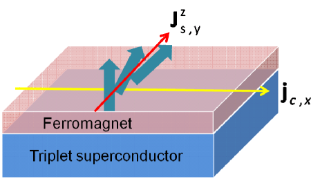
Figure 1: (Color online) Schematic of the model. Pumped charge current $j_{c,x}({\bf{x}},t)$ and the pumped spin current $j_{s,y}^{z}({\bf{x}},t)\propto\nabla_{y}\dot{{\bf{S}}}^{z}({\bf{x}},t)$ for helical $p$-wave superconductivity (Eq.(18)).

We consider a ferromagnet/triplet superconductor junction where the magnetization of the ferromagnet is inhomogeneous and dynamical as shown in Fig. 1. The Hamiltonian of the superconductor and the ferromagnet are given by $H_{S}=H_{0}+H_{\Delta}$ and $H_{F}=H_{0}+H_{ex}$, respectively. The $H_{0}$, $H_{\Delta}$ and $H_{ex}$ represent the kinetic energy, the superconducting order, and the exchange interaction between the conducting electron and the localized spins, respectively:

$$H_{0}=\sum\limits_{\bf{k}}{\phi_{\bf{k}}^{\dagger}\xi{\sigma_{0}\otimes}\tau_{3}\phi_{\bf{k}}},$$ (1)

$$H_{\Delta}=\sum\limits_{\bf{k}}{\phi_{\bf{k}}^{\dagger}\left[{({\bf{d}}_{1}\cdot{\bm{\sigma}})\otimes\tau_{1}+({\bf{d}}_{2}\cdot{\bm{\sigma}})\otimes\tau_{2}}\right]\phi_{\bf{k}}},$$ (2)

$$H_{ex}=-J\sum\limits_{{\bf{k}},{\bf{q}}}{(\phi_{{\bf{k}}-{\bf{q}}}^{\dagger}{\bm{\sigma}}\otimes\tau_{0}\phi_{\bf{k}})\cdot{\bf{S}}_{\bf{q}}}(t)$$ (3)

with $\phi_{\bf{k}}^{\dagger}=(c_{{\bf{k}}\uparrow}^{\dagger},c_{{\bf{k}}\downarrow}^{\dagger},ic_{-{\bf{k}}\downarrow},-ic_{-{\bf{k}}\uparrow})$ and $\xi=\frac{{\hbar^{2}k^{2}}}{{2m}}-\varepsilon_{F}$. Here, $\sigma$ and $\tau$ are Pauli matrices in spin and Nambu spaces, respectively. Also, $\varepsilon_{F}$, ${\bf{d}}_{j}(j=1,2)$, $J$, and $\bf{S}$ are the Fermi energy, the $\bf{d}$-vector of triplet pairing, the exchange coupling, and the localized spins, respectively. The localized spins depend on space and time, but we consider only slowly varying case. The dynamics of spins can be driven by applying magnetic field. We take into account $H_{ex}$ as a first order perturbation. Note that we adopt the basis in Ref.Ivanov such that singlet pairing is proportional to the unit matrix in spin space. With the above Hamiltonians, the charge ($j_{c,i}$) and spin current ($j_{s,i}^{\alpha}$) operators in $i$-direction read

$$j_{c,i}=-\frac{{e\hbar}}{m}k_{i}\sigma_{0}\otimes\tau_{0},\quad j_{s,i}^{\alpha}=\frac{{\hbar^{2}}}{{2m}}k_{i}\sigma_{\alpha}\otimes\tau_{3}$$ (4)

where $\alpha$ is the polarization direction of spin.

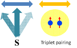
Figure 2: (Color online) Mechanism of the charge pumping. The dynamics of the localized spins is transferred to the triplet Cooper pairing via the exchange coupling. The charge pumping occurs by the dynamics of the Cooper pair with charge $-2e$.

First, let us explain physical mechanism of the charge pumping intuitively. The charge pumping occurs in the ferromagnet by the motion of proximity induced Cooper pairs as follows. In the ferromagnet, through the exchange coupling, Eq.(3), the dynamics of the localized spins is transferred to the electron’s spin. Since Cooper pair is formed by two electrons, the triplet vector also acquires dynamics (triplet vector is defined in Eq.(5)). The dynamics of the triplet vector is converted into motion of the Cooper pair via the momentum dependence of the triplet vector. Then, charge pumping occurs by the vibration of the Cooper pair with charge $-2e$ as depicted in Fig. 2. This picture is supported by the analytical expression of the pumped charge current (Eq.(15)).

Now, let us calculate the charge current and give the analytical expression. We consider the unperturbed advanced Green’s functions in the ferromagnet of the form

$$g_{{\bf{k}},\omega}^{a}=g_{0,{\bf{k}},\omega}^{a}\sigma_{0}\otimes\tau_{0}+g_{3,{\bf{k}},\omega}^{a}\sigma_{0}\otimes\tau_{3}$$

$$+({\bf{f}}_{1,{\bf{k}},\omega}^{a}\cdot{\bm{\sigma}})\otimes\tau_{1}+({\bf{f}}_{2,{\bf{k}},\omega}^{a}\cdot{\bm{\sigma}})\otimes\tau_{2}$$ (5)

where $g_{0,{\bf{k}},\omega}^{a}$ and $g_{3,{\bf{k}},\omega}^{a}$ are normal Green’s functions while ${\bf{f}}_{1,{\bf{k}},\omega}^{a}$ and ${\bf{f}}_{2,{\bf{k}},\omega}^{a}$ are 3D vector characterizing anomalous Green’s function. comment1 The charge current can be represented as Haug

$$j_{c,i}({\bf{x}},t)=\frac{{i\hbar^{2}e}}{{mV}}\sum\limits_{{\bf{k}},{\bf{q}}}{e^{-i{\bf{q}}\cdot{\bf{x}}}{\rm{Tr}}k_{i}G_{{\bf{k}}-{\bf{q}}/2,{\bf{k}}+{\bf{q}}/2}^{<}(t,t)}$$ (6)

where $V$ is the total volume and ${\rm{Tr}}$ is taken over spin and Nambu spaces. $G_{{\bf{k}}-{\bf{q}}/2,{\bf{k}}+{\bf{q}}/2}^{<}(t,t)$ is the lesser Green’s function of the total Hamiltonian. Performing perturbation with respect to $H_{ex}$, we expand the lesser component using the advanced Green’s functions by the Langreth theorem.Haug Noting that $g_{{\bf{k}},\omega}^{<}=f_{\omega}\left[{g_{{\bf{k}},\omega}^{a}-(g_{{\bf{k}},\omega}^{a})^{\dagger}}\right]$ with the lesser Green’s function $g_{{\bf{k}},\omega}^{<}$ and the Fermi distribution function $f_{\omega}$, we can compute the charge current. The first order expansion with respect to $J$ is thus given by

$$j_{c,i}({\bf{x}},t)\cong-\frac{{\hbar^{2}e}}{{Vm}}J\sum\limits_{{\bf{k}},{\bf{q}},\omega,\Omega}{e^{-i{\bf{q}}\cdot{\bf{x}}+i\Omega t}{\rm{Tr}}}k_{i}\left[{g_{{\bf{k}}-{\bf{q}}/2,\omega-\Omega/2}({\bf{S}}_{{\bf{q}},\Omega}\cdot{\bm{\sigma}})\otimes\tau_{0}g_{{\bf{k}}+{\bf{q}}/2,\omega+\Omega/2}}\right]^{<}$$

$$\cong\frac{{4\hbar^{2}eJ}}{{Vm}}\nabla_{l}\dot{\bf{S}}^{\alpha}({\bf{x}},t)\sum\limits_{{\bf{k}},\omega}{f^{\prime}_{\omega}}k_{i}{\mathop{\rm Re}\nolimits}\left[{\left({\frac{\partial}{{\partial k_{l}}}{\bf{f}}_{j,{\bf{k}},\omega}^{a}\times{\bf{f}}_{j,{\bf{k}},\omega}^{r}}\right)^{\alpha}}\right]$$ (7)

where we assume that the frequency of spin dynamics $\Omega$ is sufficiently large such that the equilibrium current is negligible compared to the dynamical one, and the repeated indices $\alpha,l$ and $j$ are summed over ($\alpha,l=1,2,3,j=1,2$). Eq.(7) is the central result of this paper. From this equation, we find that coupling of the localized spins with the triplet vector chirality in momentum space

$${\frac{\partial}{{\partial k_{l}}}{\bf{f}}_{j,{\bf{k}},\omega}^{a}\times{\bf{f}}_{j,{\bf{k}},\omega}^{r}}$$ (8)

yields the pumped charge current. Therefore, in the normal state or in the absence of the triplet vector chirality, the pumped charge current vanishes.

Similarly, the spin current can be represented as

$$j_{s,i}^{\alpha}({\bf{x}},t)=-\frac{{i\hbar^{3}}}{{2mV}}$$

$$\times\sum\limits_{{\bf{k}},{\bf{q}}}{e^{-i{\bf{q}}\cdot{\bf{x}}}{\rm{Tr}}k_{i}\sigma_{\alpha}\otimes\tau_{3}G_{{\bf{k}}-{\bf{q}}/2,{\bf{k}}+{\bf{q}}/2}^{<}(t,t)}.$$ (9)

The spin current by the first order expansion with respect to $J$ can be calculated as

$$j_{s,i}^{\alpha}({\bf{x}},t)\cong\frac{{i\hbar^{3}}}{{2mV}}J\sum\limits_{{\bf{k}},{\bf{q}},\omega,\Omega}{e^{-i{\bf{q}}\cdot{\bf{x}}+i\Omega t}{\rm{Tr}}}k_{i}\sigma_{\alpha}\otimes\tau_{3}\left[{g_{{\bf{k}}-{\bf{q}}/2,\omega-\Omega/2}({\bf{S}}_{{\bf{q}},\Omega}\cdot{\bm{\sigma}})\otimes\tau_{0}g_{{\bf{k}}+{\bf{q}}/2,\omega+\Omega/2}}\right]^{<}$$

$$=\frac{{4\hbar^{3}J}}{{Vm}}\nabla_{l}{\bf{S}}^{\beta}({\bf{x}},t)\sum\limits_{{\bf{k}},\omega}{f_{\omega}}k_{i}{\mathop{\rm Im}\nolimits}\left[{\Lambda_{{\bf{k}},\omega}^{\alpha\beta,aa}}\right]$$

$$-\frac{{2\hbar^{3}J}}{{Vm}}\nabla_{l}{\dot{\bf{S}}}^{\beta}({\bf{x}},t)\sum\limits_{{\bf{k}},\omega}{f^{\prime}_{\omega}}k_{i}\left[{\delta_{\alpha\beta}\delta_{il}{\mathop{\rm Im}\nolimits}\left\{{-\frac{\partial}{{\partial k_{l}}}g_{0,{\bf{k}},\omega}^{r}g_{3,{\bf{k}},\omega}^{a}+g_{0,{\bf{k}},\omega}^{r}\frac{\partial}{{\partial k_{l}}}g_{3,{\bf{k}},\omega}^{a}}\right\}+{\mathop{\rm Re}\nolimits}\left\{{\Lambda_{{\bf{k}},\omega}^{\alpha\beta,ra}}\right\}}\right]$$ (10)

where

$$\Lambda_{{\bf{k}},\omega}^{\alpha\beta,aa}=-\left({\frac{\partial}{{\partial k_{l}}}{\bf{f}}_{1,{\bf{k}},\omega}^{a}}\right)^{\beta}\left({{\bf{f}}_{2,{\bf{k}},\omega}^{a}}\right)^{\alpha}+\left({{\bf{f}}_{1,{\bf{k}},\omega}^{a}}\right)^{\beta}\left({\frac{\partial}{{\partial k_{l}}}{\bf{f}}_{2,{\bf{k}},\omega}^{a}}\right)^{\alpha}+\delta_{\alpha\beta}\left({\frac{\partial}{{\partial k_{l}}}{\bf{f}}_{1,{\bf{k}},\omega}^{a}\cdot{\bf{f}}_{2,{\bf{k}},\omega}^{a}-{\bf{f}}_{1,{\bf{k}},\omega}^{a}\cdot\frac{\partial}{{\partial k_{l}}}{\bf{f}}_{2,{\bf{k}},\omega}^{a}}\right)$$

$$+\left({\frac{\partial}{{\partial k_{l}}}{\bf{f}}_{2,{\bf{k}},\omega}^{a}}\right)^{\beta}\left({{\bf{f}}_{1,{\bf{k}},\omega}^{a}}\right)^{\alpha}-\left({{\bf{f}}_{2,{\bf{k}},\omega}^{a}}\right)^{\beta}\left({\frac{\partial}{{\partial k_{l}}}{\bf{f}}_{1,{\bf{k}},\omega}^{a}}\right)^{\alpha}$$ (11)

and $\Lambda_{{\bf{k}},\omega}^{\alpha\beta,ra}$ is defined by $\Lambda_{{\bf{k}},\omega}^{\alpha\beta,aa}$ with replacing ${\bf{f}}_{1,{\bf{k}},\omega}^{a}$ by ${\bf{f}}_{1,{\bf{k}},\omega}^{r}$. The first term in Eq.(10) corresponds to the equilibrium spin current while the second term describes dynamical component of the spin current, namely pumped spin current. $\Lambda_{{\bf{k}},\omega}^{\alpha\beta,aa(ra)}$ becomes zero when one of ${\bf{f}}_{1,{\bf{k}},\omega}^{a(r)}$ and ${\bf{f}}_{2,{\bf{k}},\omega}^{a}$ is zero vector. Then, the equilibrium spin current vanishes while the dynamical spin current can be present. We also see from Eq.(10) that normal component of the pumped spin current (the term containing normal Green’s functions $g_{0,{\bf{k}},\omega}^{r}$ and $g_{3,{\bf{k}},\omega}^{a}$) flowing in $i$-direction with polarization direction $\alpha$ is proportional to $\nabla_{i}\dot{\bf{S}}^{\alpha}({\bf{x}},t)$:Takeuchi

$$j_{s,i}^{(n)\alpha}({\bf{x}},t)\propto\nabla_{i}\dot{{\bf S}}^{\alpha}({\bf{x}},t).$$ (12)

Hence, we can interpret the generation of charge pumping as a result of the coupling of spin current in the normal state $j_{s,l}^{(n)\alpha}({\bf{x}},t)$ with the triplet vector chirality:

$$j_{c,i}({\bf{x}},t)\propto j_{s,l}^{(n)\alpha}({\bf{x}},t)\sum\limits_{{\bf{k}},\omega}{f^{\prime}_{\omega}}k_{i}{\mathop{\rm Re}\nolimits}\left[{\left({\frac{\partial}{{\partial k_{l}}}{\bf{f}}_{j,{\bf{k}},\omega}^{a}\times{\bf{f}}_{j,{\bf{k}},\omega}^{r}}\right)^{\alpha}}\right].$$ (13)

We see that the triplet vector chirality converts the pumped spin current into charge current. Therefore, we do not rely on spin-orbit coupling to generate charge current (convert spin current into charge current) in sharp contrast to the previous worksSaitoh ; Valenzuela .

When the direction of triplet vectors are determined only by the wavevector ${\bf{k}}$, one can decompose the triplet vectors as comment2

$${\bf{f}}_{j,{\bf{k}},\omega}^{a}=f_{j,{\bf{k}},\omega}^{a}{\bf{n}}_{j,{\bf{k}}}$$ (14)

with 3D unit vectors ${\bf{n}}_{j,{\bf{k}}}(j=1,2)$. The pumped charge current can then be written as

$$j_{c,i}({\bf{x}},t)=\frac{{4\hbar^{2}eJ}}{{Vm}}\nabla_{l}\dot{\bf{S}}^{\alpha}({\bf{x}},t)$$

$$\times\sum\limits_{{\bf{k}},\omega}{f^{\prime}_{\omega}}k_{i}\left|{f_{j,{\bf{k}},\omega}^{a}}\right|^{2}\left({\frac{\partial}{{\partial k_{l}}}{\bf{n}}_{j,{\bf{k}}}\times{\bf{n}}_{j,{\bf{k}}}}\right)^{\alpha}.$$ (15)

We find that, to obtain nonzero current, $\frac{\partial}{{\partial k_{l}}}{\bf{n}}_{j,{\bf{k}}}\neq{\bf{0}}$ is necessary. This condition means that the direction of the triplet vector depends on the wavevector ${\bf{k}}$. Namely, rotating the triplet vector induces the change of ${\bf{k}}$, which indicates that dynamics of the triplet vector leads to that of the Cooper pair. Therefore, this condition confirms the intuitive picture we have presented above.

To estimate the current, we consider transparent interface between ferromagnet and triplet superconductor such that the proxmity effect is sufficiently strong and the Green’s function in the ferromagnet has the same form as that in the bulk superconductor:

$$f_{j,{\bf{k}},\omega}^{a}=\frac{{d_{j,{\bf{k}}}}}{{(\omega-i\gamma)^{2}-\xi^{2}-\Delta_{\bf{k}}^{2}}},$$ (16)

with $\Delta_{\bf{k}}^{2}=(d_{1,{\bf{k}}})^{2}+(d_{2,{\bf{k}}})^{2}$ where $\gamma$ is the impurity scattering rate. Then, the charge current can be estimated as

$$j_{c,i}({\bf{x}},t)\cong-\frac{{\hbar^{2}e\nu J}}{{Vm}}\nabla_{l}\dot{\bf{S}}^{\alpha}({\bf{x}},t)$$

$$\times\left\langle{\frac{{k_{i}}{(d_{j,{\bf{k}}})^{2}}}{{(\gamma^{2}+\Delta_{\bf{k}}^{2})^{3/2}}}\left({\frac{\partial}{{\partial k_{l}}}{\bf{n}}_{j,{\bf{k}}}\times{\bf{n}}_{j,{\bf{k}}}}\right)^{\alpha}}\right\rangle_{FS}$$ (17)

at zero temperature where $\nu$ is the density of states at the Fermi level and $\left\langle...\right\rangle_{FS}$ means the average over the Fermi surface. As an example, let us consider helical $p$-wave superconductivity as $d_{1,{\bf{k}}}=\Delta_{0},{\bf{n}}_{1,{\bf{k}}}=1/\left|{\bf{k}}\right|(k_{y},-k_{x},0),d_{2,{\bf{k}}}=0,$ and ${\bf{n}}_{2,{\bf{k}}}={\bf{0}}$ which would be realized in non-centrosymmetric superconductor. Frigeri Then, assuming cylindrical Fermi surface, we have the pumped current flowing in $x$-direction of the form

$$j_{c,x}({\bf{x}},t)=\frac{{\hbar^{2}e\nu J}}{{2mV\Delta_{0}}}\nabla_{y}\dot{\bf{S}}^{z}({\bf{x}},t)$$ (18)

in the limit of $\gamma\to 0$. We see that the pumped charge current flows perpendicularly to the pumped spin current (note $j_{s,y}^{z}({\bf{x}},t)\propto\nabla_{y}{\dot{\bf{S}}}^{z}({\bf{x}},t)$) as illustrated in Fig. 1. As an example of the ferromagnet, we consider conical ferromagnet characterized by ${\bf{S}}({\bf{x}},t)=S(a,\cos({\bf{q}}\cdot{\bf{x}}-\Omega t),\sin({\bf{q}}\cdot{\bf{x}}-\Omega t))$ where ${\bf{q}}$ is a 3D vector which determines the spin structure, and $a$ and $\Omega$ are real constants. The charge current flowing in $x$-direction then becomes

$$j_{c,x}({\bf{x}},t)=\frac{{\hbar^{2}e\nu J}}{{2mV\Delta_{0}}}S\Omega q_{y}\sin({\bf{q}}\cdot{\bf{x}}-\Omega t).$$ (19)

Now, let us comment on the relevance of our results to SU(2) gauge field. It has been shown that the charge and spin currents in inhomogeneous magnetic structure with dynamical spin are associated with SU(2) gauge field. Volovik ; Tatara In analogy with the SU(2) gauge field in inhomogeneous magnetic structure with dynamical spin, we introduce the SU(2) gauge field by triplet spin structure. Then, the component of the SU(2) gauge field perpendicular to the adiabatic component ${\bf{n}}_{\bf{k}}$ readsVolovik ; Tatara

$${\bf{A}}_{j,{\bf{k}},\mu}^{\bot}=\frac{1}{2}{\bf{n}}_{j,{\bf{k}}}\times\frac{\partial}{{\partial k_{\mu}}}{\bf{n}}_{j,{\bf{k}}}.$$ (20)

Hence, we can represent the pumped charge current in terms of the SU(2) gauge field projected on U(1) as

$$j_{c,i}({\bf{x}},t)=-\frac{{8\hbar^{2}eJ}}{{Vm}}\nabla_{l}\dot{\bf{S}}^{\alpha}({\bf{x}},t)$$

$$\times\sum\limits_{{\bf{k}},\omega}{f^{\prime}_{\omega}}k_{i}\left|{f_{j,{\bf{k}},\omega}^{a}}\right|^{2}\left({{\bf{A}}_{j,{\bf{k}},l}^{\bot}}\right)^{\alpha}.$$ (21)

We see that the charge current is driven by the gauge field. However, since this current is also driven by dynamical spins, it has a dissipative nature (it is not a supercurrent). In the strong coupling limit, only the adiabatic component of the SU(2) gauge field, namely that projected on ${\bf{n}}_{\bf{k}}$, couples to the charge. Volovik In contrast, here the component perpendicular to ${\bf{n}}_{\bf{k}}$ contributes to the charge current. Tatara ; Taguchi2

In this paper, we have considered charge pumping in ferromagnet/triplet superconductor junctions. However, our results are also applicable to ferromagnetic superconductors where ferromagnetism and triplet superconductivity coexist in the bulk. If a ferromagnetic superconductor has some inhomogeneity such as domain wall structure, charge pumping would occur by applying ac magnetic field.

In summary, we have investigated charge pumping in ferromagnet/triplet superconductor junctions where the magnetization of the ferromagnet is inhomogeneous and dynamical. It has been shown that charge current is pumped due to the coupling of the localized spins with triplet vector chirality. This can be also interpreted as a result of the coupling between the pumed spin current and the triplet vector chirality. Physical mechanism of the charge pumping has been also presented.

This work was supported by Grant-in-Aid for Young Scientists (B) (No. 23740236) and the ”Topological Quantum Phenomena” (No. 23103505) Grant-in Aid for Scientific Research on Innovative Areas from the Ministry of Education, Culture, Sports, Science and Technology (MEXT) of Japan.

References

• (1) R. H. Silsbee, A. Janossy, and P. Monod, Phys. Rev. B 19, 4382 (1979).
• (2) Y. Tserkovnyak, A. Brataas, and G. E. W. Bauer, Phys. Rev. Lett. 88, 117601 (2002); Phys. Rev. B 66, 224403 (2002).
• (3) Y. Tserkovnyak, A. Brataas, G. E. W. Bauer, and B. I. Halperin, Rev. Mod. Phys. 77, 1375 (2005).
• (4) E. Saitoh, M. Ueda, H. Miyajima, and G. Tatara, Appl. Phys. Lett. 88, 182509 (2006).
• (5) S. O. Valenzuela and M. Tinkham, Nature (London) 442, 176 (2006).
• (6) M. Sigrist and K. Ueda, Rev. Mod. Phys. 63, 239 (1991).
• (7) Y. Maeno, H. Hashimoto, K. Yoshida, S. Nishizaki, T. Fujita, J. G. Bednorz, and F. Lichtenberg, Nature (London) 372, 532 (1994).
• (8) A. P. Mackenzie and Y. Maeno, Rev. Mod. Phys. 75, 657 (2003).
• (9) J. P. Brison, L. Glemot, H. Suderow, A. Huxley, S. Kambe, and J. Flouquet, Physica B 280, 165 (2000).
• (10) B. Kastening, D. K. Morr, D. Manske, and K. Bennemann, Phys. Rev. Lett. 96, 047009 (2006).
• (11) P. M. R. Brydon, B. Kastening, D. K. Morr, and D. Manske, Phys. Rev. B. 77, 104504 (2008).
• (12) A. Brataas and Y. Tserkovnyak, Phys. Rev. Lett. 93, 087201 (2004).
• (13) M. S. GrΓΈnsleth, J. Linder, J.-M. BΓΈrven, and A. SudbΓΈ, Phys. Rev. Lett. 97, 147002 (2006).
• (14) K. D. Nelson, Z. Q. Mao, Y. Maeno, and Y. Liu, Science 306, 1151 (2004).
• (15) J. D. Strand, D. J. Van Harlingen, J. B. Kycia, and W. P. Halperin, Phys. Rev. Lett. 103, 197002 (2009).
• (16) J. D. Strand, D. J. Bahr, D. J. Van Harlingen, J. P. Davis, W. J. Gannon, W. P. Halperin, Science 328, 1368 (2010).
• (17) D. A. Ivanov and Ya. V. Fominov, Phys. Rev. B 73, 214524 (2006).
• (18) Hereafter, ”$a$” and ”$r$” stand for advanced and retarded Green’s functions, respectively.
• (19) H. Haug and A.-P. Jauho, Quantum Kinetics in Transport and Optics of Semiconductors (Springer, New York, 1997).
• (20) A. Takeuchi and G. Tatara, J. Phys. Soc. Jpn. 77, 074701 (2008); A. Takeuchi, K. Hosono, and G. Tatara, Phys. Rev. B 81, 144405 (2010).
• (21) If the direction of ${\bf{f}}_{j,{\bf{k}},\omega}^{a}$ is determined by some factors independent of frequency such as spin-orbit coupling, (internal) magnetic field, magnetic order, or anisotropy of the system, it would be independent of the frequency. For bulk superconductor, ${\bf{n}}$ is a unit vector parallel to ${\bf{d}}$-vector of the superconductor.
• (22) P. A. Frigeri, D. F. Agterberg, A. Koga, and M. Sigrist, Phys. Rev. Lett. 92, 097001 (2004).
• (23) G. E. Volovik, J. Phys. C 20, L83 (1987).
• (24) G. Tatara, H. Kohno, and J. Shibata, Phys. Rep. 468, 213 (2008).
• (25) K. Taguchi and G. Tatara, Phys. Rev. B 79, 054423 (2009).