Random walks in random environments without ellipticity

Abstract

We consider random walks in random environments on $\mathbb{Z}^{d}$. Under a transitivity hypothesis that is much weaker than the customary ellipticity condition, and assuming an absolutely continuous invariant measure on the space of the environments, we prove the ergodicity of the annealed process w.r.t. the dynamics “from the point of view of the particle”. This implies in particular that the environment viewed from the particle is ergodic. As an example of application of this result, we prove a general form of the quenched Invariance Principle for walks in doubly stochastic environments with zero local drift (martingale condition).

MSC 2010: 60G50, 60K37, 37A50 (37A20, 60G42, 60F17).

1 Introduction

In this note we investigate random walks in random environments (RWREs) on $\mathbb{Z}^{d}$, i.e., $\mathbb{Z}^{d}$-valued Markov chains defined by the transition matrix $p(\omega)=(p_{xy}(\omega))_{x,y\in\mathbb{Z}^{d}}$, where $\omega$ is a random parameter ranging in a complete probability space $(\Omega,\Pi)$. (In the remainder we will refer to either $\omega$ or $p(\omega)$ as the environment.)

Although the precise nature of $\Omega$ is irrelevant, a natural choice is $\Omega=(\mathcal{S}_{K,\gamma})^{\otimes\mathbb{Z}^{d}}$, where, for $K,\gamma>0$, $\mathcal{S}_{K,\gamma}$ is the space of all probability distributions $\omega_{o}=(\omega_{oy})_{y\in\mathbb{Z}^{d}}$ on $\mathbb{Z}^{d}$, such that $\omega_{oy}\leq K|y|^{-d-\gamma}$. By tightness [B2], $\mathcal{S}_{K,\gamma}$ is compact in the weak-* topology, which can be metrized, e.g., by the total variation distance between two distributions. Hence, by Tychonoff’s Theorem and a standard argument, $\Omega$ is also compact and metrizable. (This is important in case one needs to construct suitable invariant measures.) For an element $\omega=(\omega_{x})_{x\in\mathbb{Z}^{d}}\in\Omega$, where $\omega_{x}=(\omega_{xy})_{y\in\mathbb{Z}^{d}}\in\mathcal{S}_{K,\gamma}$, $p(\omega)$ is defined by $p_{xy}(\omega):=\omega_{x,y-x}$.

$\Omega$ is acted upon by $\mathbb{Z}^{d}$ via the group of $\Pi$-automorphisms $(\tau_{z})_{z\in\mathbb{Z}^{d}}$, such that

$$p_{xy}(\tau_{z}\omega)=p_{x+z,y+z}(\omega).$$ (1.1)

(In the representation above, $\tau_{z}$ is defined as $(\tau_{z}\omega)_{x}:=\omega_{x+z}$.) Because of this, there is no loss of generality in requiring that the walk always starts at $0$. The random walk (RW) in the environment $p(\omega)$ is then be defined as the Markov chain $(X_{n})_{n\in\mathbb{N}}$ on $\mathbb{Z}^{d}$ whose law $P_{\omega}$ is uniquely determined by

$$P_{\omega}(X_{0}=0)=1;$$ (1.2)

$$P_{\omega}(X_{n+1}=y\,|\,X_{n}=x)=p_{xy}(\omega).$$ (1.3)

The complete randomness of the problem is accounted for by the annealed (or averaged) law, which is defined on $(\mathbb{Z}^{d})^{\mathbb{N}}\times\Omega$ via

$$\mathbb{P}(E\times B):=\int_{B}\Pi(d\omega)\,P_{\omega}(E),$$ (1.4)

where $E$ is a Borel set of $(\mathbb{Z}^{d})^{\mathbb{N}}$ (the latter being the space of the trajectories, where $P_{\omega}$ is defined) and $B$ is a measurable set of $\Omega$. A natural dynamics that can be defined on this process is the one induced by the map $\mathcal{F}:(\mathbb{Z}^{d})^{\mathbb{N}}\times\Omega\longrightarrow(\mathbb{Z}^{d})^{\mathbb{N}}\times\Omega$, given by

$$\mathcal{F}\left((x_{n})_{n\in\mathbb{N}}\,,\omega\right):=\left((x_{n+1})_{n\in\mathbb{N}}\,,\tau_{x_{1}}\omega\right).$$ (1.5)

As is apparent, the first component of $\mathcal{F}$ updates the trajectory of the RW to the next time, while the second component updates the environment as seen by the random walker, or particle. This dynamics may thus be called ‘the point of view of the particle’ (PVP) for the annealed process.

Another process of great importance, which is directly related to the above, is the so-called ‘environment viewed from the particle’ (EVP). It can be defined independently as the Markov chain $(\Omega_{n})_{n\in\mathbb{N}}$ on $\Omega$, with law $\mathcal{P}_{\Pi}$, such that:

$$\mathcal{P}_{\Pi}(\Omega_{0}\in B)=\Pi(B);$$ (1.6)

$$\mathcal{P}_{\Pi}(\Omega_{n+1}=\omega\,|\,\Omega_{n}=\omega^{\prime})=\sum_{y:\,\tau_{y}\omega^{\prime}=\omega}p_{0y}(\omega^{\prime}).$$ (1.7)

(The annoying notation whereby $\Omega_{n}$ denotes an element of $\Omega$ will be used only once more in this note, in the statement of (A1).)

Notational convention. Throughout the paper, the dependence of whichever quantity (e.g., $p$) on $\omega$ will not be explicitly indicated when there is no risk of confusion.

When studying the stochastic properties of a RWRE, say, proving the quenched Central Limit Theorem (CLT) (i.e., the CLT relative to $P_{\omega}$, for $\Pi$-a.a. $\omega\in\Omega$), the state-of-the-art technique requires one to face more or less three hurdles:

1. showing the existence of a steady state for the EVP that is absolutely continuous w.r.t. the original measure;

2. proving certain basic ergodic properties of the steady state;

3. controlling the error term between the random walk and an approximating martingale.

An assumption that is almost always made is the ellipticity of the environment. We state two rather general versions it may come in.

Definition 1.1

A random environment $(\Omega,\Pi)$ is called elliptic if there exists a basis $\Lambda$ of $\mathbb{Z}^{d}$ such that, for $\Pi$-a.a. $\omega\in\Omega$ and all $e\in\Lambda$, $p_{0e}>0$. It is called uniformly elliptic if there also exists $\varepsilon>0$ such that, in the same cases as before, $p_{0e}\geq\varepsilon$.

To the author’s knowledge, at least within the scope of non-ballistic RWREs, only a few results [Be, SS, BB, MP, BeD] do not assume ellipticity. In general, uniform ellipticity is required—although recent work focuses on non-uniformly elliptic systems; cf. [M, GZ, Sa] and references therein.

There are reasons to consider the ellipticity condition rather unsatisfactory; for example, uniform ellipticity is a deterministic condition in a probabilistic problem. The purpose of this note is to show that, among the three hurdles mentioned above, ellipticity might only be important for the first one. Certainly it is not needed for the second. (The third hurdle is outside the scope of this article, but the indication is that ellipticity is not particularly useful there either. See also Section 4.)

We replace ellipticity with the hypothesis that a relevant set of environments are transitive, i.e., a walker starting at the origin goes anywhere with positive probability. We call this partial transitivity. (In actuality, our hypotheses are more general than that; cf. (A3)-(A5) below.) We say that (total) transitivity holds if a.e. environment is transitive. A certain form of transitivity, together with the ergodicity of the environment w.r.t. translations, seems like a natural, somewhat minimal, assumption, if we want the particle to “test” every environment. A discussion on the merits of our hypothesis is given below.

In a general setting, we show that, if an absolutely continuous steady state is given on the space of the environments (that is, if hurdle 1 is taken care of), and if its support contains transitive environments, the steady state and the original state are equivalent measures, and the PVP process, relative to either, is ergodic (Theorem 1.3). The same is true for the EVP process (Corollary 1.4).

The simplest environments for which the above hypothesis holds are the doubly stochastic environments, for which $\Pi$ is automatically invariant in the right sense. If we further assume the RW to be a martingale (doing away with hurdle 3 as well) one gets the Invariance Principle (IP) too (Theorem 4.2).

Assumptions. The RWRE satisfies the following:

• No deterministic walks. Denote by $\delta_{xy}$ the Kronecker delta in $\mathbb{Z}^{d}$ and set

  $$\Omega_{\mathrm{d}}:=\left\{\omega\in\Omega\>\left|\>\exists y_{o}\in\mathbb{Z}^{d}\mbox{ such that }p_{0y}=\delta_{y_{o}y},\forall y\in\mathbb{Z}^{d}\right.\!\right\}.$$

  (This is the set of environments that have a deterministic jump at the origin.) We have that, $\mathbb{P}$-almost surely, $(\Omega_{n})_{n\in\mathbb{N}}\not\subset\Omega_{\mathrm{d}}$. In other words, in a.e. environment, the random walk starting at the origin is not deterministic.

• Decaying transition probabilities. There exist $K,\gamma>0$ such that, almost surely,

  $$p_{xy}\leq K|y-x|^{-d-\gamma}.$$

• Ergodicity. There is a subgroup $\Gamma\subseteq\mathbb{Z}^{d}$ such that $(\Omega,\Pi,(\tau_{z})_{z\in\Gamma})$ is ergodic. (In particular, the random environment is ergodic w.r.t. the whole group of translations.)

• Partial transitivity. Let $\Gamma$ be the same as in (A3). Define

  $$\Omega_{\mathrm{t}}:=\left\{\omega\in\Omega\>\left|\>\forall y\in\Gamma,\ \exists n=n(\omega,y)\mbox{ such that }p^{(n)}_{0y}>0\right.\!\right\},$$

  where $p^{(n)}_{0y}:=\sum_{x_{1},\ldots,x_{n-1}}p_{0x_{1}}\,p_{x_{1}x_{2}}\cdots\,p_{x_{n-1}y}$. (This is the set of transitive environments.) It must be that $\Pi(\Omega_{\mathrm{t}})>0$.

• Absolute continuity of steady state. There exists a probability measure $\Pi_{*}$ on $\Omega$, absolutely continuous w.r.t. $\Pi$, such that the EVP process $\mathcal{P}_{\Pi_{*}}$, defined as in (1.6)-(1.7), is stationary. Furthermore, $\Pi(\mathrm{supp}_{\Pi}\,\Pi_{*}\cap\Omega_{\mathrm{t}})>0$; equivalently, $\Pi_{*}(\Omega_{\mathrm{t}})>0$.

Notice that there is a trade-off between (A3) and (A4): if $\Gamma$ gets smaller, thus making (A3) stronger, then (A4) becomes easier to verify, and viceversa. In particular, for an i.i.d. environment (namely, the stochastic vectors $p_{x}=(p_{xy})_{y\in\mathbb{Z}^{d}}$ are i.i.d. in $x$), one only need verify partial transitivity w.r.t. $\Gamma=\mathbb{Z}y_{o}$, for some $y_{o}\in\mathbb{Z}^{d}$. In any event, $\Gamma=\mathbb{Z}^{d}$ is a reasonable choice for many applications. For further observations on (A4), see Remark 3.6.

Remark 1.2

In (A5), the hypothesis of absolute continuity could be replaced by the (slightly) weaker condition that the steady state $\Pi_{*}$ is non-singular w.r.t. $\Pi$. The two conditions are actually equivalent in our case. In fact, it can be seen (cf. Section 2) that the evolution of $\Pi$ in the EVP process is absolutely continuous w.r.t. $\Pi$, which implies that, if $\Pi_{*}$ decomposes into an absolutely continuous measure and a singular measure, both of them are invariant for the process.

Results. These are our main results:

Theorem 1.3

Under assumptions (A1)-(A5),

• the measures $\Pi$ and $\Pi_{*}$ are equivalent (i.e., mutually absolutely continuous);

• if $\mathbb{P}_{*}$ is the annealed law relative to $\Pi_{*}$ (i.e., the measure defined by (1.4) with $\Pi_{*}$ in lieu of $\Pi$), then $\mathbb{P}_{*}$ is stationary and ergodic for the dynamics induced by $\mathcal{F}$ on the annealed process;

• $\Pi(\Omega_{\mathrm{t}})=1$.

Corollary 1.4

The EVP with initial state $\Pi_{*}$ is ergodic.

Another easy corollary of Theorem 1.3 concerns the ballisticity of the RW. In order to state it, we introduce the mean displacement (or local drift) at the origin, for the environment $\omega$. This is the function $\mathcal{D}:\Omega\longrightarrow\mathbb{Z}^{d}$ given by

$$\mathcal{D}(\omega):=\sum_{y\in\mathbb{Z}^{d}}p_{0y}(\omega)\,y,$$ (1.8)

which is surely well-defined if $\gamma$ in (A2) is bigger than 1.

Corollary 1.5

If the local drift (1.8) is well-defined in $L^{1}(\Omega,\Pi)$, then, for $\Pi$-a.e. environment $\omega$,

$$\lim_{n\to\infty}\frac{X_{n}}{n}=\int_{\Omega}\Pi_{*}(d\omega^{\prime})\,\mathcal{D}(\omega^{\prime}),$$

$P_{\omega}$-almost surely.

Discussion. Theorem 1.3 is a “soft result”, in the sense that it is very general and not very deep. Certainly it is not surprising, as analogous statements were already known in several specific cases, e.g., [L1, L2, BK, KO, SS, BB, MP, M, BaD, GZ, Sa, BeD]. But this is actually the point of this note: to show that the ergodicity of the PVP is a general result that need not be proved every time, provided one has an absolutely continuous invariant measure for the EVP, and transitivity somewhere in its support. In other words, hurdle 2 is not a hurdle.

It might be worthwhile to point out that Theorem 1.3 is not obvious from Koslov’s 1985 paper [K] (at least not to this author).

Recently, Berger and Deuschel [BeD] proved the quenched IP for RWs in i.i.d., nearest-neighbor, balanced environments (in the sense of [L1, L2]), under the assumption of genuine $d$-dimensionality (g.$d$-d.). The latter means that, for every $e\in\mathbb{Z}^{d}$ with $|e|=1$, $\Pi(p_{0e}(\omega)>0)>0$. Clearly, this is weaker than our transitivity; strictly weaker, in fact, as we discuss below.

In light of this result, one might think that g.$d$-d. is a better condition than transitivity and would produce a more general version of Theorem 1.3. We claim that this is not really the case. First we argue that, within the scope of [BeD], g.$d$-d. is similar in spirit to transitivity. Then, by way of a counterexample, we show that Theorem 1.3 could not hold in its generality if transitivity were replaced by g.$d$-d.

Under the assumptions of [BeD], it is easy to find examples where, almost surely, there are sites that the particle cannot visit (see, e.g., Fig. 3 of [BeD]). It turns out, however, that a.e. environment has a sink, that is, a subset of $\mathbb{Z}^{d}$ that each trajectory enters, in finite time, and never leaves. The sink is unique, unbounded, and transitive. The environments seen from the sink make up the support of the steady state $\Pi_{*}$ (whose $\Pi$-measure may be less than 1) and its ergodic properties depend on the fact that it is transitive.

As for the other point—disproving Theorem 1.3 under the hypothesis of g.$d$-d.—we have just shown that assertion (a) may not be true. This is no big trouble, as long as one proves that, after a controlled time, the EVP falls in the support of $\Pi_{*}$ (this is the case in [BeD]). But there are examples in which assertion (b) fails as well.

For instance, let $(\xi_{j})_{j\in\mathbb{Z}}$ be i.i.d. random variables taking the values (labels) A or B, both with positive probability. Each realization of this Bernoulli chain defines an environment on $\mathbb{Z}^{2}$ by assigning to the site $x=(j,k)$ the same label as the variable $\xi_{j}$. Thus, the random environment is constant for the vertical translations and ergodic for the horizontal ones, whose subgroup we denote $\Gamma$; cf. (A3). It is then ergodic. Prescribe that, when the particle visits a site of type A, it has probability 1/2 to make the next move to the left and probability 1/2 to make it to the right; when it visits a site of type B, the rule is analogous, but for up/down moves. Clearly, g.$d$-d. holds but transitivity (almost) never does, even for $\Gamma$; cf. (A4). The associated PVP and EVP processes have quite trivial dynamics: in particular, the elementary steady states for the EVP are atoms, corresponding to environments whose entire vertical axis is labeled B. This shows that an absolutely continuous steady state $\Pi_{*}$ cannot make those processes ergodic.

Remark 1.6

The fact that the above environment is balanced with nearest-neighbor jumps, and g.$d$-d. holds, proves that a strong mixing property is essential for the result of [BeD].

Our proofs are based on a convenient representation of the RWRE as a probability-preserving dynamical system which, roughly speaking, is a “measured family” of one-dimensional Markov maps. Each map embodies the dynamics of one random jump, and thus contains only local information. We will see that this dynamical system is isomorphic to the annealed process. In any case, Section 2 should convince the reader that it is natural to call this object ‘the dynamical system for the point of view of the particle’; in short, PVP dynamical system.

The exposition is organized as follows: In Section 2 we introduce the dynamical system and find a suitable invariant measure for it. In Section 3 we prove its ergodicity, which is equivalent to Theorem 1.3 and implies its corollaries. In Section 4 we consider the example of the doubly stochastic RWs, proving an improved version of the quenched IP for doubly stochastic martingales.

Acknowledgments. I am grateful to Alessandra Bianchi, Firas Rassoul-Agha, Frank den Hollander, Luc Rey-Bellet, Vladas Sidoravicius and Stefano Olla for useful discussions. I also thank an anonymous referee for a careful reading of the early versions of the manuscript. This work was partially supported by the FIRB-“Futuro in Ricerca” Project RBFR08UH60 (MIUR, Italy).

2 The PVP dynamical system

Let us fix an enumeration $(d_{i})_{i\in\mathbb{Z}_{+}}$ of $\mathbb{Z}^{d}$. For $\omega\in\Omega$ and $i\in\mathbb{Z}_{+}$, we define

$$q_{i}(\omega):=p_{0d_{i}}(\omega)\\$$ (2.1)

Certainly, $\sum_{i}q_{i}(\omega)=1$. We then set $a_{0}(\omega):=0$ and, recursively on $i$,

$$a_{i}(\omega):=a_{i-1}(\omega)+q_{i}(\omega)$$ (2.2)

$$I_{i}(\omega):=[a_{i-1}(\omega)\,,\,a_{i}(\omega)).$$ (2.3)

Clearly, $\{I_{i}(\omega)\}_{i\in\mathbb{Z}_{+}}$ is a partition of $I:=[0,1)$. For $(s,\omega)\in I\times\Omega$, denote by $i(s,\omega)$ the unique $i$ such that $s\in I_{i}(\omega)$. We define the function $\phi:I\times\Omega\longrightarrow I$ via

$$\phi(s,\omega):=\frac{s-a_{i(s,\omega)-1}(\omega)}{q_{i(s,\omega)}(\omega)}.$$ (2.4)

(The definition above is well-posed because, if $i$ is such that $q_{i}(\omega)=0$, there is no $s$ such that $i(s,\omega)=i$.) By construction, $\phi(\cdot,\omega)$ is the perfect Markov map $I\longrightarrow I$ relative to the partition $\{I_{i}(\omega)\}$, namely, each branch of this map is affine and its image is $I$. Finally, we denote $D(s,\omega):=d_{i(s,\omega)}$.

The main technical tool of this paper is the map $T:\mathcal{M}\longrightarrow\mathcal{M}$, defined on $\mathcal{M}:=I\times\Omega$ by

$$T(s,\omega):=\left(\phi(s,\omega),\tau_{D(s,\omega)}\omega\right).$$ (2.5)

We endow $\mathcal{M}$ with either the probability measure $\mu:=m\otimes\Pi$ or $\mu_{*}:=m\otimes\Pi_{*}$, where $m$ is the Lebesgue measure on $I$.

What this dynamical system has to do with our RWRE is presently explained. Let us recall the notational convention whereby the dependence on $\omega$ is not always indicated. Fix $\omega\in\Omega$ and consider a random $s\in I$ w.r.t. $m$. We have that $D(s,\omega)=d_{i}$ if and only if $s\in I_{i}$, and this occurs with probability $m(I_{i})=q_{i}$. In terms of our RW, this is exactly the probability that a particle placed in the origin of $\mathbb{Z}^{d}$, endowed with the environment $p(\omega)$, jumps by a quantity $d_{i}$. Then, back to the dynamical system, condition the measure $m$ to $I_{i}$. Calling $(s_{1},\omega_{1}):=T(s,\omega)$, we see that, upon conditioning, $s_{1}$ ranges in $I$ with law $m$. Therefore, in a sense, the variable $s$ (which we may call the internal variable) has “refreshed” itself. Furthermore, $\omega_{1}=\tau_{D(s,\omega)}\omega=\tau_{d_{i}}\omega$ is the translation of $\omega$ in the opposite direction to $d_{i}$; cf. (1.1). Hence we can imagine that we have reset the system to a new initial condition $(s_{1},\omega_{1})$, corresponding to the particle sitting in $0\in\mathbb{Z}^{d}$ and subject to the environment $p(\omega_{1})$. Applying the same reasoning to $(s_{2},\omega_{2}):=T(s_{1},\omega_{1})$, and so on, shows that we are following the motion “from the point of view of the particle”. We thus call the above the ‘PVP dynamical system’.

In any case, it should be clear that the stochastic process $(X_{n})_{n\in\mathbb{N}}$, with $X_{0}\equiv 0$ and, for $n\geq 1$,

$$X_{n}(s,\omega):=\sum_{k=0}^{n-1}D\circ T^{k}(s,\omega).$$ (2.6)

is precisely the RW in the environment $p(\omega)$, provided that $\omega$ is regarded as a fixed parameter. To emphasize this point, we occasionally write $X_{n,\omega}(s):=X_{n}(s,\omega)$. $(X_{n,\omega})$ is called the ‘quenched trajectory’, and it is a Markov chain. If both $s$ and $\omega$ are considered random, w.r.t. $\mu$, then (2.6) defines the ‘annealed trajectory’. This is not a Markov chain and, by the definition of $\mu$ and (1.4), it is none other than the RWRE of Section 1 with law $\mathbb{P}$. For a formal relation between the annealed process and the PVP dynamical system see Proposition 3.2.

Proposition 2.1

The measure $\mu_{*}$ is preserved by $T$.

We need the following lemma:

Lemma 2.2

For every measurable set $B\subseteq\Omega$,

$$\Pi_{*}(B)=\sum_{i\in\mathbb{Z}_{+}}\int_{\tau_{-d_{i}(B)}}\Pi_{*}(d\omega^{\prime})\,q_{i}(\omega^{\prime}).$$

Proof of Lemma 2.2. Via (2.1) and (A2), we observe that the series

$$\sum_{i\in\mathbb{Z}_{+}}q_{i}(\omega^{\prime})=\sum_{x\in\mathbb{Z}^{d}}p_{0x}(\omega^{\prime}),$$ (2.7)

is uniformly bounded in $\omega^{\prime}$. Thus, as we will do more than once presently, it is correct to interchange the above summation with an integration over $\Omega$, if it is relative to a probability measure.

Using again (2.1), the transition kernel of the EVP process (1.7) can be written as

$$\mathcal{K}(\omega^{\prime},\,\cdot\,)=\sum_{i\in\mathbb{Z}_{+}}q_{i}(\omega^{\prime})\,\delta_{\tau_{d_{i}}\omega^{\prime}},$$ (2.8)

where the Dirac delta on the r.h.s. is thought of as a measure. In other words, for a measurable set $B$,

$$\mathcal{K}(\omega^{\prime},B)=\int_{\Omega}\mathcal{K}(\omega^{\prime},d\omega)\,1_{B}(\omega)=\sum_{i\in\mathbb{Z}_{+}}q_{i}(\omega^{\prime})\,1_{\tau_{-d_{i}(B)}}(\omega^{\prime}).$$ (2.9)

Thus, the hypothesis on $\Pi_{*}$ from (A5), namely,

$$\Pi_{*}(B)=\int_{\Omega}\Pi_{*}(d\omega^{\prime})\,\mathcal{K}(\omega^{\prime},B),$$ (2.10)

reads precisely as in the statement of the lemma. Q.E.D.

Proof of Proposition 2.1. It is enough to prove that $\mu_{*}(T^{-1}A)=\mu_{*}(A)$ for all sets of the type $A=[b,c)\times B$, where $B$ is a measurable set of $\Omega$.

By direct inspection of the map (2.5), we can write $T^{-1}A=\bigcup_{i\in\mathbb{Z}_{+}}A^{\prime}_{i}$, where

$$A^{\prime}_{i}:=\left\{(s^{\prime},\omega^{\prime})\>\left|\>\omega^{\prime}\in\tau_{-d_{i}}(B),\,s^{\prime}\in[a_{i}(\omega^{\prime})+q_{i}(\omega^{\prime})b\,,\,a_{i}(\omega^{\prime})+q_{i}(\omega^{\prime})c)\right.\!\right\};$$ (2.11)

cf. (2.2), (2.4). Thus,

$$\mu_{*}(A^{\prime}_{i})=\int_{\tau_{-d_{i}}(B)}\Pi_{*}(d\omega^{\prime})\,q_{i}(\omega^{\prime})(c-b).$$ (2.12)

The sets $A^{\prime}_{i}$ are pairwise disjoint because, by construction, they belong to different level sets of the function $D$. Therefore, by Lemma 2.2,

$$\mu_{*}(T^{-1}A)=(c-b)\sum_{i\in\mathbb{Z}_{+}}\int_{\tau_{-d_{i}}(B)}\Pi_{*}(d\omega^{\prime})\,q_{i}(\omega^{\prime})=(c-b)\,\Pi_{*}(B)=\mu_{*}(A),$$ (2.13)

which is what we wanted to prove. Q.E.D.

Let us introduce a convenient notation that will be used throughout the paper: For $(s,\omega)\in\mathcal{M}$ and $k\in\mathbb{N}$, denote

$$(s_{k},\omega_{k}):=T^{k}(s,\omega).$$ (2.14)

Proposition 2.3

The measures $\mu_{*}$ and $\mu$ are equivalent or, which is the same, the measures $\Pi_{*}$ and $\Pi$ are equivalent.

Proof. Denote $\Omega_{*}:=\mathrm{supp}_{\Pi}\,\Pi_{*}$, $\Omega_{\mathrm{*t}}:=\Omega_{*}\cap\Omega_{\mathrm{t}}$, and $\Omega_{*}^{c}:=\Omega\setminus\Omega_{*}$. By (A5), $\Pi(\Omega_{\mathrm{*t}})>0$ and $\Pi(\Omega_{*}^{c})<1$. Suppose, by way of contradiction, that $\Pi(\Omega_{*}^{c})>0$ as well.

By (A3), for $\Pi$-a.e. $\omega\in\Omega_{\mathrm{*t}}$, there exists $y_{\omega}\in\Gamma$ such that

$$\tau_{y_{\omega}}\omega\in\Omega_{*}^{c}.$$ (2.15)

To each such $\omega$ (excluding at most a $\Pi$-null set) we apply (A4) and its interpretation in terms of the PVP dynamical system: there exists a positive integer $n=n(\omega,y_{\omega})$ such that

$$J_{\omega}:=\left\{s\in I\>\left|\>X_{n}(s,\omega)=y_{\omega}\right.\!\right\}$$ (2.16)

has measure $p_{0y_{\omega}}^{(n)}>0$. By definition, $\forall s\in J_{\omega}$,

$$T^{n}(s,\omega) = (s_{n},\tau_{D(s_{n-1},\omega_{n-1})}\circ\cdots\circ\tau_{D(s,\omega)}\,\omega)$$ (2.17)

$$= (s_{n},\tau_{X_{n}(s,\omega)}\,\omega)$$

$$= (s_{n},\tau_{y_{\omega}}\omega)\in I\times\Omega_{*}^{c},$$

having used (2.14), (2.6), (2.16) and finally (2.15). If we define

$$A:=\bigcup_{\omega\in\Omega_{\mathrm{*t}}}J_{\omega}\times\{\omega\},$$ (2.18)

we have $\mu(A)>0$ and, via (2.17),

$$A\subset\bigcup_{n\geq 1}T^{-n}(I\times\Omega_{*}^{c}).$$ (2.19)

The definition of $\Omega_{*}^{c}$ implies that $\mu_{*}(I\times\Omega_{*}^{c})=0$, hence, since $\mu_{*}$ is $T$-invariant, $\mu_{*}(A)=0$. Finally, since $\mu$ and $\mu_{*}$ are equivalent on $I\times\Omega_{*}\supset A$, $\mu(A)=0$, which contradicts a previous statement. Q.E.D.

For a graphic representation of the above proof, see Fig. 1 and its caption.

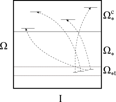
Figure 1: Representation of $\mathcal{M}=I\times\Omega$ as a square for the proof of Proposition 2.3. By the ergodicity of the random environment and partial transitivity, in a.e. horizontal segment (later denoted by horizontal fiber) of $\Omega_{\mathrm{*t}}\subseteq\Omega_{\mathrm{t}}$, one can find a subsegment (denoted by $J_{\omega}\times\{\omega\}$ in the proof) that the dynamics takes “everywhere in $\mathcal{M}$” that has been established. In this way, one carries a positive $\mu$-measure into $I\times\Omega_{*}^{c}$, the complement of supp$\,\mu_{*}$, which therefore cannot be $\mu$-null.

3 Ergodicity

In this section we will prove the ergodicity of $(\mathcal{M},\mu_{*},T)$. For this, we need to introduce some more notation and establish a few lemmas.

Given a positive integer $n$ and a multi-index $\mathbf{i}:=(i_{0},i_{1},...,i_{n-1})\in\mathbb{Z}_{+}^{n}$, we set

$$I_{\mathbf{i}}(\omega):=\left\{s\in I\>\left|\>D\circ T^{k}(s,\omega)=d_{i_{k}},\>\forall k=0,\ldots,n-1\right.\!\right\}.$$ (3.1)

For $n=1$ this reduces to definition (2.3). It is easy to ascertain that $\{I_{\mathbf{i}}\}_{\mathbf{i}\in\mathbb{Z}_{+}^{n}}$ is a partition of $I$ into countably many (possibly empty) right-open intervals, each of which corresponds to one of the realizations of the RW $(X_{k,\omega})_{k=0}^{n}$ (relative to the environment $\omega$) in such a way that $m(I_{\mathbf{i}})$ is the probability of the corresponding realization. In analogy with the previous notation, we denote by $\mathbf{i}_{n}(s,\omega)$ the index of the element of the partition which contains $s$.

Furthermore, let us call horizontal fiber of $\mathcal{M}$ any segment of the type $I_{\omega}:=I\times\{\omega\}$, and indicate with $m_{\omega}$ the Lebesgue measure on it. Finally, we denote by $I_{\omega,\mathbf{i}}$ the subset of $I_{\omega}$ corresponding to $I_{\mathbf{i}}(\omega)$ via the natural isomorphism $I\cong I_{\omega}$.

Lemma 3.1

For a.a. $(s,\omega)\in\mathcal{M}$, $m(I_{\mathbf{i}_{n}(s,\omega)})$ vanishes exponentially fast, as $n\to\infty$.

Proof. Set

$$f(s,\omega):=\log q_{i(s,\omega)}^{-1}(\omega)=-\log m(I_{i(s,\omega)}(\omega)).$$ (3.2)

Clearly $f(s,\omega)\geq 0$, with $f(s,\omega)=0$ if and only if $\{I_{i}(\omega)\}$ is the trivial partition of $I$, if and only if $\omega\in\Omega_{\mathrm{d}}$; cf. (A1). The Birkhoff average of $f$,

$$f^{+}(s,\omega):=\lim_{n\to\infty}\,\frac{1}{n}\,\sum_{k=0}^{n-1}\,f(s_{k},\omega_{k}),$$ (3.3)

is non-negative as well. Set $A:=\left\{(s,\omega)\>\left|\>f^{+}(s,\omega)=0\right.\!\right\}$. As a level set of an invariant function, $A$ is invariant mod $\mu_{*}$. We claim that $\mu_{*}(A)=0$. If not, we can apply one of the assertions of Birkhoff’s Theorem to the measure-preserving dynamical system $(A,\mu_{*},T_{|A})$ and conclude that $\int_{A}d\mu_{*}\,f=\int_{A}d\mu_{*}\,f^{+}=0$. Therefore, $f(s,\omega)=0$, for a.a. $(s,\omega)\in A$. In other words, $A\subseteq I\times\Omega_{\mathrm{d}}$ mod $\mu_{*}$. Since $A$ is invariant, the orbit of a.e. point in $A$ is contained in $I\times\Omega_{\mathrm{d}}$, implying that $(\omega_{n})_{n\in\mathbb{N}}\subset\Omega_{\mathrm{d}}$ for a positive measure of initial conditions—in contradiction with (A1).

So $f^{+}>0$ almost everywhere. On the other hand, from earlier considerations, it is easy to verify that, for $n\geq 1$,

$$m\left(I_{\mathbf{i}_{n}(s,\omega)}(\omega)\right)=\prod_{k=0}^{n-1}q_{i(s_{k},\omega_{k})}(\omega_{k})=\exp\left(-\sum_{k=0}^{n-1}f(s_{k},\omega_{k})\right).$$ (3.4)

Due to the almost sure positivity of (3.3), the exponent in the rightmost term above is asymptotically linear in $n$, for a.a. $(s,\omega)$, which yields the assertion. Q.E.D.

Proposition 3.2

As dynamical systems on probability spaces, $(\mathcal{M},\mu,T)$ is isomorphic to $((\mathbb{Z}^{d})^{\mathbb{N}}\times\Omega,\mathbb{P},\mathcal{F})$, and $(\mathcal{M},\mu_{*},T)$ is isomorphic to $((\mathbb{Z}^{d})^{\mathbb{N}}\times\Omega,\mathbb{P}_{*},\mathcal{F})$.

Proof. We hope the reader was already convinced in Section 2 that the PVP dynamical system describes exactly the annealed process with the PVP dynamics. On the other hand, Lemma 3.1 provides the ingredients for a formal proof, which we just sketch here.

For both pairs of systems, a natural isomorphism $\Phi:\mathcal{M}\longrightarrow(\mathbb{Z}^{d})^{\mathbb{N}}\times\Omega$ is given by

$$\Phi(s,\omega):=\left((X_{n}(s,\omega))_{n\in\mathbb{N}}\,,\omega\right);$$ (3.5)

cf. (2.6). One sees that $\Phi$ is almost-everywhere bijective because of the following: By Lemma 3.1, a.e. $(s,\omega)\in\mathcal{M}$ is the unique intersection point of the nested sequence of right-open intervals $(I_{\omega,\mathbf{i}_{n}(s,\omega)})_{n\in\mathbb{N}}$, i.e., is uniquely determined by the sequence $(\mathbf{i}_{n}(s,\omega))$, equivalently, by the realization $(X_{n}(s,\omega))$ of the RW. Viceversa, for an environment $\omega$, every realization of the walk determines a nested sequence of intervals which, except for a null set of realizations, gives a point $(s,\omega)\in I_{\omega}$. (Since the intervals are right-open, this correspondence is ill-defined at the endpoints of all such intervals. But this amounts to a null set of points in $I_{\omega}$ and a null set of realizations in $(\mathbb{Z}^{d})^{\mathbb{N}}$.)

Finally, it is clear by the considerations of Section 2 that $\mu=\mathbb{P}\circ\Phi$, $\mu_{*}=\mathbb{P}_{*}\circ\Phi$ and $T=\Phi^{-1}\circ\mathcal{F}\circ\Phi$. Q.E.D.

Lemma 3.3

The ergodic components of $(\mathcal{M},\mu_{*},T)$ contain whole horizontal fibers, that is, every invariant set is of the form $I\times B$, mod $\mu_{*}$ (equivalently, mod $\mu$), where $B$ is a measurable subset of $\Omega$.

Proof. The idea of the proof is that, since $T$ maps subintervals of horizontal fibers onto whole horizontal fibers (the “perfect Markov” property of Section 2), its repeated application stretches any set horizontally to the full length of the horizontal fibers. An invariant set must thus contain full fibers. Now for a formal proof.

Suppose the assertion of Lemma 3.3 is false. There exists an invariant set $A$ whose intersection with many horizontal fibers is neither the full fiber nor empty, mod $m_{\omega}$. That is, for some $\varepsilon>0$, the $\Pi_{*}$-measure of

$$B_{\varepsilon}:=\left\{\omega\in\Omega\>\left|\>m_{\omega}(A\cap I_{\omega})\in[\varepsilon,1-\varepsilon]\right.\!\right\}$$ (3.6)

is positive. By the Poincaré Recurrence Theorem and the Lebesgue Density Theorem it is possible to pick $(s,\omega)\in A\cap(I\times B_{\varepsilon})$ that is recurrent to $I\times B_{\varepsilon}$ and such that $(s,\omega)$ is a density point of $A\cap I_{\omega}$, within $I_{\omega}$, relative to $m_{\omega}$. We claim that there exist a sufficiently large $n$ and a multi-index $\mathbf{i}\in\mathbb{Z}_{+}^{n}$ for which

$$m_{\omega}(A\cap I_{\omega,\mathbf{i}})>(1-\varepsilon)\,m_{\omega}(I_{\omega,\mathbf{i}})$$ (3.7)

and

$$T^{n}I_{\omega,\mathbf{i}}=I_{\omega_{n}}\subset I\times B_{\varepsilon}.$$ (3.8)

In fact, among the infinitely many $n$ that verify $T^{n}(s,\omega)\in I\times B_{\varepsilon}$, we can choose, by Lemma 3.1, one for which $I_{\omega,\mathbf{i}_{n}(s,\omega)}$ is so small that (3.7) is verified for $\mathbf{i}=\mathbf{i}_{n}(s,\omega)$. The equality in (3.8) is true by the Markov property of $\phi(\cdot,\omega_{n-1})\circ\cdots\circ\phi(\cdot,\omega)$ (recall the notation (2.14)).

It is no loss of generality to assume that the $n^{\mathrm{th}}$ iterate of $m_{\omega}$-a.e. point of $A\cap I_{\omega,\mathbf{i}}$ remains in $A$ (in the choice of $(s,\omega)$, use the invariance of $A$ mod $\mu_{*}$ and Fubini’s Theorem). Since the restriction of $T^{n}$ to $I_{\omega,\mathbf{i}}$ is linear, we deduce from (3.7)-(3.8) that $m_{\omega_{n}}(A\cap I_{\omega_{n}})>1-\varepsilon$, which contradicts (3.6), because $\omega_{n}\in B_{\varepsilon}$ by (3.8).

Therefore, an invariant set mod $\mu_{*}$ can only occur in the form $I\times B$. The completeness of $\Pi$ (equivalently, $\Pi_{*}$) implies that $B$ is measurable, as in Lemma A.1 of [Le1] (cf. Lemma 3.4 of [Le2]). Q.E.D.

Remark 3.4

The techniques of Lemma 3.3 (based on the fact that $\phi(\cdot,\omega)$ is a piecewise-linear Markov map of the interval) easily imply that any $T$-invariant measure that is smooth along the horizontal fibers must be uniform on them, i.e., must be of the type $m\otimes\Pi^{\prime}$.

Theorem 3.5

$(\mathcal{M},\mu_{*},T)$ is ergodic.

Proof. Suppose the system is not ergodic. By Lemma 3.3, we have an invariant set $I\times B$, with $\Pi(B)\in(0,1)$. Either $B$ or $B^{c}:=\Omega\setminus B$ has a non-negligible intersection with $\Omega_{\mathrm{t}}$. Assume, without loss of generality, that the former is the case.

The probability $\mu^{\prime}:=\mu_{*}(\,\cdot\,|I\times B)$ is $T$-invariant and factorizes as $\mu^{\prime}=m\otimes\Pi^{\prime}$, where $\Pi^{\prime}:=\Pi_{*}(\,\cdot\,|B)$. Since $\Pi(\mathrm{supp}_{\Pi}\,\Pi^{\prime}\cap\Omega_{\mathrm{t}})>0$, we can apply Proposition 2.3 with $\Pi^{\prime}$ in the role of $\Pi_{*}$. The result contradicts the hypothesis $\Pi(B)\in(0,1)$ (cf. Fig. 1 with $B$ and $B^{c}$ in place of, respectively, $\Omega_{*}$ and $\Omega_{*}^{c}$). Q.E.D.

We can now easily prove the main result of the paper.

Proof of Theorem 1.3. Assertion (a) is Proposition 2.3. Assertion (b) follows from Proposition 2.1, Theorem 3.5 and Proposition 3.2.

As for assertion (c), by Theorem 3.5, the orbit of $\mu_{*}$-a.e. $(s,\omega)\in\mathcal{M}$ intersects $I\times\Omega_{\mathrm{t}}$. This means that, for $\Pi_{*}$-a.e. $\omega$, there exists $n_{1}$ such that, with positive probability (in the sense of $m_{\omega}$), at time $n_{1}$ the particle visits a site $x$ that is the origin of a transitive environment. From there on, for any $y\in\Gamma$, there exists $n_{2}=n_{2}(\tau_{x}\omega,y)$ such that the particle has a positive probability to be in $y$ after a time $n_{2}$. By the Markov property of the random walk, this gives $p_{0y}^{(n_{1}+n_{2})}(\omega)>0$. In other words, using (a), $\Pi$-a.e. $\omega$ is transitive. Q.E.D.

Remark 3.6

Since assertion (c) excludes—under (A1)-(A5)—partial but not total transitivity, one might opine that Theorem 1.3 would have been better formulated directly with the hypothesis of total transitivity. The current formulation, however, has some advantages.

First off, it is stronger. And there are cases in which (A4) is easy to show, but it is not evident that $\Pi(\Omega_{\mathrm{t}})=1$. For example, take an i.i.d. environment with a positive fraction of sites labeled C, where a C site $x$ has the property that $p_{xy}>0$, $\forall y\in\mathbb{Z}^{d}$. (A4) clearly holds, but it may not be clear that the other sites will make a.e. environment transitive (there might be sinks, or the like, see the discussion in the introduction).

Second, Theorem 1.3 has the advantage that it can be easily adapted to the case in which the support of $\Pi_{*}$ is strictly smaller than $\Omega$ (cf. [BeD]) and possibly there are more $\Pi$-absolutely continuous ergodic states for the EVP. Here is an example of such a result: For $B\subseteq\Omega$, say that the environment $\omega$ is $B$-transitive if, $\forall y\in\Gamma$ with $\tau_{-y}\omega\in B$, $\exists n=n(y,\omega)$ such that $p_{0y}^{(n)}(\omega)>0$. In other words, $\omega$ is $B$-transitive if the walker has a positive probability to go to any site (of $\Gamma$) where he sees an environment in $B$. (Thus, $\Omega$-transitive means transitive.) Then, if (A1)-(A3) hold and $\Pi_{*}$ as in (A5) exists, the non-null ergodic components of $\Pi_{*}$ are the maximal sets $B$ such that, for a fixed $B_{0}\subset\Omega$ with $\Pi_{*}(B_{0})>0$, a.e. $\omega\in B_{0}$ is $B$-transitive. (A proof of this can be easily devised, for example, with the aid of Fig. 1.)

Proof of Corollary 1.4. A bounded measurable function $\phi:\Omega^{\mathbb{N}}\longrightarrow\mathbb{R}$ induces a bounded measurable function $f:\mathcal{M}\longrightarrow\mathbb{R}$ via $f(s,\omega):=\phi((\tau_{X_{n}(s,\omega)}\omega)_{n\in\mathbb{N}})=\phi((\omega_{n})_{n\in\mathbb{N}})$. By Theorem 3.5, the asymptotic Birkhoff average of $f$ is constant $\mu_{*}$-almost everywhere, i.e., from Proposition 3.2, for $P_{\omega}$-a.e. realization $(x_{n,\omega})$ of the RW, in $\Pi_{*}$-a.e. environment $\omega$. By the definition of the EVP process (compare (1.7) with (1.3)), this means that the asymptotic Birkhoff average of $\phi$ is constant for $\mathcal{P}_{\Pi_{*}}$-a.e. realization $(\omega_{n})$ of the process. By density, the result extends to all $\phi\in L^{1}(\mathcal{P}_{\Pi_{*}})$. Q.E.D.

Proof of Corollary 1.5. Let us first notice that, by (1.8) and the definition of $D$ from Section 2,

$$\mathcal{D}(\omega)=\sum_{i\in\mathbb{Z}^{+}}q_{i}(\omega)\,d_{i}=\int_{I}ds\,D(s,\omega).$$ (3.9)

We apply Theorem 3.5 to the displacement function $D$; cf. (2.6):

$$\lim_{n\to\infty}\frac{X_{n}(s,\omega)}{n} = \lim_{n\to\infty}\,\frac{1}{n}\,\sum_{k=0}^{n-1}D\circ T^{k}(s,\omega)$$ (3.10)

$$= \int_{\mathcal{M}}\mu_{*}(ds^{\prime}d\omega^{\prime})D(s^{\prime},\omega^{\prime})$$

$$= \int_{\Omega}\Pi_{*}(d\omega^{\prime})\,\mathcal{D}(\omega^{\prime}),$$

for $\mu_{*}$- or $\mu$-a.e. $(s,\omega)\in\mathcal{M}$, that is, $P_{\omega}$-almost surely for $\Pi$-a.e. $\omega$ (Proposition 3.2). Q.E.D.

4 Doubly stochastic environments

In the remainder of this note we apply our results to example of the doubly stochastic environments. These are defined by the condition that, $\Pi$-almost surely,

$$\forall y\in\mathbb{Z}^{d},\qquad\sum_{x\in\mathbb{Z}^{d}}p_{xy}=1.$$ (4.1)

In this case, (A5) is verified by $\Pi$ itself. In fact, in the notation of Section 2, (4.1) implies that, for $\Pi$-a.e. $\omega$,

$$\sum_{i\in\mathbb{Z}_{+}}q_{i}(\tau_{-d_{i}}\,\omega)=\sum_{x\in\mathbb{Z}^{d}}p_{0x}(\tau_{-x}\,\omega)=\sum_{x\in\mathbb{Z}^{d}}p_{-x0}(\omega)=1;$$ (4.2)

cf. (2.1) and (1.1). Therefore, using (2.9), the invariance of $\Pi$ w.r.t. $(\tau_{z})$, and (4.2), we obtain, for a measurable $B\subseteq\Omega$,

$$\int_{\Omega}\Pi(d\omega^{\prime})\,\mathcal{K}(\omega^{\prime},B) = \sum_{i\in\mathbb{Z}_{+}}\int_{\tau_{-d_{i}(B)}}\Pi(d\omega^{\prime})\,q_{i}(\omega^{\prime})$$

$$= \sum_{i\in\mathbb{Z}_{+}}\int_{B}\Pi(d\omega)\,q_{i}(\tau_{-d_{i}}\omega)$$

$$= \Pi(B),$$

which means precisely that $\Pi$ is a steady state for the EVP; cf. (2.10). The other condition in (A5) is trivially verified as $\mathrm{supp}_{\Pi}\,\Pi=\Omega$.

Therefore, Proposition 2.1 and all the results of Section 3 hold true if $\mu_{*}$ and $\Pi_{*}$ are replaced, respectively, by $\mu$ and $\Pi$. In particular, Theorem 1.3 reads:

Proposition 4.1

For a doubly stochastic RWRE verifying (A1)-(A4), the annealed process (with law $\mathbb{P}$ and dynamics $\mathcal{F}$) and the EVP (with initial state $\Pi$) are stationary and ergodic.

Suppose further that the RW has zero local drift, i.e., $\mathcal{D}\equiv 0$; cf. (1.8). By the invariance of $\Pi$, this is the same as:

$$\forall x\in\mathbb{Z}^{d},\qquad\sum_{y\in\mathbb{Z}^{d}}p_{xy}\,(y-x)=0,$$ (4.4)

for $\Pi$-a.e. $\omega$. As it is clear, the above means that $(X_{n})$ is a martingale. (Examples of doubly stochastic martingales may be found, for instance, in Appendix A of [Le2].)

In this case, subject to a natural extra condition on the variance of the jumps, we can prove the quenched IP. We state it in the form of a theorem as soon as we have established some notation. Given $(X_{n})$, define the continuous function $R_{n}:[0,1]\longrightarrow\mathbb{R}^{d}$ via the following: For $k=0,1,\ldots,n-1$ and $t\in[k/n,(k+1)/n]$,

$$R_{n}(t):=\frac{X_{k}+(nt-k)(X_{k+1}-X_{k})}{\sqrt{n}}.$$ (4.5)

(Evidently, the graph of $R_{n}$ is the polyline joining the points $(k/n,X_{k}/\sqrt{n})$, for $k=0,\ldots,n$.) The above can be regarded as a stochastic process relative to either $P_{\omega}$ (the quenched rescaled trajectory) or $\mathbb{P}$ (the annealed rescaled trajectory). Then we have the following:

Theorem 4.2

Assume (A1)-(A4), with $\gamma>2$, (4.1) and (4.4). Then, for $\Pi$-a.e. $\omega\in\Omega$, the quenched rescaled trajectory $R_{n}$, relative to $P_{\omega}$, converges to the $d$-dimensional Brownian motion with drift 0 and diffusion matrix

$$C:=\int_{\Omega}\Pi(d\omega)\sum_{y\in\mathbb{Z}^{d}}p_{0y}(\omega)\,y\otimes y.$$

The convergence is intended in the weak-* sense in $C([0,1])$ endowed with the sup norm. Furthermore, $C$ is positive definite in the directions spanned by $\Gamma$.

Corollary 4.3

The annealed rescaled trajectory converges to the same Brownian motion as in Theorem 4.2.

Using Proposition 4.1, the proof of Theorem 4.2 is a standard verification of the hypotheses of the Lindeberg–Feller Theorem for martingales. (See [D, Thm. 7.7.4] for a convenient one-dimensional version of that theorem; cf. also [HH, Chap. 4] and [Bi, Thm. 2.11]. The multidimensional version follows via the Cramér–Wold device [D, B1]: see, e.g., [BP, p. 1341]; cf. also [Z, Thm. 3.3.4] and [L1].) The final assertion on the diffusion matrix follows easily from the expression given above: if $\langle v,Cv\rangle=0$, then, in a.e. environment $\omega$, $\sum_{y}p_{0y}\langle y,v\rangle^{2}=0$, so the random walk is confined in the orthogonal subspace of $v$. By (A4), $v$ is orthogonal to $\mathrm{span}(\Gamma)$.

Theorem 4.2 can be compared to the main result of [KO], which is a CLT for doubly stochastic environments. The standard hypotheses there (most notably, uniform ellipticity) are stronger than the present, which makes Theorem 4.2 an improvement in the martingale case. (However, the CLT of [KO] only requires the average of the local drift to be null: $\Pi(\mathcal{D})=0$, allowing for a much larger class of random walks.)

An interesting consequence of Theorem 4.2 is the almost sure recurrence in dimension one and two.

Proposition 4.4

Under the hypotheses of Theorem 4.2, with $d\leq 2$, the random walk is $\mathbb{P}$-almost surely recurrent. Equivalently, for $\Pi$-a.e. $\omega\in\Omega$,

$$\liminf_{n\to\infty}|X_{n}|=0,$$

$P_{\omega}$-almost surely.

For this we use a general result of Schmidt [S], as outlined, e.g., in [Le2, Sect. IV].

References

- [BaD] M. T. Barlow and J.-D. Deuschel, Invariance principle for the random conductance model with unbounded conductances, Ann. Probab. 38 (2010), no. 1, 234- 276.
- [Be] N. Berger, Transience, recurrence and critical behavior for long-range percolation, Comm. Math. Phys. 226 (2002), no. 3, 531–558.
- [BB] N. Berger and M. Biskup, Quenched invariance principle for simple random walk on percolation clusters, Probab. Theory Related Fields 137 (2007), no. 1-2, 83–120.
- [BeD] N. Berger and J. D. Deuschel, A quenched invariance principle for non-elliptic random walk in i.i.d. balanced random environment, preprint (2012), arXiv:1108.3995v2.
- [B1] P. Billingsley, Probability and measure, 3rd ed. Wiley Series in Probability and Mathematical Statistics. John Wiley & Sons, New York, 1995.
- [B2] P. Billingsley, Convergence of probability measures, 2nd ed. Wiley Series in Probability and Statistics: Probability and Statistics. John Wiley & Sons, New York, 1999.
- [Bi] M. Biskup, Recent progress on the random conductance model, Probab. Surv. 8 (2011), 294–373.
- [BP] M. Biskup and T. M. Prescott, Functional CLT for random walk among bounded random conductances, Electron. J. Probab. 12 (2007), no. 49, 1323–1348.
- [BK] J. Bricmont and A. Kupiainen, Random walks in asymmetric random environments, Comm. Math. Phys. 142 (1991), no. 2, 345- 420.
- [D] R. Durrett, Probability: Theory and examples, The Wadsworth & Brooks/Cole Statistics/Probability Series. Brooks/Cole, Pacific Grove, CA, 1991.
- [GZ] X. Guo and O. Zeitouni, Quenched invariance principle for random walks in balanced random environment, Probab. Theory Related Fields 152 (2012), no. 1-2, 207–230.
- [HH] P. Hall and C. C. Heyde, Martingale limit theory and its application, Probability and Mathematical Statistics. Academic Press, Inc., New York-London, 1980.
- [K] S. M. Koslov, The method of averaging and walks in inhomogeneous environments, Russian Math. Surveys 40 (1985), no. 2, 73–145.
- [KO] T. Komorowski and S. Olla, A note on the central limit theorem for two-fold stochastic random walks in a random environment, Bull. Polish Acad. Sci. Math. 51 (2003), no. 2, 217–232.
- [L1] G. F. Lawler, Weak convergence of a random walk in a random environment, Comm. Math. Phys. 87 (1982/83), no. 1, 81–87.
- [L2] G. F. Lawler, A discrete stochastic integral inequality and balanced random walk in a random environment, Duke Math. J. 50 (1983), no. 4, 1261–1274.
- [Le1] M. Lenci, Typicality of recurrence for Lorentz gases, Ergodic Theory Dynam. Systems 26 (2006), no. 3, 799–820.
- [Le2] M. Lenci, Central Limit Theorem and recurrence for random walks in bistochastic random environments, J. Math. Phys. 49 (2008), no. 12, 125213.
- [M] P. Mathieu, Quenched invariance principles for random walks with random conductances, J. Stat. Phys. 130 (2008), no. 5, 1025- 1046.
- [MP] P. Mathieu and A. Piatnitski, Quenched invariance principles for random walks on percolation clusters, Proc. R. Soc. Lond. Ser. A Math. Phys. Eng. Sci. 463 (2007), no. 2085, 2287- 2307.
- [Sa] C. Sabot, Random Dirichlet environment viewed from the particle in dimension , to appear in Ann. Probab.
- [S] K. Schmidt, On joint recurrence, C. R. Acad. Sci. Paris Sér. I Math. 327 (1998), no. 9, 837–842.
- [SS] V. Sidoravicius and A.-S. Sznitman, Quenched invariance principles for walks on clusters of percolation or among random conductances, Probab. Theory Related Fields 129 (2004), no. 2, 219- 244.
- [Z] O. Zeitouni, Random walks in random environment, in: Lectures on probability theory and statistics, pp. 189–312, Lecture Notes in Math., 1837. Springer, Berlin, 2004.