Anisotropic collective flow of a Lorentz gas

Abstract

Analytical results for the anisotropic collective flow of a Lorentz gas of massless particles scattering on fixed centres are presented.

A remarkable feature of nucleus-nucleus collisions is the anisotropy of the particle emission pattern in the plane transverse to the collision axis: the transverse momentum distribution of outgoing particles reads

$$\frac{{\rm d}^{2}N}{{\rm d}^{2}\bf p}=\frac{1}{2\pi}\frac{{\rm d}N}{p_{T}\,{\rm d}p_{T}}\Bigg{[}1+\sum_{n=1}^{\infty}2v_{n}(p_{T})\cos n(\varphi-\Phi_{n})\Bigg{]},$$ (1)

with $v_{n}(p_{T})$ the “anisotropic flow” coefficients, $\varphi$ the azimuth of transverse momentum ${\bf p}$ and $\Phi_{n}$ the event-by-event varying reference angle for the $n$th flow harmonic. Hereafter we shall neglect fluctuations, and all $\Phi_{n}$ will coincide with the $x$-axis.

The experiment-driven focus of theoretical studies in the recent years has been on anisotropic flow for matter close to equilibrium. Here, we want to investigate the opposite case when particles undergo very few rescatterings, so that their evolution can meaningfully be described by a kinetic equation of the Boltzmann type. We specifically aim at obtaining analytical results—similar to those derived in [1]—which allow us to clearly identify qualitative behaviours together with their possible origins.

As a further simplification, we consider the anisotropic flow of a “Lorentz gas” of massless particles diffusing on infinitely massive particles. This constitutes a regular yet much simpler limiting case for the scattering of light particles on massive ones [2].

We wish to stress that the qualitative features which we derive in the following Sections are to our eyes more robust and thereby more important than the quantitative results. The model of a Lorentz gas may have little relevance for the phenomenology of heavy-ion collisions, yet it allows us to exemplify how in a more realistic description one should naturally expect

• the mixing of different flow harmonics;

• the evolution of anisotropic flow in the absence of spatial asymmetry when some flow is already present;

• the non-monotonic time evolution of anisotropic flow.

Our simple model also shows that such complex qualitative behaviours are not the exclusive privilege of approaches assuming many rescatterings like (dissipative) fluid dynamics, but can appear quite generally, and play a role either at very early times [3, 4] or around the kinetic freeze-out, as well as for the anisotropic flow of fragile states.

1 Expansion of a Lorentz gas

Consider a gas of $N$ massless particles, described by the distribution density $f(t,{\bf r},{\bf p})$, that scatter elastically with the differential cross section $\sigma_{\rm d}$ on a distribution $n_{c}({\bf r})$ of fixed scattering centres. We shall assume that the problem is two-dimensional, i.e. we focus on the transverse dynamics of the gas, so that $\sigma_{\rm d}$ has the dimension of a length.

$f$ then obeys the Boltzmann–Lorentz kinetic equation

$$\partial_{t}f(t,{\bf r},{\bf p})+{\bf v}\cdot{\bf\nabla}_{\bf r}f(t,{\bf r},{\bf p})=n_{c}({\bf r})\,c\!\int\!{\rm d}\Theta\,\sigma_{\rm d}(\Theta)\,\big{[}f(t,{\bf r},{\bf p}^{\prime})-f(t,{\bf r},{\bf p})\big{]},$$ (2)

with ${\bf v}$ the particle velocity and $\Theta$ the scattering angle of the diffusing particle.

Integrating Equation (2) over space, the gradient term disappears, and one finds the evolution equation for the particle momentum distribution ${\rm d}^{2}N/{\rm d}^{2}{\bf p}$. The latter can then be multiplied by $\cos n\varphi$, with $\varphi$ the azimuth of ${\bf p}$, and averaged over $\varphi$, yielding the evolution equation for the anisotropic flow harmonic $v_{n}$.

At vanishing cross section, the solutions to Equation (2) are the free-streaming solutions

$$f^{(0)}(t,{\bf r},{\bf p})=f^{(0)}(0,{\bf r}-{\bf v}t,{\bf p}),$$ (3)

which are entirely determined by the initial distribution at $t=0$.

In the following, we study small deviations $f=f^{(0)}+f^{(1)}$ with $|f^{(1)}|\ll f^{(0)}$ to these solutions—which corresponds to considering very few scatterings per particle—by injecting the free-streaming solution in the collision integral in Equation (2). Introducing the total elastic cross section

$$\sigma_{\rm el.}\equiv\int\!{\rm d}\Theta\,\sigma_{\rm d}(\Theta)$$

and the unintegrated kernel

$${\cal C}({\bf X},{\bf p})\equiv\int\!{\rm d}^{2}{\bf r}\,n_{c}({\bf r})\,f^{(0)}(0,{\bf r}-{\bf X},{\bf p}),$$ (4)

one finds

$$\partial_{t}\Bigg{[}\frac{{\rm d}^{2}N}{{\rm d}^{2}{\bf p}}(t,{\bf p})\Bigg{]}\simeq c\Bigg{[}\int\!{\rm d}\Theta\,\sigma_{\rm d}(\Theta)\,{\cal C}({\bf v}^{\prime}t,{\bf p}^{\prime})-\sigma_{\rm el.}\,{\cal C}({\bf v}t,{\bf p})\Bigg{]}.$$ (5)

The scattering rate at time $t$ is given by

$$\Gamma(t)=\int\!{\rm d}^{2}{\bf p}\,{\rm d}^{2}{\bf r}\,n_{c}({\bf r})\,f(t,{\bf r},{\bf p})\,\sigma_{\rm el.}c\approx\sigma_{\rm el.}c\!\int\!{\rm d}^{2}{\bf p}\ {\cal C}({\bf v}t,{\bf p}).$$ (6)

Integrated over time, this rate gives the total number of rescatterings ${\cal N}_{\rm scat.}$, which for the consistency of our approach should be small.

For the density of scattering centres and the density distribution of diffusing particles at the initial time $t=0$, we assume Gaussian profiles in position space

$$n_{c}({\bf r})=\frac{N_{c}}{2\pi R_{x}R_{y}}\exp\!\left(\!-\frac{x^{2}}{2R_{x}^{2}}-\frac{y^{2}}{2R_{y}^{2}}\right),$$ (7)

with $N_{c}$ the total number of scattering centres, and

$$f^{(0)}(0,{\bf r},{\bf p})=\frac{N\tilde{f}({\bf p})}{4\pi^{2}R_{x}R_{y}}\,\exp\!\left(\!-\frac{x^{2}}{2R_{x}^{2}}-\frac{y^{2}}{2R_{y}^{2}}\right),$$ (8)

where the initial momentum distribution $\tilde{f}({\bf p})$ is normalized to $2\pi$, so that the integral of $f(0,{\bf r},{\bf p})$ over space and momentum yields the total number of diffusing particles. For the sake of simplicity we consider identical radii $R_{x}$, $R_{y}$ for both distributions. Let

$$R_{x}^{2}\equiv\frac{R^{2}}{1+\epsilon},\quad R_{y}^{2}\equiv\frac{R^{2}}{1-\epsilon}.$$

With the initial profiles (7) and (8), the unintegrated kernel (4) reads

$${\cal C}({\bf X},{\bf p})=\frac{N_{c}N\tilde{f}({\bf p})}{8\pi^{2}R^{2}}\sqrt{1-\epsilon^{2}}\,\exp\!\left[\!-\frac{X^{2}(1+\epsilon)+Y^{2}(1-\epsilon)}{4R^{2}}\right],$$ (9)

with ${\bf X}=(X,Y)$.

2 Isotropic initial momentum distribution, isotropic cross section

Let us first consider the simplest case of an isotropic initial momentum distribution $\tilde{f}({\bf p})\equiv\tilde{f}_{0}(p_{T})$ as well as an isotropic differential cross section $\sigma_{\rm d}$. The latter can then be replaced by $\sigma_{\rm el.}/2\pi$ and taken out of the gain term in Equation (5). Note that our normalization choice for $\tilde{f}({\bf p})$ is equivalent to

$$\int_{0}^{\infty}\!\tilde{f}_{0}(p_{T})\,p_{T}\,{\rm d}p_{T}=1.$$

Let $\varphi$ (resp. $\varphi^{\prime}$) denote the azimuth of ${\bf p}$ (resp. ${\bf p}^{\prime}$) with respect to the direction of the $x$-axis of the scattering centre distribution $n_{c}$. Then

$${\cal C}({\bf v}t,{\bf p})=\frac{N_{c}N\tilde{f}_{0}(p_{T})}{8\pi^{2}R^{2}}\,\sqrt{1-\epsilon^{2}}\,{\rm e}^{-c^{2}t^{2}/4R^{2}}\exp\!\left(\!-\frac{c^{2}t^{2}}{4R^{2}}\epsilon\cos 2\varphi\right),$$ (10)

and an analogous equation for ${\cal C}({\bf v}^{\prime}t,{\bf p}^{\prime})$.

This expression is readily integrated over ${\bf p}$, yielding the rate

$$\Gamma(t)=\frac{N_{c}N\sigma_{\rm el.}c}{4\pi R^{2}}\,\sqrt{1-\epsilon^{2}}\,{\rm e}^{-c^{2}t^{2}/4R^{2}}\,I_{0}\Bigg{(}\frac{c^{2}t^{2}}{4R^{2}}\epsilon\Bigg{)},$$ (11)

with $I_{0}$ the modified Bessel function of the first kind. Integrating from $t=0$ to infinity gives the total number of rescatterings over the evolution:

$${\cal N}_{\rm scat.}=\frac{N_{c}N\sigma_{\rm el.}}{2\pi^{3/2}R}\,\sqrt{1-\epsilon}\,K\Bigg{(}\frac{2\epsilon}{1+\epsilon}\Bigg{)},$$ (12)

where $K$ denotes the complete elliptic integral of the first kind. At given $N_{c}$, $N$, $R$ and $\sigma_{\rm el.}$, this number of rescatterings is maximal for $\epsilon=0$: one can thus fix the average number of rescatterings per diffusing particle ${\cal N}_{\rm scat.}/N$ at some small value in central collisions—which amounts to fixing the ratio $N_{c}\sigma_{\rm el.}/R$—and ensure a small number of rescatterings over all centralities.

The time evolution of the $n$th anisotropic flow harmonic follows from

$$\partial_{t}v_{n}(t,p)\equiv\partial_{t}\left[\frac{\int_{0}^{2\pi}\!{\rm d}\varphi\,\frac{{\rm d}^{2}N}{{\rm d}^{2}{\bf p}}(t,{\bf p})\,\cos n\varphi}{\int_{0}^{2\pi}\!{\rm d}\varphi\,\frac{{\rm d}^{2}N}{{\rm d}^{2}{\bf p}}(t,{\bf p})}\right]=\frac{1}{N\tilde{f}_{0}(p_{T})}\int_{0}^{2\pi}\!{\rm d}\varphi\,\partial_{t}\Bigg{[}\frac{{\rm d}^{2}N}{{\rm d}^{2}{\bf p}}(t,{\bf p})\Bigg{]}\cos n\varphi,$$ (13)

where in writing the denominator we have used the fact that elastic collisions on fixed scattering centres leave the momentum modulus $p_{T}$ unchanged, so that the momentum spectrum is actually independent of time. The integrand in the rightmost expression can be rewritten using Equation (5) and corresponds to the collision integral. The unintegrated kernel involved is given by Equation (10). First, the gain term depends on $\varphi^{\prime}$, not on $\varphi$, and thus does not contribute to $\partial_{t}v_{n}(t,p_{T})$. Then, the loss term yields

$$\partial_{t}v_{n}(t,p_{T})\Big{|}_{\rm loss}=\left\{\!\begin{array}[]{ll}0&\mbox{for odd }n;\\[5.69054pt] \displaystyle(-1)^{1+n/2}\frac{N_{c}\sigma_{\rm el.}c}{4\pi R^{2}}\,\sqrt{1-\epsilon^{2}}\,{\rm e}^{-c^{2}t^{2}/4R^{2}}\,I_{\!\frac{n}{2}}\!\Bigg{(}\frac{c^{2}t^{2}}{4R^{2}}\epsilon\Bigg{)}&\mbox{for even }n.\end{array}\right.$$ (14)

Note that a factor of 2 is missing in the denominator of the equation as written in [2].

All $v_{4n+2}$ coefficients, in particular $v_{2}$, are increasing with time, while the Fourier harmonics $v_{4n}$ are decreasing. Since the coefficients vanish at $t=0$—the momentum distribution $\tilde{f}$ is isotropic—one deduces for instance $v_{2}>0$, but $v_{4}<0$: this reflects the alternating signs of the corresponding moments (in position space) of the initial Gaussian profiles.

Integrating Equation (14) over time from 0 to $t$ yields the time dependence of the Fourier coefficients $v_{n}(t,p_{T})$. At early times $|v_{n}(t,p_{T})|\propto t^{n+1}$, while at late times one finds for even $n$ [5, formula 2.15.3(2)]

$$v_{n}(p_{T}) \equiv\lim_{t\to\infty}v_{n}(t,p_{T})$$ (15)

$$=(-1)^{n/2+1}\frac{N_{c}\sigma_{\rm el.}\sqrt{1-\epsilon^{2}}}{4\sqrt{\pi}R}\,\frac{(n-1)!!}{2^{n}\big{(}\frac{n}{2}\big{)}!}\,_{2}F_{1}\bigg{(}\frac{n+1}{4},\frac{n+3}{4};\frac{n}{2}+1;\epsilon^{2}\bigg{)}\,\epsilon^{n/2},$$ (16)

where $(2k-1)!!=1\cdot 3\cdots(2k-1)$ if $k\geq 1$, 1 if $k=0$, while ${}_{2}F_{1}$ denotes the Gaussian hypergeometrical function. For $n=2$ (resp. $n=4$), this formula reduces to Equation (C4) (resp. (C5)) of [2]. Interestingly, $v_{n}(p_{T})$ scales as $\epsilon^{n/2}$ for small eccentricities.

In Figure 1, we show the dependence of $v_{2}$ on impact parameter $b$ in Pb-Pb collisions, where the eccentricity $\epsilon$ is related to $b$ through the Glauber optical model, assuming that the eccentricity dependence of $v_{2}$ is given by Equation (15) with $n=2$.

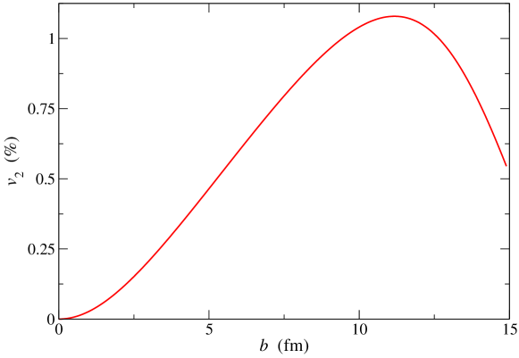
Figure 1: Centrality dependence of $v_{2}$ (here, for an evolution with on average 0.1 collision per particle).

3 Anisotropic initial momentum distribution, isotropic cross section

We now allow for the possibility that the expanding gas possess an initially anisotropic momentum distribution, which we describe by introducing its Fourier series

$$\tilde{f}({\bf p})=\tilde{f}_{0}(p_{T})\Bigg{[}1+2\sum_{k=1}^{\infty}\big{(}w_{k,c}\cos k\varphi+w_{k,s}\sin k\varphi\big{)}\Bigg{]}.$$ (17)

The Fourier coefficients $w_{k,c}$, $w_{k,s}$ could generally depend on $p_{T}$, yet we shall hereafter leave this dependence aside. The coefficients $w_{n,c}$ of the cosine harmonics correspond to the “usual” anisotropic flow coefficients, taken at the initial time, $v_{n}(t=0,p_{T})$. As in the previous Section, the differential cross section is taken to be isotropic.

The initial momentum distribution (17) gives for the unintegrated kernel

$${\cal C}({\bf v}t,{\bf p})=\frac{N_{c}N\tilde{f}_{0}(p_{T})}{8\pi^{2}R^{2}} \sqrt{1-\epsilon^{2}}\ {\rm e}^{-c^{2}t^{2}/4R^{2}}$$ (18)

$$\times\exp\!\left(\!-\frac{c^{2}t^{2}}{4R^{2}}\epsilon\cos 2\varphi\right)\!\Bigg{[}1+2\sum_{k=1}^{\infty}\big{(}w_{k,c}\cos k\varphi+w_{k,s}\sin k\varphi\big{)}\Bigg{]}.$$ (19)

With this kernel, the scattering rate is given by

$$\Gamma(t)=\frac{N_{c}N\sigma_{\rm el.}c}{4\pi R^{2}}\sqrt{1-\epsilon^{2}}\ {\rm e}^{-c^{2}t^{2}/4R^{2}}\,\Bigg{[}I_{0}\Bigg{(}\frac{c^{2}t^{2}}{4R^{2}}\epsilon\Bigg{)}+2\sum_{q\geq 1}(-1)^{q}w_{2q,c}I_{q}\Bigg{(}\frac{c^{2}t^{2}}{4R^{2}}\epsilon\Bigg{)}\Bigg{]},$$

and the total number of rescatterings, which has to be kept small, by

$${\cal N}_{\rm scat.}=\frac{N_{c}N\sigma_{\rm el.}}{4\sqrt{\pi}R}\,\sqrt{1-\epsilon^{2}}\,\Bigg{[}\,\! {}_{2}F_{1}\Bigg{(}\frac{1}{4},\frac{3}{4};1;\epsilon^{2}\Bigg{)}$$

$$+\sum_{q\geq 1}(-1)^{q}w_{2q,c}\frac{(2q\!-\!1)!!}{2^{2q-1}q!}\,_{2}F_{1}\Bigg{(}\frac{2q\!+\!1}{4},\frac{2q\!+\!3}{4};q\!+\!1;\epsilon^{2}\Bigg{)}\,\epsilon^{q}\Bigg{]}.$$

The unintegrated kernel (18) also allows one to compute the time derivative of the anisotropic flow coefficient $v_{n}$. As in Section 2, the gain term of the collision integral does not contribute to $\partial_{t}v_{n}(t,p_{T})$, whereas the contribution of the loss term follows from multiplying Equation (18) with $\cos n\varphi$ and then integrating over $\varphi$. The only terms from the sum over $k$ that result in a non-vanishing integral are those in $\cos k\varphi$ with $k$ of the same parity as $n$, so that $n-k$ and $n+k$ are even. The isotropic part of the momentum distribution only contributes when $n$ is even, as in Equation (14).

All in all, one finds

$$\partial_{t} v_{2m}(t,p_{T})\Big{|}_{\rm loss}\!=(-1)^{m+1}\frac{N_{c}\sigma_{\rm el.}c}{4\pi R^{2}} \sqrt{1-\epsilon^{2}}\ {\rm e}^{-c^{2}t^{2}/4R^{2}}\Bigg{\{}I_{m}\Bigg{(}\frac{c^{2}t^{2}}{4R^{2}}\epsilon\Bigg{)}$$ (20b)

$$\!\!\!+\!\sum_{q\geq 1}(-1)^{q}w_{2q,c}\Bigg{[}I_{m+q}\Bigg{(}\frac{c^{2}t^{2}}{4R^{2}}\epsilon\Bigg{)}\!+I_{m-q}\Bigg{(}\frac{c^{2}t^{2}}{4R^{2}}\epsilon\Bigg{)}\!\Bigg{]}\!\Bigg{\}},$$

$$\partial_{t} v_{2m+1}(t,p_{T})\Big{|}_{\rm loss}\!=(-1)^{m+1} \frac{N_{c}\sigma_{\rm el.}c}{4\pi R^{2}}\sqrt{1-\epsilon^{2}}\ {\rm e}^{-c^{2}t^{2}/4R^{2}}$$ (20d)

$$\times\sum_{q\geq 1}(-1)^{q}w_{2q-1,c}\Bigg{[}I_{m+q}\Bigg{(}\frac{c^{2}t^{2}}{4R^{2}}\epsilon\Bigg{)}\!+I_{m-q}\Bigg{(}\frac{c^{2}t^{2}}{4R^{2}}\epsilon\Bigg{)}\Bigg{]}.$$

Let us shortly discuss these results, focusing first on the short-time behaviour. Taking $m=1$, Equation (20b) gives for the evolution of elliptic flow

$$\partial_{t}v_{2}(t,p_{T})\sim\frac{N_{c}\sigma_{\rm el.}c}{4\pi R^{2}}\sqrt{1-\epsilon^{2}}\left[-w_{2,c}+\frac{c^{2}}{8R^{2}}\big{(}\epsilon+2w_{2,c}+\epsilon w_{4,c}\big{)}t^{2}+\Or(t^{4})\right]\ \mbox{ for }t\ll\frac{R}{c}.$$

That is, in the presence of a positive initial elliptic flow, $v_{2}(t,p_{T})$ first decreases (linearly), before it starts increasing: since more particles are emitted in-plane than out-of-plane, there are more particles “lost” at $\varphi=0$ or 180^o than at $\pm 90^{\rm o}$. On the contrary, a negative initial $w_{2,c}=v_{2}(0,p_{T})$ accelerates the initial increase of elliptic flow, while the later behaviour depends on the sign of $\epsilon(1+w_{4,c})+2w_{2,c}$. In either case, $v_{2}$ evolves even for vanishing eccentricity $\epsilon=0$, which is quite a nontrivial finding. One also sees that $v_{2}$ is influenced by the presence of any finite initial $w_{4,c}=v_{4}(0,p_{T})$.

For odd harmonics $n$, Equation (20d) shows that some finite $v_{n}(t,p_{T})$ can develop if and only if there exist at least one non-vanishing odd harmonic at $t=0$. In the case of directed flow $v_{1}$ for instance, Equation (20d) with $m=0$ gives

$$\partial_{t}v_{1}(t,p_{T}) =-\frac{N_{c}\sigma_{\rm el.}c}{2\pi R^{2}}\sqrt{1-\epsilon^{2}}\,{\rm e}^{-c^{2}t^{2}/4R^{2}}\sum_{q\geq 1}(-1)^{q}w_{2q-1,c}I_{q}\Bigg{(}\frac{c^{2}t^{2}}{4R^{2}}\epsilon\Bigg{)}$$

$$\sim\frac{N_{c}\sigma_{\rm el.}c^{3}}{16\pi R^{4}}\sqrt{1-\epsilon^{2}}\,w_{1,c}\epsilon t^{2}+\Or(t^{4})\ \mbox{ for }t\ll\frac{R}{c},$$

whereas for triangular flow $v_{3}$, one finds

$$\partial_{t}v_{3}(t,p_{T})\sim\frac{N_{c}\sigma_{\rm el.}c}{4\pi R^{2}}\sqrt{1-\epsilon^{2}}\left[-w_{1,c}+\frac{c^{2}}{8R^{2}}\big{(}w_{3,c}\epsilon+2w_{1,c}\big{)}t^{2}+\Or(t^{4})\right]\ \mbox{ for }t\ll\frac{R}{c}.$$

Thus, $v_{3}$ evolves even in the absence of any “triangularity” in the collision geometry—in obvious similarity to the evolution of $v_{2}$ for $\epsilon=0$. Additionally, $\partial_{t}v_{3}(t,p_{T})$ again illustrates the mixing of different harmonics present in Equations (20b)–(20d).

The latter can be integrated from $t=0$ to $\infty$. One in particular gets

$$v_{2}(p_{T})=w_{2,c}+ \frac{N_{c}\sigma_{\rm el.}\sqrt{1\!-\!\epsilon^{2}}}{16\sqrt{\pi}R}\,\Bigg{\{}{}_{2}F_{1}\Bigg{(}\frac{3}{4},\frac{5}{4};2;\epsilon^{2}\Bigg{)}\epsilon$$

$$\hskip 28.45274pt+\sum_{q\geq 1}\!\Bigg{(}\frac{-1}{4}\Bigg{)}^{\!\!q}w_{2q,c}\Bigg{[}\frac{(2q\!+\!1)!!}{(q\!+\!1)!}\,_{2}F_{1}\Bigg{(}\frac{2q\!+\!3}{4},\frac{2q\!+\!5}{4};q\!+\!2;\epsilon^{2}\Bigg{)}\epsilon^{q+1}$$

$$\hskip 128.0374pt+16\frac{|2q\!-\!3|!!}{(q\!-\!1)!}\,_{2}F_{1}\Bigg{(}\frac{2q\!-\!1}{4},\frac{2q\!+\!1}{4};q;\epsilon^{2}\Bigg{)}\epsilon^{q-1}\Bigg{]}\!\Bigg{\}}.$$

The initial elliptic flow $w_{2,c}=v_{2}(t\!=\!0,p_{T})$ breaks the linear scaling of $v_{2}$ with eccentricity at small $\epsilon$ both trivially as well as through its influence on the anisotropic flow developed in the rescatterings:

$$v_{2}(p_{T})\underset{\epsilon\ll 1}{\sim}\Bigg{(}1-\frac{N_{c}\sigma_{\rm el.}}{4\sqrt{\pi}R}\Bigg{)}v_{2}(t\!=\!0,p_{T})+\frac{N_{c}\sigma_{\rm el.}}{16\sqrt{\pi}R}\big{[}1+3v_{4}(t\!=\!0,p_{T})\big{]}\,\epsilon.$$

Again, we find the mixing of different harmonics as well as an evolving $v_{2}$ at $\epsilon=0$. Note that the ratio $N_{c}\sigma_{\rm el.}/4\sqrt{\pi}R$ necessarily takes a small value when the mean number of rescatterings per particle is small. Accordingly, $v_{2}(p_{T})$ does not differ much from its initial value, which is normal within our few-rescatterings approach.

4 Isotropic initial momentum distribution, anisotropic cross section

We now come back to an isotropic initial momentum distribution, but consider the case of an anisotropic differential cross section $\sigma_{\rm d}(\Theta)$. The latter can generally be expanded as a Fourier series. The first harmonic in the expansion describes an asymmetry between forward and backward scattering, the former being favored if the corresponding coefficient is positive. Then, the second harmonic accounts for increased or suppressed scattering at $\pm 90^{\rm o}$ with respect to 0 or 180^o. Higher harmonics describe less natural behaviours, which we shall not consider in the following. Additionally, we assume that the interaction preserves parity, so that sine harmonics vanish. We thus restrict ourselves to a differential cross section given by

$$\sigma_{\rm d}(\Theta)=\frac{\sigma_{\rm el.}}{2\pi}\big{(}1+2\varsigma_{1}\cos\Theta+2\varsigma_{2}\cos 2\Theta\big{)}.$$ (20u)

Note that the coefficients $\varsigma_{1}$ and $\varsigma_{2}$ are not totally arbitrary, since $\sigma_{\rm d}$ must remain non-negative when $\Theta$ spans the range $[0,2\pi]$: one for example easily checks that, irrespective of the value of $\varsigma_{1}$, one should have $|\varsigma_{2}|\leq\frac{1}{2}$.

The anisotropy of the differential cross section does not affect the scattering rate nor the resulting total number of rescatterings, which are thus given by Equations (11) and (12). The loss term of the collision integral relies on the total elastic cross section and is thus the same as in Section 2: it still yields a contribution to $\partial_{t}v_{n}(t,p_{T})$ given by the right-hand side of Equation (14).

On the other hand, the gain term of the collision integral now gives a non-vanishing contribution, since $\varphi^{\prime}$ is no longer arbitrary, but related to $\varphi$ through $\varphi^{\prime}=\varphi+\Theta$, with a non-uniform distribution in $\Theta$. Inspecting Equations (5), (10) and (13) together with the differential cross section (20u), the contribution to $\partial_{t}v_{n}(t,p)$ of the gain term reads

$$\partial_{t}v_{n}(t,p_{T})\Big{|}_{\rm gain}\!= \frac{N_{c}\sigma_{\rm el.}c}{8\pi^{2}R^{2}}\,\sqrt{1-\epsilon^{2}}\ {\rm e}^{-c^{2}t^{2}/4R^{2}}\$$

$$\times\!\int_{0}^{2\pi}\!{\rm d}\varphi\,\cos n\varphi\,\Bigg{\{}\!\int_{0}^{2\pi}\!\frac{{\rm d}\varphi^{\prime}}{2\pi}\, \!\exp\!\left(\!-\frac{c^{2}t^{2}}{4R^{2}}\epsilon\cos 2\varphi^{\prime}\right)$$

$$\!\times\!\Big{[}1+2\varsigma_{1}\cos(\varphi^{\prime}\!-\!\varphi)+2\varsigma_{2}\cos 2(\varphi^{\prime}\!-\!\varphi)\Big{]}\!\Bigg{\}}.$$

Irrespective of the value of $n$, the $\varsigma_{1}$ term leads to a vanishing integral over $\varphi^{\prime}$, while the integrals of the constant and $\varsigma_{2}$ terms yield modified Bessel functions, so that the expression between curly brackets equals

$$I_{0}\Bigg{(}\frac{c^{2}t^{2}}{4R^{2}}\epsilon\Bigg{)}-2\varsigma_{2}I_{1}\Bigg{(}\frac{c^{2}t^{2}}{4R^{2}}\epsilon\Bigg{)}\cos 2\varphi.$$

In turn, the remaining integral over $\varphi$ is trivial and yields for $n=2$

$$\partial_{t}v_{2}(t,p_{T})\Big{|}_{\rm gain}=-\frac{N_{c}\sigma_{\rm el.}c}{4\pi R^{2}}\sqrt{1-\epsilon^{2}}\,{\rm e}^{-c^{2}t^{2}/4R^{2}}\,I_{1}\Bigg{(}\frac{c^{2}t^{2}}{4R^{2}}\epsilon\Bigg{)}\varsigma_{2},$$

while it vanishes for $n\neq 2$, i.e. the gain term only contributes to the second harmonic of anisotropic flow, that is elliptic flow. Putting the gain and loss terms together, one eventually obtains after integrating over time

$$v_{2}(p_{T})=(1-\varsigma_{2})\frac{N_{c}\sigma_{\rm el.}\sqrt{1-\epsilon^{2}}}{16\sqrt{\pi}R}\,_{2}F_{1}\Bigg{(}\frac{3}{4},\frac{5}{4};2;\epsilon^{2}\Bigg{)}\,\epsilon,$$ (20v)

while $v_{n}(p_{T})$ for even $n\neq 2$ remains given by Equation (15). Thus, an increased (resp. decreased) scattering probability at $\pm 90^{\rm o}$, as found e.g. in collisions of identical bosons (resp. fermions)—which is obviously not the case of the colliding particles in our Lorentz-gas model—, leads to a larger (resp. smaller) $v_{2}$.

Eventually, one can mix the various ingredients together and consider an anisotropic differential cross section together with some initial anisotropic flow. In that case, the $\varsigma_{1}$ coefficient starts playing a role when combined with non-vanishing initial $w_{n,c}$, while $\varsigma_{2}$ will affect further flow harmonics besides $v_{2}$.

References

References

[1]
Heiselberg H and Levy A M 1999
Phys. Rev. C 59 2716
[2]
Borghini N and Gombeaud C 2011
Eur. Phys. J. C 71 1612
[3]
Krasnitz A, Nara Y and Venugopalan R 2003
Phys. Lett. B 554 21
[4]
Broniowski W, Florkowski W, Chojnacki M and Kisiel A 2009
Phys. Rev. C 80 034902
[5]
Prudnikov A P, Brychkov Yu A, Marichev O I 1992
Integrals and Series. vol.2: Special functions
(New York: Gordon and Breach)