Muon decay in orbit: spectrum of high-energy electrons

Abstract

Experimental searches for lepton-flavor-violating coherent muon-to-electron conversion in the field of a nucleus, have been proposed to reach the unprecedented sensitivity of $10^{-16}-10^{-18}$ per stopped muon. At that level, they probe new interactions at effective-mass scales well beyond 1000 TeV. However, they must contend with background from ordinary bound muon decay. To better understand the background-spectrum shape and rate, we have carried out a detailed analysis of Coulombic-bound-state muon decay, including nuclear recoil. Implications for future experiments are briefly discussed.

I Introduction and Motivation

From the observation of neutrino oscillations, we now know that lepton flavors (electron, muon and tau number) are not conserved. However, the mixing and small neutrino mass differences seen in oscillations have negligible effect on charged-lepton flavor violating (CLFV) reactions such as $\mu\to e\gamma$ or $\tau\to\mu\gamma$ (now predicted to occur with unobservable tiny branching ratios of about $10^{-54}$). So, if charged-lepton flavor violation were to be experimentally detected, it would have to come from “new physics” such as supersymmetry, heavy neutrino mixing, leptoquark interactions or some other extension of the Standard Model. In that way, charged-lepton number violating reactions provide a discovery window to interactions, beyond Standard Model expectations, reaching effective-mass scales above $\mathcal{O}(1000\,{\textrm{TeV}})$ Kuno:1999jp ; LeptMomBook .

Because muons can be copiously produced at accelerators and are relatively long lived ($2.2\text{ $\mu$}\mbox{s}$), they have been at the forefront of searches for CLFV Kuno:1999jp ; LeptMomBook . One reaction that can be probed with particularly high sensitivity is the muon-electron conversion in a muonic atom,

$$\mu^{-}+(A,Z)\to e^{-}+(A,Z),$$ (1)

where $(A,Z)$ represents a nucleus of atomic number $Z$ and mass number $A$. Various experiments have been performed over the years to search for this process Marciano:2008zz . The most recent, and stringent, results come from the SINDRUM II Collaboration Bertl:2006up , which reports an upper limit of $7\times 10^{-13}$ for the branching ratio of the conversion process relative to muon capture in gold, and a similar unpublished bound for titanium. Several new efforts are being planned. In the nearest future, the DeeMe Collaboration DeeMe has proposed to reach $10^{-14}$ sensitivity. Larger scale searches, Mu2e at Fermilab Carey:2008zz and COMET at J-PARC Cui:2009zz , aim for sensitivities below $10^{-16}$. In the long run, intensity upgrades at Fermilab and the proposal PRISM/PRIME at J-PARC may allow them to reach $10^{-18}$ sensitivity, a limit only accessible with muon-electron conversion in nuclei. For comparison, the current best upper bound on the branching ratio of the decay $\mu\to e\gamma$, set by the MEGA experiment, is $1.2\times 10^{-11}$ ($90\%$ confidence level) Brooks:1999pu . For some mechanisms of CLFV, the conversion process is less sensitive than $\mu\to e\gamma$ by a factor on the order of a few hundred Czarnecki:1998iz . But even in those cases, a $10^{-14}$ conversion search is more sensitive than this best current bound, and may be competitive with the new search for $\mu\to e\gamma$ by the MEG experiment Adam:2009ci . In addition, the conversion process is also sensitive to CLFV chiral-conserving amplitudes that do not contribute to $\mu\to e\gamma$.

The success of the conversion searches depends critically on control of the background events. The signal for the $\mu-e$ conversion process in Eq. (1) is a mono-energetic electron with energy $E_{\mu e}$, given by

$$E_{\mu e}=m_{\mu}-E_{\mathrm{b}}-E_{\mathrm{rec}},$$ (2)

where $m_{\mu}$ is the muon mass, $E_{\mathrm{b}}\simeq Z^{2}\alpha^{2}m_{\mu}/2$ is the binding energy of the muonic atom, and $E_{\mathrm{rec}}\simeq m_{\mu}^{2}/(2m_{N})$ is the nuclear-recoil energy, with $\alpha$ the fine-structure constant and $m_{N}$ the nucleus mass. The main physics background for this signal comes from the so-called muon decay in orbit (DIO), a process in which the muon decays in the normal way, i.e. $\mu^{-}\to e^{-}\bar{\nu}_{e}\nu_{\mu}$, while in the orbit of the atom. Whereas in a free muon decay, in order to conserve energy and three-momentum, the maximum electron energy is $m_{\mu}/2$, for decay in orbit the presence of an additional particle (the nucleus), which can absorb three-momentum, causes the maximum electron energy to be $E_{\mu e}$. Therefore, the high-energy tail of the electron spectrum in muon decay in orbit constitutes a background for conversion searches. A detailed study of that background is the main focus of this work.

Several theoretical studies of the muon decay in orbit have been performed, starting with Ref. Porter:1951zz about 60 years ago. Reference Haenggi:1974hp presented expressions which allow for a calculation of the electron spectrum including relativistic effects in the muon wavefunction, the Coulomb interaction between the electron and the nucleus and a finite nuclear size. Nuclear-recoil effects which, as we will discuss later, need to be considered in the high-energy region were only included in the Born approximation (that is, using the non-relativistic Schrödinger wave function for the muon and a plane wave for the electron), which is not adequate for the high-energy tail. Later, Refs. Watanabe:1987su ; Watanabe:1993 presented similar expressions for the electron spectrum completely neglecting nuclear-recoil effects, evaluating it for several different elements. None of these references focused on the high-energy endpoint of the spectrum, which is the region of interest for conversion experiments. References Shanker:1981mi ; Shanker:1996rz did study the high-energy end of the electron spectrum, and presented approximate results which allow for a quick rough estimate of the muon decay in orbit contribution to the background in conversion experiments. However, a detailed evaluation of the high-energy region of the electron spectrum is still missing in the literature. What is typically done, to account for the background from muon decay in orbit, is to connect (in a somewhat arbitrary way) the approximate expressions given in Ref. Shanker:1981mi with the numerical results presented in Ref. Watanabe:1993 . Since this is the main source of background Carey:2008zz ; Cui:2009zz for the oncoming conversion experiments, a more detailed analysis is highly desirable. In this work we discuss all the relevant effects that need to be included in the high-energy region of the spectrum and present a precise evaluation of it. Our results for an aluminum ($Z=13$) nucleus (the intended target in Mu2e and COMET) are presented in Figure 1.

The structure of the paper is as follows. In Sec. II we present the formulae for the computation of the electron spectrum. In Sec. III we describe the numerical evaluation of the spectrum. Section IV contains some discussion on the different contributions in the high-energy region of the spectrum, and the approximations we have used. We conclude in Sec. V, where brief comments regarding the implications of our results are given. Appendix A details the conventions we use for the Dirac equation, and the electron and muon wavefunctions.

II Formulae for the electron spectrum

The Fermi interaction that mediates muon decay is given by

$$\mathcal{L}_{F}=-2\sqrt{2}G_{F}\left[\bar{\psi}_{\nu_{\mu}}\gamma^{\rho}P_{L}\psi_{\mu}\right]\left[\bar{\psi}_{e}\gamma_{\rho}P_{L}\psi_{\nu_{e}}\right]+\textrm{h.c.},$$ (3)

where $G_{F}=1.1663788(7)\times 10^{-5}\,\textrm{GeV}^{-2}$ is the Fermi constant and $P_{L}=(1-\gamma_{5})/2$. This Lagrangian can be Fierz rearranged to charge-retention ordering,

$$\mathcal{L}_{F}=2\sqrt{2}G_{F}\left[\bar{\psi}_{e}\gamma^{\rho}P_{L}\psi_{\mu}\right]\left[\bar{\psi}_{\nu_{\mu}}\gamma_{\rho}P_{L}\psi_{\nu_{e}}\right]+\textrm{h.c.},$$ (4)

which is the form that we will use. Since quantum electrodynamics (QED) interactions do not affect the neutrino part of the Lagrangian, it is convenient to partition the phase space and integrate the neutrino portion. In that way, we generate an effective $\mu-e$ current and the free muon decay rate can be written as

$$\Gamma=\frac{1}{2E_{\mu}}\int dq^{2}\int\left[d\Pi_{\mu\to eq}\right]\left|\mathcal{M}_{\mu\to e}^{\rho\sigma}\right|^{2}T_{\rho\sigma},$$ (5)

with

$$d\Pi_{\mu\to eq} \equiv \int\frac{d^{3}p_{e}}{(2\pi)^{3}2E_{e}}\int\frac{d^{3}k}{(2\pi)^{3}2E_{q}}(2\pi)^{4}\delta^{(4)}(p_{\mu}-p_{e}-q),$$

$$T_{\rho\sigma} \equiv -\frac{\pi}{3(2\pi)^{3}}\left(q^{2}g_{\rho\sigma}-q_{\rho}q_{\sigma}\right),$$

$$\left|\mathcal{M}_{\mu\to e}^{\rho\sigma}\right|^{2} \equiv \frac{1}{2}\sum_{\mu^{-}\,\textrm{\tiny spin}}\,\sum_{e^{-}\,\textrm{\tiny spin}}8G_{F}^{2}\bar{u}(p_{e})\gamma^{\rho}P_{L}u(p_{\mu})\bar{u}(p_{\mu})\gamma^{\sigma}P_{L}u(p_{e}),$$ (6)

where the spinors $u(p)$ in that expression are normalized according to $\bar{u}^{r}(p)u^{s}(p)=2m\delta^{rs}$, $q_{\rho}\equiv(E_{q},\vec{k})$ is the 4-momentum transferred to the neutrinos, $\vec{p}_{e}$ is the electron three-momentum and $E_{e}$ and $E_{\mu}$ are the electron and muon energies, respectively. When we consider the bound muon decay case, Eq. (5) gets replaced by

$$\Gamma = \frac{2G_{F}^{2}}{(2\pi)^{6}}\sum_{e^{-}\,\textrm{\tiny spin}}\int dq^{2}\frac{d^{3}p_{e}}{E_{e}^{2}}\frac{d^{3}k}{E_{q}}(2\pi)\delta(E_{\mu}-E_{e}-E_{q})$$ (7)

$$\times\left[\int d^{3}re^{-i\vec{k}\cdot\vec{r}}\bar{\varphi}_{e}\gamma^{\rho}P_{L}\varphi_{\mu}\right]\left[\int d^{3}r^{\prime}e^{i\vec{k}\cdot\vec{r}^{\prime}}\bar{\varphi}_{\mu}\gamma^{\sigma}P_{L}\varphi_{e}\right]T_{\rho\sigma},$$

where we are taking the nucleus as static (we discuss the inclusion of recoil effects in the next Section), and $\varphi_{e}$ and $\varphi_{\mu}$ represent the solutions of the Dirac equation for the electron and the muon, respectively. We incorporate the average over the muon spin in the definition of $\varphi_{\mu}$, while we do not incorporate the sum over the electron spin in the definition of $\varphi_{e}$. For the normalization convention that is implied for the wavefunctions in Eq. (7) we refer to Appendix A. The muon energy in Eq. (7) is given by $E_{\mu}=m_{\mu}-E_{\mathrm{b}}$. When the muonic atom is formed, the muon cascades down almost immediately to the ground state, the $1S$ wavefunction should therefore be used for $\varphi_{\mu}$ in Eq. (7) (the cascade process also depolarizes the muons :2009yn ). We take the electron to be massless, since electron mass effects are only relevant for $E_{e}\sim m_{e}$, which is not our region of interest. Integrating over $dq^{2}$ in Eq. (7) we obtain

$$\Gamma=-\sum_{e^{-}\,\textrm{\tiny spin}}\frac{G_{F}^{2}}{192\pi^{7}}\int\frac{d^{3}p_{e}}{E_{e}^{2}}\int d^{3}kJ^{\rho}J^{\sigma\dagger}\left(q^{2}g_{\rho\sigma}-q_{\rho}q_{\sigma}\right),$$ (8)

where it is understood that $q_{\rho}=(E_{\mu}-E_{e},\vec{k})$, and we defined

$$J^{\rho}\equiv\int d^{3}re^{-i\vec{k}\cdot\vec{r}}\bar{\varphi}_{e}\gamma^{\rho}P_{L}\varphi_{\mu}.$$ (9)

The condition $q^{2}>0$ determines the limit of integration for $|\vec{k}|$ to be $|\vec{k}|<E_{\mu}-E_{e}$. Performing the angular integration over $\vec{r}$ in the currents $J^{\rho}$, and the angular integrations over $\vec{k}$ and $\vec{p}_{e}$ and summing over electron spins in Eq. (8) we obtain

$$\frac{1}{\Gamma_{0}}\frac{d\Gamma}{dE_{e}} = \sum_{K\kappa}\frac{4}{\pi m_{\mu}^{5}}(2j_{\kappa}+1)\int_{0}^{E_{\mu}-E_{e}}\!\!\!\!\!\!\!\!\!\!dk\,k^{2}$$ (10)

$$\times\Bigg{\{}\left[(E_{\mu}-E_{e})^{2}-k^{2}\right]\left(\frac{|S_{K\kappa}^{0}|^{2}}{K(K+1)}+\frac{|S_{K\kappa}^{-1}|^{2}}{K(2K+1)}+\frac{|S_{K\kappa}^{+1}|^{2}}{(K+1)(2K+1)}\right)$$

$$+\left[(E_{\mu}-E_{e})k\right]2\textrm{Im}\!\!\left(\frac{S_{K\kappa}\left(S^{-1\,*}_{K\kappa}+S^{+1\,*}_{K\kappa}\right)}{2K+1}\right)+k^{2}\left(\frac{|S^{-1}_{K\kappa}+S^{+1}_{K\kappa}|^{2}}{(2K+1)^{2}}+|S_{K\kappa}|^{2}\right)\!\Bigg{\}},$$

where

$$\Gamma_{0}\equiv\frac{G_{F}^{2}m_{\mu}^{5}}{192\pi^{3}},$$ (11)

is the free-muon decay rate. The $S$ functions in Eq. (10) are defined using the notation $\left\langle\ldots\right\rangle\equiv\int_{0}^{\infty}\ldots r^{2}dr$, and the two cases refer to odd/even $l_{\kappa}+K$, respectively

$$S_{K\kappa}^{0} = \begin{cases}-i\left(\kappa-1\right)\left\langle j_{K}(kr)\left(f_{\kappa}G+g_{\kappa}F\right)\right\rangle\\ \left(\kappa+1\right)\left\langle j_{K}(kr)\left(g_{\kappa}G-f_{\kappa}F\right)\right\rangle\end{cases},$$

$$S_{K\kappa}^{-1} = \begin{cases}\left\langle j_{K-1}(kr)\left[(\kappa-K-1)g_{\kappa}G-(\kappa+K-1)f_{\kappa}F\right]\right\rangle\\ -i\left\langle j_{K-1}(kr)\left[(\kappa+K+1)f_{\kappa}G+(\kappa-K+1)g_{\kappa}F\right]\right\rangle\end{cases},$$

$$S_{K\kappa}^{+1} = \begin{cases}\left\langle j_{K+1}(kr)\left[(\kappa+K)g_{\kappa}G+(K-\kappa+2)f_{\kappa}F\right]\right\rangle\\ -i\left\langle j_{K+1}(kr)\left[(\kappa-K)f_{\kappa}G+(\kappa+K+2)g_{\kappa}F\right]\right\rangle\end{cases},$$

$$S_{K\kappa} = \begin{cases}i\left\langle j_{K}(kr)(f_{\kappa}G-g_{\kappa}F)\right\rangle\\ \left\langle j_{K}(kr)\left(g_{\kappa}G+f_{\kappa}F\right)\right\rangle\end{cases},$$ (12)

where $G$ and $F$ ($g_{\kappa}$ and $f_{\kappa}$) are the upper and lower components of the radial muon (electron) wavefunction, respectively. $\kappa$ is the quantum number appearing in the Dirac equation (see Appendix A for the conventions we use and the definitions of $j_{\kappa}$ and $l_{\kappa}$). For a given value of $K$ in Eq. (10), $\kappa$ can only take the values $\pm K$ and $\pm(K+1)$. The sum over $K$ goes from 0 to $\infty$, but $K$ cannot take the value $K=0$ in the $S^{0}_{K\kappa}$ and $S^{-1}_{K\kappa}$ terms, and $\kappa$ can never be equal to 0. $j_{n}(z)$ is the spherical Bessel function of order $n$. Equation (10) agrees with the expressions presented in Refs. Watanabe:1987su ; Watanabe:1993 .

II.1 Inclusion of recoil effects

In the previous Section we considered the nucleus to be static. The upcoming conversion experiments plan to use an aluminum target (previous conversion experiments used heavier elements), where the atomic mass of aluminum ($Z=13$, $A=27$) is $25133\,\textrm{MeV}$. The nucleus is, therefore, more than 200 times heavier than the muon ($m_{\mu}=105.6584\,\textrm{MeV}$) and recoil effects should be negligible for most of the electron spectrum. However, the nuclear-recoil energy modifies the endpoint of the electron spectrum $E_{\mu e}$, see Eq. (2), which means that recoil effects need to be carefully considered in studies of the high-energy part of the spectrum. We will always consider the recoil effects at first order in a $1/m_{N}$ expansion, where $m_{N}$ is the mass of the nucleus $N$.

For muon DIO, the nuclear-recoil energy is

$$E_{\mathrm{rec}}=\frac{|\vec{p}_{N}|^{2}}{2m_{N}},$$ (13)

where the three-momentum of the nucleus is

$$\vec{p}_{N}=-\vec{p}_{e}-\vec{p}_{\bar{\nu}_{e}}-\vec{p}_{\nu_{\mu}},$$ (14)

with $\vec{p}_{\nu_{\mu}}$ and $\vec{p}_{\bar{\nu}_{e}}$ the three-momenta of the neutrino and anti-neutrino, respectively. We see that, for a given electron energy, the nuclear-recoil energy is not constant but depends on the momenta of the neutrinos. This complicates the integration over the neutrino momenta, but in the high-energy end of the spectrum we can approximate

$$E_{\mathrm{rec}}=\frac{\left|\vec{p}_{N}\right|^{2}}{2m_{N}}=\frac{\left(\vec{p}_{e}+\vec{p}_{\bar{\nu}_{e}}+\vec{p}_{\nu_{\mu}}\right)^{2}}{2m_{N}}\simeq\frac{\left|\vec{p}_{e}\right|^{2}}{2m_{N}}=\frac{E_{e}^{2}}{2m_{N}},$$ (15)

so that the recoil effects amount to a change in the momentum transfer to the neutrinos. The net effect is to substitute

$$E_{\mu}-E_{e}\to E_{\mu}-E_{e}-\frac{E_{e}^{2}}{2m_{N}},$$ (16)

in the upper limit of the integration over $k$ and inside the square brackets in Eq. (10). The endpoint of the electron spectrum is given by

$$E_{\mu e}=E_{\mu}-\frac{E_{\mu}^{2}}{2m_{N}}=m_{\mu}-E_{\mathrm{b}}-\frac{E_{\mu}^{2}}{2m_{N}},$$ (17)

which is exact up to corrections of order $1/m_{N}^{2}$. The approximation for the recoil energy in Eq. (15) is the same as used in Ref. Shanker:1981mi . The electron spectrum including nuclear-recoil effects is, therefore, given by

$$\frac{1}{\Gamma_{0}}\frac{d\Gamma}{dE_{e}} = \sum_{K\kappa}\frac{4}{\pi m_{\mu}^{5}}(2j_{\kappa}+1)\int_{0}^{E_{\mu}-E_{e}-\frac{E_{e}^{2}}{2m_{N}}}\!\!\!\!\!\!\!\!\!\!dk\,k^{2}$$ (18)

$$\times\Bigg{\{}\left[\left(E_{\mu}-E_{e}-\frac{E_{e}^{2}}{2m_{N}}\right)^{2}\!\!\!-k^{2}\right]\!\left(\frac{|S_{K\kappa}^{0}|^{2}}{K(K+1)}+\frac{|S_{K\kappa}^{-1}|^{2}}{K(2K+1)}+\frac{|S_{K\kappa}^{+1}|^{2}}{(K+1)(2K+1)}\right)$$

$$+2k\left(E_{\mu}-E_{e}-\frac{E_{e}^{2}}{2m_{N}}\right)\textrm{Im}\frac{S_{K\kappa}\left(S_{K\kappa}^{-1\,*}+S_{K\kappa}^{+1\,*}\right)}{2K+1}$$

$$+k^{2}\left(\frac{|S_{K\kappa}^{-1}+S_{K\kappa}^{+1}|^{2}}{(2K+1)^{2}}+|S_{K\kappa}|^{2}\right)\!\Bigg{\}},$$

where it is understood that this expression should only be used in the region where Eq. (15) is a good approximation to the nuclear-recoil energy. As will be manifest in the following Sections, recoil effects become negligible before Eq. (15) ceases to be a good approximation to the recoil energy. That means the inclusion of recoil effects beyond the approximation considered here is unnecessary.

II.2 Endpoint expansions

Equation (18) constitutes our final result for the high-energy region of the electron spectrum and it is what we will use in our numerical evaluations. Nevertheless, it is still interesting to perform a Taylor expansion of Eq. (18) around the endpoint, to make the behavior of the spectrum manifest. We obtain

$$\left.\frac{1}{\Gamma_{0}}\frac{d\Gamma}{dE_{e}}\right|_{E_{e}\sim E_{\mu}-\frac{E_{\mu}^{2}}{2m_{N}}} = \frac{64}{5\pi m_{\mu}^{5}}\left(E_{\mu}-E_{e}-\frac{E_{e}^{2}}{2m_{N}}\right)^{5}\left(p_{1}^{2}+\frac{s_{1}^{2}}{3}+\frac{2}{3}r_{2}^{2}\right)$$ (19)

$$\equiv B\left(E_{\mu}-E_{e}-\frac{E_{e}^{2}}{2m_{N}}\right)^{5},$$

where $p_{\kappa}=\left\langle g_{-\kappa}G\right\rangle$, $s_{\kappa}=\left\langle f_{-\kappa}F\right\rangle,$ $r_{\kappa}=\left\langle g_{-\kappa}F\right\rangle$, and it is understood that the electron wavefunctions $g_{\kappa}$ and $f_{\kappa}$ in Eq. (19) correspond to the energy $E_{e}=E_{\mu}-E_{\mu}^{2}/(2m_{N})$. We show the values of the $B$ coefficient in Eq. (19), for a few elements, in Table 1.

Table 1: Values for the $B$ coefficient of the leading-order Taylor expansion in Eq. (19), for a few elements. We use finite-size nuclei, characterized by a two-parameter Fermi distribution (see Eq. (21)), with the values of the parameters of that distribution taken from Refs. De Jager:1987qc ; Fricke:1995zz .

Nucleus	$B(\,\textrm{MeV}^{-6})$
Al($Z=13$)	$8.98\times 10^{-17}$
Ti($Z=22$)	$4.94\times 10^{-16}$
Cu($Z=29$)	$1.14\times 10^{-15}$
Se($Z=34$)	$1.62\times 10^{-15}$
Sb($Z=51$)	$3.57\times 10^{-15}$
Au($Z=79$)	$4.79\times 10^{-15}$

The corresponding Taylor expansion for the expression without recoil effects in Eq. (10) is given by

$$\left.\frac{1}{\Gamma_{0}}\frac{d\Gamma}{dE_{e}}\right|_{E_{e}\sim E_{\mu}}^{\textrm{\tiny no recoil}}=\frac{64}{5\pi m_{\mu}^{5}}(E_{\mu}-E_{e})^{5}\left(p_{1}^{2}+\frac{s_{1}^{2}}{3}+\frac{2}{3}r_{2}^{2}\right),$$ (20)

where it is understood that the electron wavefunctions in this equation correspond to the energy $E_{e}=E_{\mu}$. Our Taylor expansion agrees with the results in Ref. Shanker:1981mi .

III Numerical evaluation of the spectrum

We now use Eq.(18) to obtain a numerical evaluation of the high-energy region of the electron spectrum. We present the results for the case of an aluminum nucleus (Al, $Z=13$), which is the target intended to be used in Mu2e and COMET Carey:2008zz ; Cui:2009zz .

We consider a nucleus of finite size, characterized by a two-parameter Fermi distribution $\rho(r)$, given by

$$\rho(r)=\rho_{0}\frac{1}{1+e^{\frac{r-r_{0}}{a}}}.$$ (21)

For the parameters of the Fermi distribution we use the values De Jager:1987qc

$$r_{0}=2.84\pm 0.05\,\textrm{fm},\quad a=0.569\,\textrm{fm}.$$ (22)

$\rho_{0}$ in Eq. (21) is the normalization factor, which can be expressed in terms of $r_{0}$ and $a$. For the muon mass, aluminum mass and the fine-structure constant we use the values $m_{\mu}=105.6584\,\textrm{MeV},\text{ }m_{\textrm{\tiny Al}}=25133\,\textrm{MeV},\text{ }\alpha=\frac{1}{137.036},$ and remember that we take the electron to be massless. We numerically solve the radial Dirac equations for the muon and the electron, with the charge distribution in Eq. (21), to obtain the wavefunctions. For the muon energy we obtain

$$E_{\mu}=m_{\mu}-E_{\textrm{b}}=105.194\,\textrm{MeV},$$ (23)

which gives the endpoint energy

$$E_{\mu e}=E_{\mu}-\frac{E_{\mu}^{2}}{2m_{\textrm{\tiny Al}}}=104.973\,\textrm{MeV}.$$ (24)

Electron screening will increase the end-point energy in Eq. (24) by about $+0.001\,{\textrm{M}eV}$ and similarly shift the overall spectrum. That small effect is negligible for our considerations. Recall that the sum over $K$ in Eq. (18) goes from 0 to $\infty$, we include as many terms in $K$ as necessary in order to get three-digit precision for each point of the spectrum. This requires about 30 terms near $m_{\mu}/2$ and fewer terms in the low- and the high-energy parts of the spectrum.

We present the result of the numerical evaluation of the high-energy region of the electron spectrum in Fig 1. The squares in the figure are the spectrum with recoil effects, from Eq. (18). For comparison, we also show the result obtained by neglecting recoil effects, from Eq. (10), as the triangles. The right plot in the figure is a zoom for $E_{e}>100\,\textrm{MeV}$, the solid and dashed lines on this plot correspond to the Taylor expansions in Eqs. (19) and (20), respectively. Terms up to $K=4$ were included in Fig. 1. Figure 2 presents a detail of the electron spectrum very close to the high-energy endpoint in linear scale. We can appreciate in that figure how the spectra with (solid line) and without (dashed line) recoil effects tend to zero at the corresponding endpoints (the endpoint without recoil is at $E_{e}=E_{\mu}$).

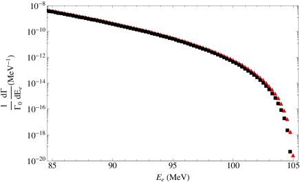
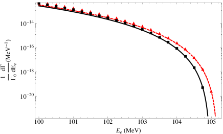
Figure 1: Endpoint region of the electron spectrum for aluminum. The squares correspond to the spectrum with recoil effects, Eq. (18). For comparison, we show the spectrum neglecting recoil, Eq. (10), as the triangles. The right plot is a zoom for $E_{e}>100\,\textrm{MeV}$, the solid (dashed) line on this plot corresponds to the Taylor expansion around the endpoint with (without) recoil.

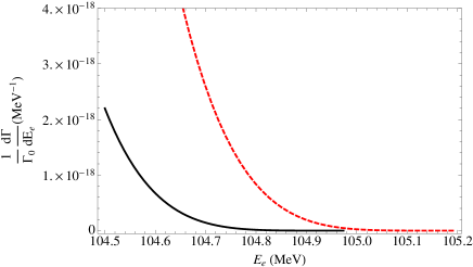
Figure 2: Detail of the electron spectrum for aluminum very close to the high-energy endpoint with (neglecting) nuclear recoil, represented as the solid (dashed) line.

To make our results easier to use, we mention that the polynomial

$$P(E_{e})\equiv a_{5}\delta^{5}+a_{6}\delta^{6}+a_{7}\delta^{7}+a_{8}\delta^{8},$$ (25)

with

$$a_{5}=8.6434\times 10^{-17},\,a_{6}=1.16874\times 10^{-17},\,a_{7}=-1.87828\times 10^{-19},\,a_{8}=9.16327\times 10^{-20},$$ (26)

the energies expressed in MeV, and

$$\delta=E_{\mu}-E_{e}-\frac{E_{e}^{2}}{2m_{\textrm{\tiny Al}}},$$ (27)

fits very well the result for the electron spectrum in aluminum normalized to the free decay rate (squares in Fig. 1) for all $E_{e}>85\,\textrm{MeV}$ (i.e., the difference between Eq. (25) and the squares in Fig. 1 is not larger than the uncertainties discussed in the next Section). Note that, in order to obtain a better fit for the whole $E_{e}>85$ MeV region, the value of $a_{5}$, in Eq. (25), was not constrained to be that of the leading coefficient of the Taylor expansion in Table 1.

For completeness, we also show the spectrum for the full range of electron energies in Fig. 3 as the circles, from Eq. (10). Terms up to $K=31$ were included in this plot.

Figure 3: Electron spectrum for aluminum. Left plot: linear scale; right plot: logarithmic scale.

The total decay rate for muon decay in orbit in aluminum is obtained by integrating the spectrum in Fig. 3. The result we obtain is

$$\frac{1}{\Gamma_{0}}\int_{0}^{E_{\mu e}}\frac{d\Gamma}{dE_{e}}dE_{e}=0.9934,$$ (28)

in agreement with Ref. Watanabe:1993 . Nuclear-recoil effects are negligible in the total rate. Also note, the integrated ordinary muon decay rate is hardly affected by the presence of the Coulomb potential, in accord with the general results in Uberall:1960zz ; Czarnecki:1999yj .

Since the Mu2e Collaboration also considers titanium (Ti, $Z=22$) as a viable target Carey:2008zz , we give the polynomial, $P^{(\textrm{\tiny Ti})}(E_{e})$, that fits the result for the electron spectrum in titanium (normalized to the free decay rate) for energies $E_{e}>85\,\textrm{MeV}$,

$$P^{(\textrm{\tiny Ti})}(E_{e})\equiv a_{5}^{(\textrm{\tiny Ti})}\delta_{(\textrm{\tiny Ti})}^{5}+a_{6}^{(\textrm{\tiny Ti})}\delta_{(\textrm{\tiny Ti})}^{6}+a_{7}^{(\textrm{\tiny Ti})}\delta_{(\textrm{\tiny Ti})}^{7}+a_{8}^{(\textrm{\tiny Ti})}\delta_{(\textrm{\tiny Ti})}^{8},$$ (29)

with

$$a_{5}^{(\textrm{\tiny Ti})}=4.44278\times 10^{-16},\,a_{6}^{(\textrm{\tiny Ti})}=9.06648\times 10^{-17},\,a_{7}^{(\textrm{\tiny Ti})}=-4.26245\times 10^{-18},\,a_{8}^{(\textrm{\tiny Ti})}=8.193\times 10^{-19},$$ (30)

the energies expressed in MeV,

$$\delta_{(\textrm{\tiny Ti})}=E_{\mu}-E_{e}-\frac{E_{e}^{2}}{2m_{\textrm{\tiny Ti}}},$$ (31)

and for titanium $E_{\mu}=104.394\,\textrm{MeV}$.

IV Discussion

As expected, the results in Figure 1 show that nuclear-recoil effects are only important close to the high-energy endpoint of the spectrum. The corrections to the approximation of the recoil energy that we have used in Eq. (15) are of order $E_{e}(E_{\mu}-E_{e})/(2m_{N})$ (while Ref. Shanker:1981mi seems to wrongly estimate this correction as being smaller $\sim\left(E_{\mu}-E_{e}\right)^{2}/(2m_{N})$). For electron energies around $85\,\textrm{MeV}$, Eq. (15) is still a good approximation to the recoil energy while the effect of recoil in the spectrum is very small. When the corrections to the approximation in Eq. (15) become order one, the recoil effects on the spectrum are negligible. Therefore we conclude that, as anticipated in Sec. II.1, inclusion of recoil effects beyond the approximation considered here is unnecessary.

As already noted in Ref. Shanker:1981mi , the Schrödinger wave function for the muon is not a good approximation near the endpoint. In that region, one needs to produce an electron with $E_{e}\sim|\vec{p}_{e}|\sim m_{\mu}$. This implies that, either the muon has $|\vec{p}_{\mu}|\sim m_{\mu}$ (i.e., it is at the tail of the wavefunction) or (if the muon has the typical atomic non-relativistic momentum, of order the inverse Bohr radius) the electron must interact with the nucleus to get $|\vec{p}_{e}|\sim m_{\mu}$. Those two contributions are of the same order in $\alpha$, which means that we cannot treat the muon within a non-relativistic approximation. There are, thus, some leading contributions where the muon is far off-shell (it has $E_{\mu}\sim|\vec{p}_{\mu}|\sim m_{\mu}$), a fact that also tells us that this is the region where finite-nuclear-size effects will be most important (since the muon will be closer to the nucleus). By this argument, we can also understand that only the lowest values of the angular momentum in the electron wavefunctions contribute at the endpoint (as we see in Eq. (19)).

Uncertainties in the modeling of finite nuclear-size effects can induce errors in the electron spectrum and, as we discussed in the previous paragraph, those are expected to be most important in the endpoint region. We re-computed the spectrum varying the parameters in the Fermi distribution as indicated in Eq. (22), and found that the errors induced in the spectrum do increase as we approach the endpoint, as expected, but they are never larger than $\pm 2\%$; so, we can safely ignore them.

Finally we comment that radiative corrections have not been included in Eq. (18). However, they are not expected to significantly modify the results presented.

V Conclusions and Experimental Applications

Figure 4: Total rate of decay-in-orbit events, for aluminum, with electron energy larger than $x$, normalized to the free muon decay rate $\Gamma_{0}$.

We have performed a detailed evaluation of the high-energy region of the electron spectrum in muon decay in orbit. Our results in Eq. (18), Eq. (25) and Figure 1 include all the relevant effects to accurately describe the high-energy region of the spectrum, and provide the correct background contribution for $\mu-e$ conversion search experiments. To summarize our findings, we plot in Fig. 4 the rate of decay in orbit events producing an electron with energy higher than $x$, as a function of $x$ (normalized to the free muon decay rate).

The complete muon DIO electron spectrum presented here provides a check on previous low- and high-energy partial calculations Watanabe:1993 ; Shanker:1981mi , as well as an interpolation between them. It properly incorporates recoil and relativistic effects in the high-energy endpoint region, which is of crucial importance for future $\mu-e$ conversion background studies. In that regard, its primary utility is twofold. First, when experimental data on muon DIO becomes available, our formula in Eq. (25) can be compared with it and used to refine the detector’s acceptance, efficiency and resolution. Second, the expected spectrum can be convoluted with the spectrometer resolution function to obtain a more precise estimate of the muon DIO background to CLFV $\mu-e$ conversion in the $E_{e}\simeq 103.5-105$ MeV signal region.

Currently available estimates by the Mu2e Collaboration Carey:2008zz find for $4\times 10^{16}$ ordinary muon captures in Al (corresponding to a total of $2.6\times 10^{16}$ DIO) a signal of 4 conversion events if $R_{\mu\mathrm{Al}}\equiv\Gamma\left(\mu^{-}\mathrm{Al}\to e^{-}\mathrm{Al}\right)/\Gamma\left(\mu^{-}\mathrm{Al}\to\nu_{\mu}\mathrm{Mg}\right)=10^{-16}$, with only about 0.2 DIO background events for their detector resolution function. At that level, the discovery capability is quite robust. However, if $R_{\mu\mathrm{Al}}$ is much smaller, more running will be required to enhance the signal and refinements of the background using the spectrum in Eq. (25) will be critical.

One can also use our analysis to make a rough comparison of DIO backgrounds for stopping targets with different $Z$. Indeed, if a signal for $\mu\to e$ conversion is found in Al, other targets will be important for extracting the underlying “new physics” responsible for it. Of course, for much higher $Z$, the initial dead time of 700 ns envisioned in the Mu2e proposal for eliminating prompt backgrounds would significantly reduce the number of “live” muon captures and severely compromise the experimental sensitivity. Ignoring that issue for now, we can ask: What DIO background is expected for a higher-$Z$ target with energy resolution identical to the Al setup of Mu2e, while continuing to require that it also produces 4 signal events? Considering the case of a titanium target, with $Z=22$, we expect $R_{\mu\mathrm{Ti}}\simeq 1.6R_{\mu\mathrm{Al}}$ for models of “new physics” Marciano:2008zz dominated by chiral changing CLFV. So, one needs a “live” run with “only” $2.5\times 10^{16}$ ordinary muon captures or correspondingly $0.43\times 10^{16}$ total DIO events to reach the same 4 event discovery sensitivity as in aluminum. However, even though the total number of DIO events (for all $E_{e}$) is smaller by a factor of 6 in Ti, the relative branching fraction for high-energy DIO events in the signal region (with similar detector resolution) is about 6 times larger for Ti compared to Al. So, overall the DIO background is about the same for Ti.

More difficult will be the loss of muon events in higher $Z$ materials due to the 700 ns dead time during which most of the muons undergo capture. For that, a complete reassessment of the muon production and stopping conditions may be required.

Appendix A Conventions

In this Appendix we explain our conventions for the Dirac equation, and the electron and muon wavefunctions.

The Dirac equation in a central field is given by

$$W\psi=\left[-i\gamma_{5}\sigma_{r}\left(\frac{\partial}{\partial r}+\frac{1}{r}-\frac{\beta}{r}K\right)+V(r)+m\beta\right]\psi,$$ (32)

where $W$ is the energy of the particle, $m$ its mass and $V(r)$ is the potential. The $4\times 4$ matrices $\gamma_{5}$, $\beta$, $K$ and $\sigma_{r}$ are given by

$$\gamma_{5}=\left(\begin{array}[]{cc}0&1\\ 1&0\end{array}\right)\,,\,\beta=\left(\begin{array}[]{cc}1&0\\ 0&-1\end{array}\right)\,,\,r\sigma_{r}=\left(\begin{array}[]{cc}\vec{\sigma}\cdot\vec{r}&0\\ 0&\vec{\sigma}\cdot\vec{r}\end{array}\right)\,,\,K=\left(\begin{array}[]{cc}\vec{\sigma}\cdot\vec{l}+1&0\\ 0&-(\vec{\sigma}\cdot\vec{l}+1)\end{array}\right),$$ (33)

with $\vec{l}$ the orbital angular momentum $\vec{l}=-i\vec{r}\times\vec{\nabla}$ and $\vec{\sigma}$ the $2\times 2$ Pauli matrices

$$\sigma_{x}=\left(\begin{array}[]{cc}0&1\\ 1&0\end{array}\right)\,,\,\sigma_{y}=\left(\begin{array}[]{cc}0&-i\\ i&0\end{array}\right)\,,\,\sigma_{z}=\left(\begin{array}[]{cc}1&0\\ 0&-1\end{array}\right).$$ (34)

The wavefunctions are generically denoted as follows

$$\psi=\psi_{\kappa}^{\mu}=\left(\begin{array}[]{c}g_{\kappa}(r)\chi_{\kappa}^{\mu}\\ if_{\kappa}(r)\chi_{-\kappa}^{\mu}\end{array}\right),$$ (35)

they diagonalize the operators $K$, $\vec{j}^{2}$ and $j_{z}$ ($\vec{j}$ being the total angular momentum) with eigenvalues $-\kappa$, $j(j+1)$ and $\mu$, respectively. $g_{\kappa}$ and $f_{\kappa}$ are the radial functions which are given by the equations

$$\frac{df_{\kappa}}{dr} = \frac{\kappa-1}{r}f_{\kappa}-(W-m-V)g_{\kappa},$$ (36)

$$\frac{dg_{\kappa}}{dr} = (W-V+m)f_{\kappa}-\frac{\kappa+1}{r}g_{\kappa}.$$ (37)

$\chi_{\kappa}^{\mu}=\chi_{\kappa}^{\mu}(\hat{r})$ are the spin-angular functions, which satisfy

$$(\vec{\sigma}\cdot\vec{l}+1)\chi_{\kappa}^{\mu}=-\kappa\chi_{\kappa}^{\mu}\,,\,j_{z}\chi_{\kappa}^{\mu}=\mu\chi_{\kappa}^{\mu}\,,\,\int d\Omega_{\hat{r}}\chi_{\kappa}^{\mu\dagger}\chi_{\kappa^{\prime}}^{\mu^{\prime}}=\delta_{\mu\mu^{\prime}}\delta_{\kappa\kappa^{\prime}}.$$ (38)

They are given by

$$\chi_{\kappa}^{\mu}=\sum_{m}C\left(l\frac{1}{2}j;\mu-m\,m\,\mu\right)Y_{l}^{\mu-m}\chi^{m},$$ (39)

with $C(lsj;l_{z}s_{z}j_{z})$ the Clebsch-Gordan coefficients, $Y_{l}^{\mu}$ the spherical harmonics and $\chi^{m}$ the spin $1/2$ eigenfunctions

$$\vec{s}^{\,2}\chi^{m}=\frac{3}{4}\chi^{m}\,,\,s_{z}\chi^{m}=m\chi^{m}\,,\,m=\pm\frac{1}{2},$$ (40)

where $\vec{s}=\frac{1}{2}\vec{\sigma}$. Eq. (39) makes manifest that $\chi_{\kappa}^{\mu}$ is an eigenfunction of $\vec{\sigma}\cdot\vec{l}+1=\vec{j}^{\,2}-\vec{l}^{\,2}-\vec{s}^{\,2}+1$ with eigenvalue

$$(\vec{\sigma}\cdot\vec{l}+1)\chi_{\kappa}^{\mu}=\left[j(j+1)-l(l+1)+\frac{1}{4}\right]\chi_{\kappa}^{\mu}\equiv-\kappa\chi_{\kappa}^{\mu}.$$ (41)

Thus we have

$$\kappa=\left\{\begin{array}[]{cc}l&\textrm{for }j=l-\frac{1}{2}\\ -l-1&\textrm{for }j=l+\frac{1}{2}\end{array}\right.,$$ (42)

and we see that $\kappa$ can take all integer values except 0. We also note that the value of $j$ is given by $\kappa$ according to

$$j=|\kappa|-\frac{1}{2}\equiv j_{\kappa},$$ (43)

and that the value of $l$ is also given by $\kappa$, according to

$$l=j+\frac{1}{2}\frac{\kappa}{|\kappa|}\equiv l_{\kappa}.$$ (44)

We express the $1S$ muon wavefunction as

$$\varphi_{\mu}(\vec{r})=\sum_{s}a_{s}\left(\begin{array}[]{c}G\chi_{-1}^{s}\\ iF\chi_{1}^{s}\end{array}\right),$$ (45)

where $a_{s}$ is the amplitude of the muon state with spin projection $s$, since we need an unpolarized muon we have $|a_{s}|^{2}=1/2$. The muon wavefunction is normalized according to

$$\int r^{2}(F^{2}+G^{2})dr=1.$$ (46)

We express the electron wavefunction as an expansion in partial waves, according to

$$\varphi_{e}(\vec{r})=\sum_{\kappa\mu}a_{\kappa\mu t}\psi_{\kappa}^{\mu}=\sum_{\kappa\mu}a_{\kappa\mu t}\left(\begin{array}[]{c}g_{\kappa}\chi_{\kappa}^{\mu}\\ if_{\kappa}\chi_{-\kappa}^{\mu}\end{array}\right),$$ (47)

where $t$ is the $z$-component of the electron spin, and the $a_{\kappa\mu t}$ coefficients are given by

$$a_{\kappa\mu t}=i^{l_{\kappa}}\frac{4\pi}{\sqrt{2}}C\left(l_{\kappa}\frac{1}{2}j_{\kappa};\mu-t\,t\,\mu\right)Y_{l_{\kappa}}^{\mu-t\,*}(\hat{p}_{e})e^{-i\delta_{\kappa}},$$ (48)

with $\delta_{\kappa}$ the Coulomb phase shift (the distortion from a plane wave due to the potential of the nucleus). The electron wavefunctions are normalized in the energy scale, according to

$$\int d^{3}r\psi_{\kappa,W}^{\mu*}\psi_{\kappa^{\prime},W^{\prime}}^{\mu^{\prime}}=2\pi\delta_{\mu\mu^{\prime}}\delta_{\kappa\kappa^{\prime}}\delta(W-W^{\prime}),$$ (49)

where $\psi_{\kappa,W}^{\mu}$ corresponds to a solution with energy $W$.

References

• (1) Y. Kuno and Y. Okada, Rev. Mod. Phys.  73, 151 (2001) [arXiv:hep-ph/9909265].
• (2) A. Czarnecki and W. J. Marciano, in B. L. Roberts and W. J. Marciano (eds.), “Lepton Dipole Moments”, World Scientific (Singapore, 2009) (Adv. Ser. Dir. HEP 20), p. 11; Y. Kuno, ibid., p. 701; Y. Okada, ibid., p. 683.
• (3) W. J. Marciano, T. Mori, and J. M. Roney, Ann. Rev. Nucl. Part. Sci.  58, 315 (2008).
• (4) W. H. Bertl et al. [SINDRUM II Collaboration], Eur. Phys. J.  C47, 337 (2006).
• (5) M. Aoki, PoS ICHEP 2010, 279 (2010).
• (6) R. M. Carey et al. [Mu2e Collaboration], “Proposal to search for $\mu^{-}N\to e^{-}N$ with a single event sensitivity below $10^{-16}$”, Fermilab Proposal 0973 (2008).
• (7) Y. G. Cui et al. [COMET Collaboration], “Conceptual design report for experimental search for lepton flavor violating $\mu^{-}-e^{-}$ conversion at sensitivity of $10^{-16}$ with a slow-extracted bunched proton beam (COMET)”, KEK Report 2009-10 (2009).
• (8) M. L. Brooks et al. [MEGA Collaboration], Phys. Rev. Lett.  83, 1521 (1999) [hep-ex/9905013].
• (9) A. Czarnecki, W. J. Marciano, and K. Melnikov, AIP Conf. Proc.  435, 409 (1998) [hep-ph/9801218].
• (10) J. Adam et al. [MEG Collaboration], Nucl. Phys.  B834, 1 (2010) [arXiv:0908.2594].
• (11) C. E. Porter and H. Primakoff, Phys. Rev.  83, 849 (1951).
• (12) P. Haenggi, R. D. Viollier, U. Raff, and K. Alder, Phys. Lett.  B51, 119 (1974).
• (13) R. Watanabe, M. Fukui, H. Ohtsubo et al., Prog. Theor. Phys.  78, 114 (1987).
• (14) R. Watanabe et al., Atomic Data and Nucl. Data Tables, 54, 165 (1993).
• (15) O. U. Shanker, Phys. Rev.  D25, 1847 (1982).
• (16) O. U. Shanker and R. Roy, Phys. Rev.  D55, 7307 (1997).
• (17) A. Grossheim et al. [TWIST Collaboration], Phys. Rev.  D80, 052012 (2009) [arXiv:0908.4270].
• (18) H. De Vries, C. W. De Jager, and C. De Vries, Atom. Data Nucl. Data Tabl.  36, 495-536 (1987).
• (19) G. Fricke, C. Bernhardt, K. Heilig, L. A. Schaller, L. Schellenberg, E. B. Shera, and C. W. De Jager, Atom. Data Nucl. Data Tabl.  60, 177 (1995).
• (20) H. Überall, Phys. Rev.  119, 365 (1960).
• (21) A. Czarnecki, G. P. Lepage, and W. J. Marciano, Phys. Rev.  D61, 073001 (2000) [hep-ph/9908439].