Convection in an ideal gas at high Rayleigh numbers

Abstract

Numerical simulations of convection in a layer filled with ideal gas are presented. The control parameters are chosen such that there is a significant variation of density of the gas in going from the bottom to the top of the layer. The relations between the Rayleigh, Peclet and Nusselt numbers depend on the density stratification. It is proposed to use a data reduction which accounts for the variable density by introducing into the scaling laws an effective density. The relevant density is the geometric mean of the maximum and minimum densities in the layer. A good fit to the data is then obtained with power laws with the same exponent as for fluids in the Boussinesq limit. Two relations connect the top and bottom boundary layers: The kinetic energy densities computed from free fall velocities are equal at the top and bottom, and the products of free fall velocities and maximum horizontal velocities are equal for both boundaries.

I Introduction

There is by now a large body of literature on turbulent Rayleigh-Bénard convection Ahlers et al. (2009). Most of this work strives to stay in a limit described by an approximation developed by Oberbeck and Boussinesq, commonly known as the Boussinesq approximation Tritton (1988). Within this approximation, the material constants are uniform across the layer and the temperature difference between top and bottom boundaries is small compared with the absolute temperature at any point in the layer. This idealized system has served as a paradigm for more complicated convection problems, as for example atmospheric convection. A major difference between convection in the Boussinesq limit and convection in the atmosphere is that the latter occurs in a layer in which the gas density varies significantly, which implies concomitant variations of viscosity and thermal diffusivity.

Experiments on convection beyond the Boussinesq approximation have mostly focused on effects caused by the temperature dependence of the material properties Wu and Libchaber (1991); Ahlers et al. (2007), as opposed to the effects of compressibility. Experiments in low temperature gases near their critical point are to some extent an exception because the parameters in these experiments can be adjusted such that the adiabatic temperature gradient in the gas delays the onset of convection and shifts the critical Rayleigh number by a detectable amount Ashkenazi and Steinberg (1999); Kogan et al. (1999); Burnishev et al. (2010). However, these experiments were restricted to convection near the onset. Experimental studies aimed at turbulent Boussinesq convection in low temperature gases also have to correct for the effect of the adiabatic temperature gradient Chavanne et al. (1997); Niemela et al. (2000).

The present paper investigates through numerical simulation convecting ideal gas in a layer with significant density variation from top to bottom. No slip top and bottom boundaries are employed, so that the results are in principle amenable to verification by laboratory experiments if one finds a way of realizing similar density gradients in turbulent convection experimentally. The parameters controlling the density variation and the adiabatic temperature gradient are chosen to scatter around the values of the terrestrial troposphere. The troposphere is the bottom layer of the atmosphere of approximately 10 km thickness which is well mixed by convection and bounded from above by the stably stratified stratosphere Salby (1996).

A long standing question in turbulent Rayleigh-Bénard convection has been how the heat transport across the layer depends on the control parameters. One goal of the present paper will be to find out whether known results on convection in an incompressible medium can be extended to an ideal gas. From a fundamental point of view, the scale height of the density profile introduces a new length scale into the problem in addition to the height of the layer. Previous studies Toomre et al. (1990) suggest that convective motion extends through multiple scale heights, so that we cannot expect that the layer height will simply drop out of the list of the relevant parameters in order to be replaced by the scale height.

Another issue peculiar to non-Boussinesq convection is the asymmetry between the boundary layers next to the top and bottom boundaries. For example, the heat conductivities near the warm bottom and cold top boundaries are different, but the heat fluxes through both boundaries are identical in a statistically stationary state, so that the temperature gradients within the top and bottom boundary layers must be different. Because of this asymmetry, the temperature in the center of a convection cell does not need to be equal to the arithmetic mean of top and bottom boundary temperatures. The deviation of the true center temperature from this arithmetic mean has been used in experiments as an indicator of non-Boussinesq effects Wu and Libchaber (1991); Ahlers et al. (2007).

A typical situation in astro- and geophysics is that only part of a convective layer is accessible to observation, at least to accurate observation. For example, the top of planetary or stellar atmospheres and the bottom of Earth’s troposphere are better known than the rest of the convective layers. It is in these cases important to know what can be inferred about the convective layer from the observation of some part of it. Translated to the idealized system simulated here, the question arises as to what can be deduced about the whole convective layer or a boundary layer from knowledge of the opposite boundary layer.

The next section will present the mathematical model and the numerical method used to solve it. The numerical results are analyzed in the third section, in which one subsection deals with the scaling of heat transfer and kinetic energy with the control parameters, whereas another subsection is concerned with the relationship between the boundary layers.

II Mathematical Model and Numerical Methods

Consider a plane layer of height $d$ bounded by two planes perpendicular to the $z-$axis. Gravity $\bm{g}$ is constant and pointing along the negative $z-$axis, $\bm{g}=-g\hat{\bm{z}}$, where the hat denotes a unit vector. The ideal gas is characterized by constant heat capacities at fixed volume and pressure, $C_{V}$ and $C_{p}$, and constant dynamic viscosity $\mu$ and heat conductivity $k$. This implies that the density dependences of kinematic viscosity $\nu$ and thermal diffusivity $\kappa$ are given by $\mu=\rho\nu$ and $k=\kappa\rho C_{p}$, in which $\rho$ is the density. Let us assume that top and bottom boundaries are no slip and have prescribed temperatures. Parameters evaluated at the top boundary in the initial state will be denoted by an index $o$ for “outer”. The gas at the top of the layer thus has temperature $T_{o}$. In the state specified by the initial conditions (see Eq. (13) below), it also has kinematic viscosity $\nu_{o}$, thermal diffusivity $\kappa_{o}$ and density $\rho_{o}$. The temperature difference across the layer is $\Delta T$.

The system of equations governing density, temperature $T+T_{o}$, pressure $p$ and velocity $\bm{v}$ reads with the usual summation convention over repeated indices:

$$\partial_{t}\rho+\nabla\cdot(\rho\bm{v})=0$$ (1)

$$\rho[\partial_{t}\bm{v}+(\bm{v}\cdot\nabla)\bm{v}]=-\nabla p+\rho\bm{g}+\mu[\nabla^{2}\bm{v}+\frac{1}{3}\nabla(\nabla\cdot\bm{v})]$$ (2)

$$\partial_{t}T+\bm{v}\cdot\nabla T=\frac{C_{p}}{C_{V}}\kappa\nabla^{2}T-\frac{p}{\rho C_{V}}\nabla\cdot\bm{v}+\frac{2\mu}{\rho C_{V}}[e_{ij}-\frac{1}{3}(\nabla\cdot\bm{v})\delta_{ij}]^{2}$$ (3)

$$p=\rho R(T+T_{o})$$ (4)

The gas constant $R$ in the equation of state is given by $R=R_{u}/m$, with the molar mass $m$ and the universal gas constant $R_{u}=8.314J~{}mol^{-1}~{}K^{-1}$. It follows from thermodynamics that $R=C_{p}-C_{V}$. The strain rate tensor $e_{ij}$ is given by $e_{ij}=\frac{1}{2}(\partial_{j}v_{i}+\partial_{i}v_{j})$.

From here on, we will use nondimensional variables. All lengths are expressed in multiples of $d$, and the scales of time and density are chosen as $d^{2}/\kappa_{o}$ and $\rho_{o}$, respectively. The difference between the temperature of the gas and the top temperature, $T$, is scaled with $\Delta T$. Using the same symbols for the non-dimensional variables space, time, density, velocity and temperature difference with the top boundary as in the dimensional equations (1-4), one obtains the system

$$\partial_{t}\rho+\nabla\cdot(\rho\bm{v})=0$$ (5)

$$\partial_{t}\bm{v}+(\bm{v}\cdot\nabla)\bm{v} = -\frac{1}{\rho}\nabla[(T+\frac{T_{o}}{\Delta T})\rho]\frac{1}{\gamma}\frac{H_{o}}{d}\mathrm{Pr}~{}\mathrm{Ra}$$

$$- \hat{\bm{z}}\mathrm{Pr}~{}\mathrm{Ra}\frac{T_{o}}{\Delta T}+[\nabla^{2}\bm{v}+\frac{1}{3}\nabla(\nabla\cdot\bm{v})]\frac{1}{\rho}\mathrm{Pr}$$

$$\partial_{t}T+\bm{v}\cdot\nabla T = \frac{\gamma}{\rho}\nabla^{2}T-(\gamma-1)(T+\frac{T_{o}}{\Delta T})\nabla\cdot\bm{v}$$

$$+ [e_{ij}-\frac{1}{3}(\nabla\cdot\bm{v})\delta_{ij}]^{2}\frac{1}{\rho}2\gamma(\gamma-1)\frac{d}{H_{o}}\frac{1}{\mathrm{Ra}}$$

together with the boundary conditions

$$T(z=1)=0~{}~{}~{},~{}~{}~{}T(z=0)=1~{}~{}~{},~{}~{}~{}\bm{v}(z=1)=\bm{v}(z=0)=0.$$ (8)

The equation of state has been used to eliminate pressure.

Seven parameters control the system. The Rayleigh number $\mathrm{Ra}$ is the usual Rayleigh number evaluated at the top boundary (remember that the thermal expansion coefficient of an ideal gas is its inverse temperature):

$$\mathrm{Ra}=\frac{gd^{3}\Delta T}{T_{o}\kappa_{o}\nu_{o}}.$$ (9)

The Prandtl number $\mathrm{Pr}$ is independent of space in the present model and is set to 0.7 in all calculations:

$$\mathrm{Pr}=\frac{\nu}{\kappa}=0.7.$$ (10)

The adiabatic exponent $\gamma$ is set in this paper to its value for a monoatomic gas:

$$\gamma=C_{p}/C_{V}=\frac{5}{3}.$$ (11)

The density stratification is specified by $d/H_{o}$, where $H_{o}$ is the adiabatic scale height at the top boundary, $H_{o}=\gamma RT_{o}/g$. The meaning of the fifth parameter, $\Delta T/T_{o}$, is obvious from the definitions above. An alternative parameter, redundant after the choices made so far, is the ratio of the adiabatic temperature difference between top and bottom, $\Delta T_{\mathrm{ad}}$, and the actual temperature difference, $\Delta T$:

$$\frac{\Delta T_{\mathrm{ad}}}{\Delta T}=(\gamma-1)\frac{T_{o}}{\Delta T}\frac{d}{H_{o}}=\frac{gd}{C_{p}\Delta T}$$ (12)

This ratio needs to be less than 1 for any convection to occur.

The sixth “parameter” is the initial temperature and density distribution. The initial conditions appear as a control parameter because they specify for instance the total mass in the layer. They also determine $\rho_{o}$ and hence $\nu_{o}$ and $\kappa_{o}$, a quantity used to make the governing equations nondimensional. All simulations are started from zero velocity and the conductive profile $T=1-z$. The density is then determined from (II):

$$\rho=\rho_{o}\left(\frac{1}{1+\frac{1-z}{T_{o}/\Delta T}}\right)^{1-\gamma\frac{d}{H_{o}}\frac{T_{o}}{\Delta T}}$$ (13)

The geometry, quantified through the aspect ratio of the computational volume, is the seventh parameter. Periodic boundary conditions are imposed in $x-$ and $y-$directions with periodicity lengths $l_{x}$ and $l_{y}$. All computations have been made for $l_{x}=l_{y}=2d$. No aspect ratio dependence has been investigated since the main interest of the present work was to determine the effects of density variations.

Even though it was chosen to keep several parameters fixed, there still remains a vast parameter space to explore since $\mathrm{Ra}$, $d/H_{o}$ and $\Delta T/T_{o}$ have to be varied. The computations below are roughly guided by the terrestrial troposphere Salby (1996), for which $\Delta T/T_{o}\approx 0.35$ and $d/H_{o}\approx 1.9$. The density of air varies by a factor between 3 and 4 within the troposphere. Note that $\gamma=1.4$ is the appropriate adiabatic exponent for air.

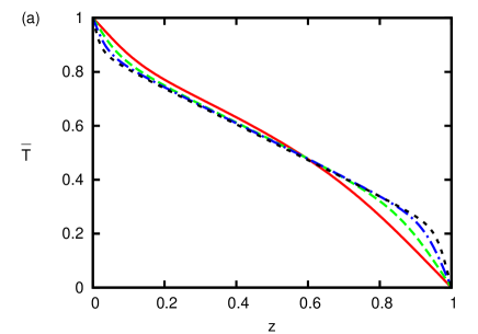
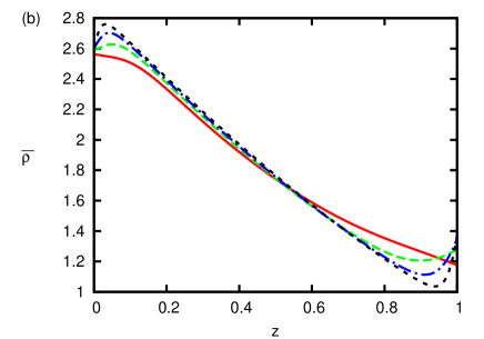
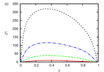
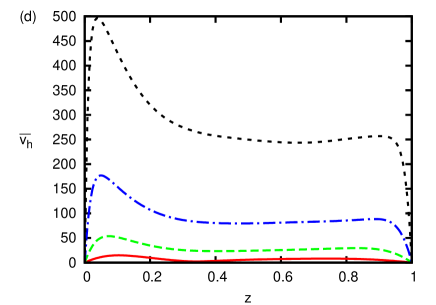
Figure 1: (Color online) Variations as a function of height $z$ of horizontal averages of temperature $T$ (top panel), density $\rho$ (second panel from the top), vertical velocity $v_{z}$ (third panel) and horizontal velocity (bottom panel). The overbars signal averages over time and horizontal planes. The different traces are for $\frac{\Delta T}{T_{o}}=\frac{d}{H_{o}}=3$ and the Rayleigh numbers $2\times 10^{4}$ (solid red line), $2\times 10^{5}$ (long dashed green line), $2\times 10^{6}$ (dot dashed blue line), $2\times 10^{7}$ (short dashed black line).

The well known Boussinesq approximation is recovered from equations (5-II) in the limit $d/H_{o}\rightarrow 0$ and $\Delta T/T_{o}\rightarrow 0$ Tritton (1988). In this limit, the sound speed goes to infinity. A purely explicit time step will be used in the numerical method below, so that simulations close to the Boussinesq limit become impractical. For this reason, and since the Boussinesq limit is an important reference case, a second system of equations was also implemented numerically:

$$\partial_{t}\rho+\nabla\cdot\bm{v}=0$$ (14)

$$\partial_{t}\bm{v}+(\bm{v}\cdot\nabla)\bm{v}=-c^{2}\nabla\rho+\mathrm{Pr}~{}\mathrm{Ra}~{}\theta{\bm{z}}+\mathrm{Pr}\nabla^{2}\bm{v}$$ (15)

$$\partial_{t}\theta+\bm{v}\cdot\nabla\theta-v_{z}=\nabla^{2}\theta$$ (16)

where $\theta$ is the deviation from the conductive profile, $T=1-z+\theta$. The sound speed $c$ appears as an independent variable. For small Mach numbers, the density fluctuations are small and the equation of continuity can be linearized to yield (14). The Boussinesq equations are recovered in the limit $c\rightarrow\infty$. In the simulations mentioned below using (14-16), the sound speed was adjusted such that the Mach number always stayed below 0.1. Note that simulations of weakly compressible convection as an approximation to Boussinesq convection have been undertaken before. For instance, simulations using the lattice Boltzmann method Lohse and Toschi (2003) implicitly do so.

Systems (5-II) and (14-16) have been simulated with a finite difference method implemented on graphic processing units using C for CUDA. The numerical method used centered finite differences of second order on a collocated grid except for the advection terms which used an upwind biased third order scheme. The time step was a third order Runge-Kutta method. The standard resolution was $256^{3}$. Lower resolution was sufficient at the smallest simulated $\mathrm{Ra}$. The validation of the code is described in the appendix.

III Results

III.1 Overview

A summary of the simulations is given in table 1. Apart from the control parameters, it lists the Nusselt number, defined as

$$\mathrm{Nu}=-\overline{\frac{dT}{dz}}$$ (17)

where the overbar denotes average over time and either top or bottom boundary. The kinetic energy density $E_{\mathrm{kin}}$ is given by

$$E_{\mathrm{kin}}=\frac{1}{V}\int\frac{1}{2}\rho\bm{v}^{2}dV$$ (18)

whereas the Peclet number $\mathrm{Pe}$ is computed from

$$\mathrm{Pe}=\sqrt{\frac{1}{V}\int\frac{1}{2}\bm{v}^{2}dV}$$ (19)

which is aptly called Peclet number because velocities are computed in units of $\kappa_{o}/d$. The average temperature deviation from the conductive profile at the center of the layer, $\bar{\theta}_{m}$, is also listed in table 1, together with the average density in the midplane, $\bar{\rho}_{m}$.

Fig. 1 shows vertical profiles of temperature, density, vertical velocity, and horizontal velocity $(v_{x}^{2}+v_{y}^{2})^{1/2}$ for different $\mathrm{Ra}$. Contrary to the Boussinesq case, these profiles are not symmetric about the midplane. The relation between the top and bottom regions of the layer will be discussed in section III.3. As $\mathrm{Ra}$ increases, an increasingly large interval develops in which the temperature gradient is approximately equal to the adiabatic gradient. The maximum of the vertical velocity is found below the midplane. Two local maxima show up in the profiles of horizontal velocity. The larger velocities are found near the bottom boundary. When both $d/H_{o}$ and $Ra$ are large, there is no local maximum of horizontal velocity near the top boundary and the horizontal velocity decreases monotonically with height. These cases result in blanks in the last column of table 1. Boundary layers also exist in the density profiles. The average density takes its maximum and minimum values, $\rho_{\mathrm{max}}$ and $\rho_{\mathrm{min}}$, near the bottom and top boundary, respectively. Both $\rho_{\mathrm{max}}$ and $\rho_{\mathrm{min}}$ are given in table 1, too. The ratio $\rho_{\mathrm{max}}/\rho_{\mathrm{min}}$ is generally less than is suggested by the values of $d/H_{o}$ and the initial conditions (13) because the statistically stationary, turbulent and well mixed state is nearly adiabatic, not conductive. A rough estimate of $\rho_{\mathrm{max}}/\rho_{\mathrm{min}}$ can be obtained from assuming that the adiabatic state extends throughout the layer, implying that the density takes its extremal values exactly on the boundaries. This leads to

$$\frac{\rho_{\mathrm{max}}}{\rho_{\mathrm{min}}}\approx\left(\frac{T_{m}+\frac{1}{2}\Delta T_{\mathrm{ad}}}{T_{m}-\frac{1}{2}\Delta T_{\mathrm{ad}}}\right)^{1/(\gamma-1)}$$ (20)

with $T_{m}=(\bar{\theta}_{m}+\frac{1}{2})\Delta T+T_{o}$, which is compatible with the numerical results.

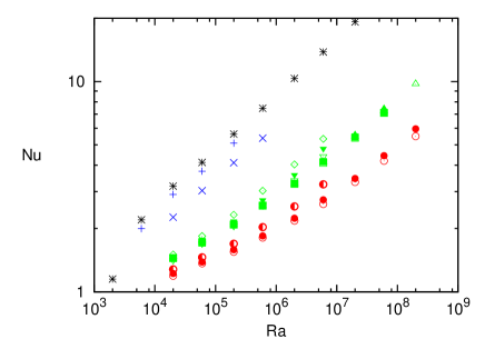
Figure 2: (Color online) Nusselt number $\mathrm{Nu}$ as a function of Rayleigh number $\mathrm{Ra}$ within the Boussinesq approximation (black stars), for $\Delta T_{\mathrm{ad}}/\Delta T=1/15$ (blue symbols) and $\Delta T/T_{o}=0.1$ (plus) and 1 (x), for $\Delta T_{\mathrm{ad}}/\Delta T=2/3$ (green symbols) and $\Delta T/T_{o}=0.1$ (empty squares), 0.3 (full squares), 1 (empty triangle up), 3 (full triangle up), 10 (empty triangle down), 30 (full triangle down) and 100 (empty diamonds) and for $\Delta T_{\mathrm{ad}}/\Delta T=4/5$ (red symbols) and $\Delta T/T_{o}=0.1$ (empty circles), 1 (full circles) and 10 (half filled circles). Data for the Boussinesq case do not appear in the subsequent figures.

III.2 Global Quantities

The most immediate task is of course to find predictions for the Nusselt number. A straightforward plot of $\mathrm{Nu}$ vs. $\mathrm{Ra}$ (fig. 2) shows that one does not obtain simple power laws for large $\Delta T_{\mathrm{ad}}/\Delta T$ and $d/H_{o}$. A finite adiabatic temperature gradient modifies the onset of convection. If one aims for a data reduction which collapses the different curves in fig. 2, one can account for the adiabatic temperature difference by defining a corrected Rayleigh number $\mathrm{Ra}_{*}$ by

$$\mathrm{Ra}_{*}=\frac{gd^{3}(\Delta T-\Delta T_{\mathrm{ad}})}{T_{o}\kappa_{o}\nu_{o}}=\mathrm{Ra}\left(1-(\gamma-1)\frac{d}{H_{o}}\frac{T_{o}}{\Delta T}\right).$$ (21)

A similar correction seems in order for $\mathrm{Nu}$. Since the adiabatic temperature gradient needs to be established before any convection can start, it is natural to subtract the heat conducted down the adiabat from both the actual heat transport and the conductive heat transport used for the normalization of the heat transport Massaguer and Zahn (1980):

$$\mathrm{Nu}_{*}=\frac{\mathrm{Nu}-\Delta T_{\mathrm{ad}}/\Delta T}{1-\Delta T_{\mathrm{ad}}/\Delta T}.$$ (22)

It is seen from fig. 3 that for $\mathrm{Ra}_{*}$ larger than roughly $10^{5}$, one finds approximately $(\mathrm{Nu}_{*}-1)\propto\mathrm{Ra}_{*}^{0.3}$, but the prefactors depend on the other control parameters in a non-trivial way. This is compatible with an argument exposed in Ref. Furukawa and Onuki, 2002, which states that $\mathrm{Ra}(\mathrm{Nu}-1)=f(\mathrm{Ra}_{*})$ with $f$ an a priori unknown function. The argument has to assume negligible viscous heating and small density variations, so that it is not expected to hold throughout the parameter range investigated here. Nonetheless, a best fit to the data yields $\mathrm{Ra}(\mathrm{Nu}-1)=\mathrm{Ra}_{*}^{1.3}/8.5$ which can be rearranged into the fitting function in fig. 3, $(\mathrm{Nu}_{*}-1)=\mathrm{Ra}_{*}^{0.3}/8.5$.

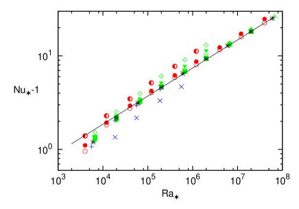
Figure 3: (Color online) $\mathrm{Nu}_{*}$ as a function of $\mathrm{Ra}_{*}$ with the same symbols as in fig. 2. The solid line indicates the power law $\mathrm{Nu}_{*}=\mathrm{Ra}_{*}^{0.3}/8.5$.

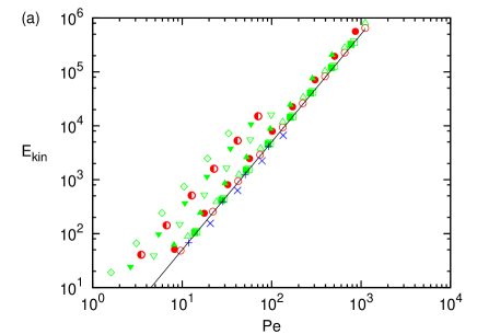
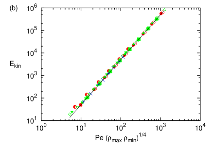
Figure 4: (Color online) The kinetic energy density $E_{\mathrm{kin}}$ as a function of $\mathrm{Pe}$ (top panel) and $\mathrm{Pe}(\rho_{\mathrm{max}}\rho_{\mathrm{min}})^{1/4}$ (bottom panel) with the same symbols as in fig. 2. The solid lines are given by $E_{\mathrm{kin}}=\frac{1}{2}\mathrm{Pe}^{2}$ (top panel) and $E_{\mathrm{kin}}=\frac{1}{2}\sqrt{\rho_{\mathrm{max}}\rho_{\mathrm{min}}}~{}\mathrm{Pe}^{2}$ (bottom panel).

It can also be useful to relate $\mathrm{Nu}$ to the kinetic energy or the Peclet number. It was noted in Ref. Schmitz and Tilgner, 2009 that $(\mathrm{Nu}-1)\propto\mathrm{Pe}^{2/3}$ in Boussinesq convection in computational volumes of large aspect ratio, which is equivalent to $(\mathrm{Nu}-1)\propto E_{\mathrm{kin}}^{1/3}$ in that case. In the present simulations, the relation between $E_{\mathrm{kin}}$ and $\mathrm{Pe}$ is already non-trivial (see fig. 4), because there is a factor representing an effective density between the two quantities. It turns out that the geometric mean of $\rho_{\mathrm{max}}$ and $\rho_{\mathrm{min}}$ is a suitable effective density to the extent that in fig. 4, all points for $\mathrm{Ra}_{*}(\rho_{\mathrm{max}}\rho_{\mathrm{min}})^{1/4}>100$ deviate by less than 30 % in $E_{\mathrm{kin}}$ from

$$E_{\mathrm{kin}}=\frac{1}{2}\sqrt{\rho_{\mathrm{max}}\rho_{\mathrm{min}}}~{}\mathrm{Pe}^{2}.$$ (23)

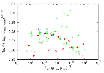
Figure 5: (Color online) $\mathrm{Nu}_{*}-1$ as a function of $E_{\mathrm{kin}}(\rho_{\mathrm{max}}\rho_{\mathrm{min}})^{1/2}$, compensated for the power law in Eq. (24), with the same symbols as in fig. 2.

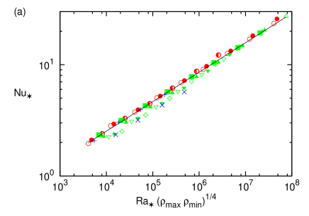
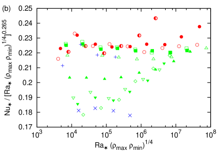
Figure 6: (Color online) $\mathrm{Nu}_{*}$ as a function of $\mathrm{Ra}_{*}(\rho_{\mathrm{max}}\rho_{\mathrm{min}})^{1/4}$, on a double logaritmic scale in the top panel and compensated for the power law in Eq. (25) in the bottom panel, with the same symbols as in fig. 2.

This geometric mean becomes again important when looking for a relation between $\mathrm{Nu}_{*}-1$ and $E_{\mathrm{kin}}$. A good fit to the data is obtained from

$$\mathrm{Nu}_{*}-1=\frac{2}{7}(E_{\mathrm{kin}}\sqrt{\rho_{\mathrm{max}}\rho_{\mathrm{min}}})^{1/3}$$ (24)

(see fig. 5) which reduces of course to the previously known scaling Schmitz and Tilgner (2009, 2010) for $\rho_{\mathrm{max}}=\rho_{\mathrm{min}}$ and $\Delta T_{\mathrm{ad}}/\Delta T=0$.

Having established the relevance of the product $\rho_{\mathrm{max}}\rho_{\mathrm{min}}$, it is tempting to introduce it into fits of $\mathrm{Nu}_{*}$ vs. $\mathrm{Ra}_{*}$. A reasonable fit is shown in fig. 6 to be

$$\mathrm{Nu}_{*}=0.22\left(\mathrm{Ra}_{*}(\rho_{\mathrm{max}}\rho_{\mathrm{min}})^{1/4}\right)^{0.265},$$ (25)

which is an improvement compared with fig. 3 especially for $\mathrm{Ra}_{*}(\rho_{\mathrm{max}}\rho_{\mathrm{min}})^{1/4}>10^{6}$.

III.3 Boundary Layers

Previous studies have quantified the asymmetry between top and bottom in non-Boussinesq convection with the help of the midplane temperature Wu and Libchaber (1991); Ahlers et al. (2007). In most of the present simulations, the midplane temperature deviates by less than $0.05~{}\Delta T$ from its value in the conductive state (see table 1). Such a small deviation is difficult to determine accurately and requires long time integrations, so that this section will not consider $\bar{\theta}_{m}$ any further, apart from noting that $\bar{\theta}_{m}$ is negative for small $\Delta T_{\mathrm{ad}}/\Delta T$ (in agreement with Ref. Ahlers et al., 2007) but becomes positive for $\Delta T_{\mathrm{ad}}/\Delta T$ large enough.

A relation between temperature boundary layers deduced from experimental data by Wu and Libchaber Wu and Libchaber (1991) is based on a temperature scale computed from quantities local to each boundary layer. In many of the simulations presented here, the boundary layers are still quite thick and there is significant variation of for example thermal diffusivity across them, so that the results of Wu and Libchaber cannot be tested in a meaningful way.

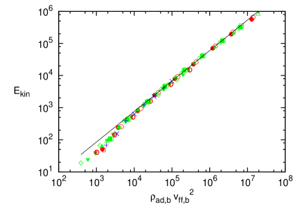
Figure 7: (Color online) $E_{\mathrm{kin}}$ as a function of $\rho_{\mathrm{ad,b}}v_{\mathrm{ff,b}}^{2}$ with the same symbols as in fig. 2. The solid line indicates the power law $E_{\mathrm{kin}}=0.12~{}(\rho_{\mathrm{ad,b}}v_{\mathrm{ff,b}}^{2})^{0.95}$.

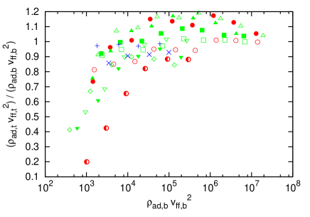
Figure 8: (Color online) $(\rho_{\mathrm{ad,t}}v_{\mathrm{ff,t}}^{2})/(\rho_{\mathrm{ad,b}}v_{\mathrm{ff,b}}^{2})$ as a function of $\rho_{\mathrm{ad,b}}v_{\mathrm{ff,b}}^{2}$ with the same symbols as in fig. 2.

In the following, overbars denote averages over time and horizontal planes, and the indices b and t indicate top and bottom boundaries. For example, $\bar{\rho}_{t}$ is the average density at the top boundary. It is in general different from $\rho_{o}$, which is the density at the top boundary in the initial conductive state given by Eq. (13).

This subsection will present two relations between the top and bottom regions of the convection layer involving the free fall velocity. In order to compute a free fall velocity, we define $T_{\mathrm{ad,t}}$ and $T_{\mathrm{ad,b}}$ as the (dimensional) temperatures the gas would have at the top and bottom boundaries if the adiabatic temperature profile extended throughout the entire layer:

$$T_{\mathrm{ad,t}}=T_{m}-\frac{1}{2}\Delta T_{\mathrm{ad}}~{}~{}~{},~{}~{}~{}T_{\mathrm{ad,b}}=T_{m}+\frac{1}{2}\Delta T_{\mathrm{ad}}$$ (26)

with $T_{m}=(\bar{\theta}_{m}+\frac{1}{2})\Delta T+T_{o}$. Under the same assumption, the densities at the two boundaries, $\rho_{\mathrm{ad,t}}$ and $\rho_{\mathrm{ad,b}}$, are given by

$$\rho_{\mathrm{ad,t}}=\bar{\rho}_{m}\left(\frac{T_{\mathrm{ad,t}}}{T_{m}}\right)^{1/(\gamma-1)}~{}~{}~{},~{}~{}~{}\rho_{\mathrm{ad,b}}=\bar{\rho}_{m}\left(\frac{T_{\mathrm{ad,b}}}{T_{m}}\right)^{1/(\gamma-1)}.$$ (27)

Consider now a parcel of gas near the top boundary. It has on average the density $\bar{\rho}_{t}$. The density difference with the adiabatic profile, $\bar{\rho}_{t}-\rho_{\mathrm{ad,t}}$, accelerates the parcel through the volume. The free fall velocity is estimated from a balance between the advection and buoyancy terms, which reads in the non-dimensional variables used here $|\rho(\bm{v}\cdot\nabla)\bm{v}|\sim\Delta\rho gd(d/\kappa_{o})^{2}$, where $\Delta\rho$ is the density difference of the moving parcel with the adiabatically stratified background. The pressure variation experienced by the falling parcel compresses the parcel by the same factor as the surrounding gas (assuming the parcel does not exchange heat with its surroundings), so that $\Delta\rho/\rho$ remains constant during the entire journey through the adiabatically stratified layer. It follows that $\Delta\rho/\rho$ keeps its initial value of $(\bar{\rho}_{t}-\rho_{\mathrm{ad,t}})/\bar{\rho}_{t}$, and that the square of the non-dimensional free fall velocity of the parcel arriving at the bottom (which is expressed in units of ($\kappa_{o}/d)^{2}$) is $\frac{\bar{\rho}_{t}-\rho_{\mathrm{ad,t}}}{\bar{\rho}_{t}}gd\left(\frac{d}{\kappa_{o}}\right)^{2}$. A similar expression is derived if we start the argument from the bottom boundary, so that we obtain two velocities, $v_{\mathrm{ff,t}}$ and $v_{\mathrm{ff,b}}$ according to the formula

$$v_{\mathrm{ff,t}} = \left(\frac{\bar{\rho}_{t}-\rho_{\mathrm{ad,t}}}{\bar{\rho}_{t}}\mathrm{Pr}~{}\mathrm{Ra}\frac{T_{o}}{\Delta T}\right)^{1/2},$$

$$v_{\mathrm{ff,b}} = \left(\frac{\rho_{\mathrm{ad,b}}-\bar{\rho}_{b}}{\bar{\rho}_{b}}\mathrm{Pr}~{}\mathrm{Ra}\frac{T_{o}}{\Delta T}\right)^{1/2}.$$ (28)

Fig. 7 verifies that one obtains with Eq. (28) a velocity representative of the convective velocity. The figure shows $E_{\mathrm{kin}}$ as a function of the energy density computed from the bottom free fall velocity, $\rho_{\mathrm{ad,b}}v_{\mathrm{ff,b}}^{2}$. When this velocity is small, the Reynolds number of the flow is too small for friction to be negligible and the free fall velocity is a poor estimate of the true velocity. For large velocities, there is a unique relation between $E_{\mathrm{kin}}$ and $\rho_{\mathrm{ad,b}}v_{\mathrm{ff,b}}^{2}$ independent of any other parameters.

It is now expected that one obtains the same graph if one uses the kinetic energy density computed at the top boundary, or equivalently, that $\rho_{\mathrm{ad,t}}v_{\mathrm{ff,t}}^{2}=\rho_{\mathrm{ad,b}}v_{\mathrm{ff,b}}^{2}$. Fig. 8 demonstrates that this is the case to within $\pm 20\%$ for sufficiently large velocities and over three decades in $\rho_{\mathrm{ad,b}}v_{\mathrm{ff,b}}^{2}$. The equality of the two energy densities is the first important connection between the top and bottom boundaries.

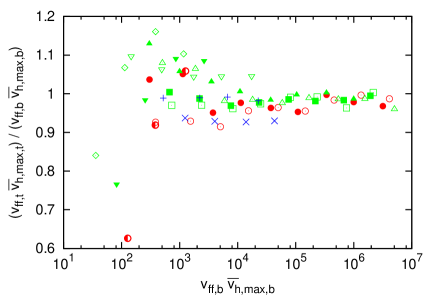
Figure 9: (Color online) $(v_{\mathrm{ff,t}}{\bar{v}}_{\mathrm{h,max,t}})/(v_{\mathrm{ff,b}}{\bar{v}}_{\mathrm{h,max,b}})$ as a function of $v_{\mathrm{ff,b}}{\bar{v}}_{\mathrm{h,max,b}}$ with the same symbols as in fig. 2.

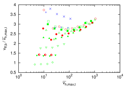
Figure 10: (Color online) $v_{\mathrm{ff,b}}/{\bar{v}}_{\mathrm{h,max,t}}$ as a function of ${\bar{v}}_{\mathrm{h,max,t}}$ with the same symbols as in fig. 2.

The second relation, shown in fig. 9, involves the local maxima of horizontal velocity near the top and bottom boundaries visible in the bottom panel of fig. 1. These maximum velocities, ${\bar{v}}_{\mathrm{h,max,t}}$ and ${\bar{v}}_{\mathrm{h,max,b}}$, are listed in table 1. According to fig. 9, they obey for sufficiently large velocities:

$$v_{\mathrm{ff,t}}{\bar{v}}_{\mathrm{h,max,t}}=v_{\mathrm{ff,b}}{\bar{v}}_{\mathrm{h,max,b}}.$$ (29)

${\bar{v}}_{\mathrm{h,max,b}}$ is a free fall velocity computed from quantities evaluated at the the bottom boundary, but it estimates the velocity of plumes arriving at the top boundary. The typical velocity of the flow out of the arriving plumes is the maximum average horizontal velocity, so that we expect ${\bar{v}}_{\mathrm{h,max,t}}\propto v_{\mathrm{ff,b}}$, and similarly ${\bar{v}}_{\mathrm{h,max,b}}\propto v_{\mathrm{ff,t}}$. The prefactors depend on the size of the incoming plumes relative to the thickness of the layer in which the outflow occurs. Fig. 10 shows that ${\bar{v}}_{\mathrm{h,max,t}}\propto v_{\mathrm{ff,b}}$ approximately holds and that the prefactor indeed depends on $d/H_{o}$ and $\Delta T/T_{o}$. The two proportionalities combine to $v_{\mathrm{ff,t}}{\bar{v}}_{\mathrm{h,max,t}}\propto v_{\mathrm{ff,b}}{\bar{v}}_{\mathrm{h,max,b}}$. It is remarkable that this combined relation is obeyed more accurately than the two separate proportionalities, and that the proportionality factor in the combined relation approaches 1 at high Rayleigh numbers as shown in fig. 9.

IV Conclusion

There are many ways how to depart from the Boussinesq approximation Wu and Libchaber (1991); Kogan et al. (1999); Burnishev et al. (2010); Ahlers et al. (2007) and it is not known at present whether there is anything universal about convection in general. The Prandtl number is a constant in a real gas and the Nusselt number depends only on the Rayleigh number in the Boussinesq limit. Away from that limit, several more control parameters determine the Nusselt number and it is a challenge to find a suitable data reduction such that the $Nu(Ra)$ dependences found for various density stratifications collapse on a single master curve, which then must contain the Boussinesq limit. It has been shown in the present paper that a good, if imperfect, data collapse is obtained if one introduces into the scaling laws an effective density given by the geometric mean of the maximum and minimum densities in the convecting layer. There is no theory underpinning the relevance of the geometric mean. It seems likely that the geometric mean will be of no help in some other cases of non-Boussinesq convection, for example in liquids.

On the other hand, the importance of free fall velocities has been recognized since long, and it has been shown here that two different estimates of free fall velocities, based on quantities pertaining either to the top or the bottom boundary, are related at high Rayleigh numbers by the requirement that the kinetic energy densities computed from the two velocities must be equal. The free fall velocities are also connected to the total kinetic energy of the flow and the maxima of the horizontal velocity profile. It will be worthwhile to check these relations in other forms of convection.

*

Appendix A

This appendix describes a few tests that have been performed in order to validate the numerical code. Direct validation of the code is problematic because published simulations of compressible convection either focus on flow structures Toomre et al. (1990); Porter and Woodward (2000) and are not useful as a benchmark, or are too close to the Boussinesq limit to offer a stringent test Robinson and Chan (2004). A different route had therefore to be taken.

First, the code simulating (14-16) could be validated against a completely independent spectral method Hartlep et al. (2003). This already verified most terms occurring in (5-II). For example, the spectral code calculates for a plane layer with no slip boundaries in $z$, periodic boundary conditions in $x$ and $y$ with $l_{x}=l_{y}=2d$, and $\mathrm{Pr}=0.7$ and $\mathrm{Ra}=1.6\times 10^{4}$ that $E_{\mathrm{kin}}=360$ and $\mathrm{Nu}=3.01$. If started from the initial conditions $\bm{v}=0$, $\theta=\sin(\pi z)\cos(2\pi y)\cos(2\pi x)$ at $t=0$, the system (14-16) needs to be integrated beyond $t=10$ to find the final state. The new code with appropriately adapted boundary conditions yields $E_{\mathrm{kin}}=351$ and $\mathrm{Nu}=2.96$ for 32 points along $z$ and $64^{2}$ grid points in the $x,y-$plane. At twice that resolution in each coordinate, the result is $E_{\mathrm{kin}}=357$ and $\mathrm{Nu}=2.99$. The parameter $c^{2}$ in Eq. (15) was set to $10^{5}$ so that the Mach number is below $8.5\times 10^{-2}$.

In a next step, the code implementing (5-II) was used to simulate the propagation of sound waves. For this purpose, the term $-\hat{\bm{z}}\mathrm{Pr}~{}\mathrm{Ra}\frac{T_{o}}{\Delta T}$ was removed from Eq. (II). The remaining equations, if linearized and neglecting dissipation, can be manipulated into

$$\partial_{t}^{2}\bm{v}=\frac{T_{o}}{\Delta T}\frac{H_{o}}{d}\mathrm{Pr}~{}\mathrm{Ra}~{}\nabla(\nabla\cdot\bm{v}).$$

This equation allows some simple analytical solutions. For example, there are the eigenmodes depending only on $z$. The first of those eigenmodes for boundary conditions imposing zero heat flux at the top and bottom boundaries is of the form $v_{z}\propto\sin(\pi z)\cos(\omega t)$. This standing wave has a period of $\tau=2\pi/\omega=2(\frac{T_{o}}{\Delta T}\frac{H_{o}}{d}\mathrm{Pr}~{}\mathrm{Ra})^{-1/2}$. For $\frac{\Delta T}{T_{o}}=0.1$, $\frac{d}{H_{o}}=0.01$, $\mathrm{Pr}=0.7$ and $\mathrm{Ra}=2\times 10^{4}$, this predicts $\tau=5.345\times 10^{-4}$. With a resolution of 64 grid points along $z$, the numerical result is $\tau=5.343\times 10^{-4}$. One can similarly simulate sound waves propagating in different directions. This is a test for all terms involving $\nabla\cdot\bm{v}$. The fact that simulations of convection at high $\mathrm{Ra}$ yield a temperature gradient in the bulk close to the adiabatic gradient may also be regarded as a test of the terms involving $\nabla\cdot\bm{v}$.

The dissipation rate of the standing wave of the previous paragraph can be used to test the dissipative term. A more complete test is provided by the energy budget which also tests the viscous heating term in the temperature equation. If one takes the scalar product of Eq. (II) with $\bm{v}$ and integrates Eqs. (II) and (II), multiplied by $\rho$, over all space, one deduces from Eqs. (5-II) that the time derivative of kinetic plus internal energy is given by

$$\frac{d}{dt}\int\left[\frac{1}{2}\rho\bm{v}^{2}+\mathrm{Ra}~{}\mathrm{Pr}~{}\frac{H_{o}}{d}\frac{1}{\gamma}\frac{\rho}{\gamma-1}(T+\frac{T_{o}}{\Delta T})\right]dV=G+V_{1}+V_{2}$$

with

$$G = -\mathrm{Pr}~{}\mathrm{Ra}\frac{T_{o}}{\Delta T}\int\rho v_{z}dV,$$

$$V_{1} = \mathrm{Pr}\int v_{i}[\nabla^{2}v_{i}+\frac{1}{3}\partial_{i}(\nabla\cdot\bm{v})]dV,$$

$$V_{2} = \mathrm{Pr}\int 2[e_{ij}-\frac{1}{3}\nabla\cdot\bm{v}\delta_{ij}]^{2}dV.$$

$G$ is the work done by gravity, $V_{1}$ the dissipated kinetic energy and $V_{2}$ the heat generated through viscous dissipation. If we denote time averages by angular brackets, we must find in a statistically stationary state that $\langle G\rangle=0$ and $\langle V_{1}\rangle+\langle V_{2}\rangle=0$. Since $V_{1}$ and $V_{2}$ have different forms and must be programmed differently, the energy budget provides a good test for their correctness. For the case $\frac{\Delta T}{T_{o}}=\frac{d}{H_{o}}=1$ and $\mathrm{Ra}=6\times 10^{4}$ included in table 1, the simulations yield $|\langle G\rangle/\langle V_{1}\rangle|=3.3\times 10^{-3}$ and $|\langle V_{1}+V_{2}\rangle/\langle V_{1}\rangle|=7.6\%$ at a resolution of $64^{3}$ grid points, and $|\langle G\rangle/\langle V_{1}\rangle|=4.2\times 10^{-4}$ and $|\langle V_{1}+V_{2}\rangle/\langle V_{1}\rangle|=4\%$ at a resolution of $128^{3}$ grid points. The formulae for $V_{1}$ and $V_{2}$ taken together contain integrals of 18 derivatives, 6 of which are squared, so that the typical error on each derivative is about $0.1\%$. The volume integrals have been computed by adding the integrands at each grid point, multiplied by the volume of the cell surrounding each grid point. This method of integration is of first order for general integrands Press et al. (1986), which explains why the error in $|\langle V_{1}+V_{2}\rangle/\langle V_{1}\rangle|$ is only halved when doubling the resolution.

$\frac{\Delta T}{T_{o}}$	$\frac{d}{H_{o}}$	$\mathrm{Ra}$	$\mathrm{Nu}$	$E_{\mathrm{kin}}$	$\mathrm{Pe}$	$100~{}\bar{\theta}_{m}$	$\bar{\rho}_{m}$	$\rho_{\mathrm{max}}$	$\rho_{\mathrm{min}}$	${\bar{v}}_{\mathrm{h,max,b}}$	${\bar{v}}_{\mathrm{h,max,t}}$
0.1	0.12	2$\times 10^{4}$	1.19	48.3	9.59	0.09	1.05	1.10	1.00	10.3	10
0.1	0.12	6$\times 10^{4}$	1.37	256	22.1	0.14	1.05	1.10	1.00	24.2	23
0.1	0.12	2$\times 10^{5}$	1.55	941	42.3	0.19	1.05	1.10	1.00	43.5	40.4
0.1	0.12	6$\times 10^{5}$	1.81	2.9$\times 10^{3}$	74.3	0.23	1.05	1.10	1.00	77.9	72.1
0.1	0.12	2$\times 10^{6}$	2.18	9.32$\times 10^{3}$	133	0.21	1.05	1.10	1.00	138	129
0.1	0.12	6$\times 10^{6}$	2.61	2.62$\times 10^{4}$	223	0.21	1.05	1.10	1.00	234	218
0.1	0.12	2$\times 10^{7}$	3.32	8.24$\times 10^{4}$	396	0.23	1.05	1.10	1.00	410	379
0.1	0.12	6$\times 10^{7}$	4.20	2.26$\times 10^{5}$	656	0.25	1.05	1.10	1.00	688	645
0.1	0.12	2$\times 10^{8}$	5.49	6.52$\times 10^{5}$	1.11$\times 10^{3}$	0.17	1.05	1.11	1.00	1.16$\times 10^{3}$	1.08$\times 10^{3}$
1	1.2	2$\times 10^{4}$	1.22	50.8	8.2	1.67	1.49	2.01	1.02	11.6	9.38
1	1.2	6$\times 10^{4}$	1.39	239	17.7	1.96	1.48	2.02	1.04	26.9	19.3
1	1.2	2$\times 10^{5}$	1.59	808	32.4	2.09	1.49	2.02	1.04	48.9	31
1	1.2	6$\times 10^{5}$	1.84	2.46$\times 10^{3}$	56.6	2.19	1.48	2.02	1.05	87.7	53.4
1	1.2	2$\times 10^{6}$	2.24	7.9$\times 10^{3}$	102	2.05	1.49	2.03	1.04	157	94.6
1	1.2	6$\times 10^{6}$	2.74	2.25$\times 10^{4}$	172	1.88	1.49	2.04	1.03	261	158
1	1.2	2$\times 10^{7}$	3.46	7.08$\times 10^{4}$	305	1.93	1.49	2.05	1.02	452	278
1	1.2	6$\times 10^{7}$	4.44	1.94$\times 10^{5}$	507	1.74	1.49	2.06	1.00	753	463
1	1.2	2$\times 10^{8}$	5.96	5.62$\times 10^{5}$	863	1.46	1.49	2.07	0.99	1.28$\times 10^{3}$	805
10	12	2$\times 10^{4}$	1.28	40.6	3.49	4.52	5.71	11.05	1.52	13.7	6.55
10	12	6$\times 10^{4}$	1.46	143	6.71	4.08	5.69	11.07	1.72	23.9	11.3
10	12	2$\times 10^{5}$	1.69	511	12.8	4.22	5.67	11.09	1.96	45.2	19.9
10	12	6$\times 10^{5}$	2.03	1.6$\times 10^{3}$	22.7	4.26	5.67	11.13	2.18	80.6
10	12	2$\times 10^{6}$	2.55	5.3$\times 10^{3}$	41.7	3.97	5.68	11.22	2.13	142
10	12	6$\times 10^{6}$	3.24	1.51$\times 10^{4}$	70.8	3.66	5.69	11.31	1.99	234
0.1	0.1	2$\times 10^{4}$	1.45	108	14.5	0.11	1.03	1.07	1.00	15.5	15
0.1	0.1	6$\times 10^{4}$	1.72	442	29.3	0.19	1.03	1.07	1.00	29.7	28.2
0.1	0.1	2$\times 10^{5}$	2.09	1.56$\times 10^{3}$	54.9	0.22	1.03	1.07	1.00	55.8	52.6
0.1	0.1	6$\times 10^{5}$	2.57	4.75$\times 10^{3}$	95.8	0.15	1.03	1.07	1.00	97.8	92.2
0.1	0.1	2$\times 10^{6}$	3.27	1.5$\times 10^{4}$	170	0.43	1.03	1.07	0.99	177	165
0.1	0.1	6$\times 10^{6}$	4.11	4.23$\times 10^{4}$	286	0.39	1.03	1.07	0.99	294	277
0.1	0.1	2$\times 10^{7}$	5.41	1.26$\times 10^{5}$	494	0.38	1.03	1.08	0.99	517	472
0.1	0.1	6$\times 10^{7}$	7.09	3.54$\times 10^{5}$	828	0.27	1.03	1.08	0.99	858	821
0.3	0.3	2$\times 10^{4}$	1.45	105	13.8	0.80	1.10	1.19	1.00	15.6	14.3
0.3	0.3	6$\times 10^{4}$	1.72	422	27.7	1.00	1.10	1.20	1.01	30.3	26.3
0.3	0.3	2$\times 10^{5}$	2.09	1.49$\times 10^{3}$	52	0.98	1.10	1.20	1.00	57.7	49
0.3	0.3	6$\times 10^{5}$	2.58	4.57$\times 10^{3}$	91	1.07	1.10	1.21	0.99	103	85.9
0.3	0.3	2$\times 10^{6}$	3.28	1.44$\times 10^{4}$	162	1.20	1.10	1.21	0.99	183	152
0.3	0.3	6$\times 10^{6}$	4.16	4.06$\times 10^{4}$	271	1.12	1.10	1.22	0.98	305	253
0.3	0.3	2$\times 10^{7}$	5.44	1.2$\times 10^{5}$	467	0.93	1.10	1.22	0.98	510	431
0.3	0.3	6$\times 10^{7}$	7.10	3.24$\times 10^{5}$	768	0.89	1.10	1.22	0.97	844	724
1	1	2$\times 10^{4}$	1.44	88.4	11.6	2.38	1.29	1.61	1.04	15.2	12.3
1	1	6$\times 10^{4}$	1.74	389	24.2	2.45	1.29	1.62	1.05	33.9	25
1	1	2$\times 10^{5}$	2.10	1.24$\times 10^{3}$	43.2	2.68	1.29	1.63	1.03	58.8	39.6
1	1	6$\times 10^{5}$	2.57	3.78$\times 10^{3}$	75.4	2.80	1.29	1.65	1.01	105	68.6
1	1	2$\times 10^{6}$	3.26	1.18$\times 10^{4}$	133	2.74	1.29	1.66	1.00	185	120
1	1	6$\times 10^{6}$	4.14	3.38$\times 10^{4}$	226	2.76	1.29	1.68	0.98	311	202
1	1	2$\times 10^{7}$	5.48	1.03$\times 10^{5}$	396	2.52	1.29	1.69	0.96	537	354
1	1	6$\times 10^{7}$	7.23	2.82$\times 10^{5}$	655	2.21	1.29	1.70	0.95	875	589
1	1	2$\times 10^{8}$	9.75	8.09$\times 10^{5}$	1.11$\times 10^{3}$	1.81	1.30	1.71	0.94	1.52$\times 10^{3}$	1.03$\times 10^{3}$

Table 1: Summary of results. Listed are the control parameters $\frac{\Delta T}{T_{o}}$, $\frac{d}{H_{o}}$, and $\mathrm{Ra}$ together with $\mathrm{Nu}$, $E_{\mathrm{kin}}$, $\mathrm{Pe}$, $\bar{\theta}_{m}$ multiplied by 100, $\bar{\rho}_{m}$, $\rho_{\mathrm{max}}$, $\rho_{\mathrm{min}}$, ${\bar{v}}_{\mathrm{h,max,b}}$, and ${\bar{v}}_{\mathrm{h,max,t}}$ (see text for definitions). The table consists of three sections (corresponding to the color code of the figures in the online version) with different $\Delta T_{\mathrm{ad}}/\Delta T$, which is 4/5, 2/3 or 1/15 in going from the top to the end of the table. An entry is missing for ${\bar{v}}_{\mathrm{h,max,t}}$ if the profile of horizontal velocity has no maximum near the top boundary.

$\frac{\Delta T}{T_{o}}$	$\frac{d}{H_{o}}$	$\mathrm{Ra}$	$\mathrm{Nu}$	$E_{\mathrm{kin}}$	$\mathrm{Pe}$	$100~{}\bar{\theta}_{m}$	$\bar{\rho}_{m}$	$\rho_{\mathrm{max}}$	$\rho_{\mathrm{min}}$	${\bar{v}}_{\mathrm{h,max,b}}$	${\bar{v}}_{\mathrm{h,max,t}}$
3	3	2$\times 10^{4}$	1.42	61.6	8.11	4.08	1.75	2.56	1.17	13.5	9.66
3	3	6$\times 10^{4}$	1.68	241	15.9	4.36	1.75	2.58	1.23	27	16.3
3	3	2$\times 10^{5}$	2.05	853	30	4.51	1.75	2.63	1.21	53.6	29.4
3	3	6$\times 10^{5}$	2.52	2.59$\times 10^{3}$	52.5	4.31	1.76	2.66	1.16	94.9	49.9
3	3	2$\times 10^{6}$	3.25	8.8$\times 10^{3}$	96.7	4.29	1.76	2.70	1.11	177	88.4
3	3	6$\times 10^{6}$	4.16	2.44$\times 10^{4}$	162	4.15	1.77	2.73	1.07	283	144
3	3	2$\times 10^{7}$	5.59	7.57$\times 10^{4}$	286	3.83	1.77	2.76	1.04	496	257
3	3	6$\times 10^{7}$	7.45	2.06$\times 10^{5}$	473	3.32	1.77	2.79	1.00	822	431
10	10	2$\times 10^{4}$	1.42	39.1	4.81	5.33	3.04	5.00	1.60	11.3	7.37
10	10	6$\times 10^{4}$	1.70	149	9.39	5.09	3.04	5.05	1.84	22.1	12.3
10	10	2$\times 10^{5}$	2.06	529	17.7	5.58	3.02	5.14	1.83	45.2	21.6
10	10	6$\times 10^{5}$	2.58	1.65$\times 10^{3}$	31.3	5.41	3.03	5.22	1.73	78.3	35.6
10	10	2$\times 10^{6}$	3.38	5.54$\times 10^{3}$	57.7	5.09	3.04	5.31	1.61	141	62.6
10	10	6$\times 10^{6}$	4.40	1.61$\times 10^{4}$	98.8	4.82	3.05	5.38	1.52	237
30	30	2$\times 10^{4}$	1.46	24.5	2.64	7.27	5.78	9.91	2.56	11.2	5.29
30	30	6$\times 10^{4}$	1.77	97.6	5.46	5.66	5.74	10.03	3.32	19.5	9.58
30	30	2$\times 10^{5}$	2.17	368	10.7	5.57	5.69	10.20	3.20	37.1	17.1
30	30	6$\times 10^{5}$	2.73	1.14$\times 10^{3}$	18.9	5.37	5.70	10.36	2.99	65.8	28.7
30	30	2$\times 10^{6}$	3.60	3.79$\times 10^{3}$	34.6	5.22	5.72	10.53	2.76	118
30	30	6$\times 10^{6}$	4.80	1.07$\times 10^{4}$	58.8	4.68	5.75	10.70	2.55	193
100	100	2$\times 10^{4}$	1.50	19	1.6	6.86	12.29	21.72	5.17	8.92	4.4
100	100	6$\times 10^{4}$	1.84	66.3	3.08	5.85	12.26	22.02	6.96	15.9	7.66
100	100	2$\times 10^{5}$	2.33	242	5.95	5.56	12.21	22.38	6.57	29.8	13.7
100	100	6$\times 10^{5}$	3.02	746	10.5	5.36	12.24	22.73	6.04	52.1	22
100	100	2$\times 10^{6}$	4.03	2.47$\times 10^{3}$	19.2	4.92	12.28	23.14	5.53	92.5
100	100	6$\times 10^{6}$	5.34	7.25$\times 10^{3}$	33.1	4.41	12.29	23.53	5.11	161
0.1	0.01	6$\times 10^{3}$	2.00	67.5	11.9	-0.90	0.96	0.96	0.96	12	12
0.1	0.01	2$\times 10^{4}$	2.90	392	28.6	-0.44	0.96	0.96	0.96	28.2	28.1
0.1	0.01	6$\times 10^{4}$	3.75	1.23$\times 10^{3}$	50.6	-0.73	0.96	0.96	0.96	48.3	48.4
0.1	0.01	2$\times 10^{5}$	5.10	4.14$\times 10^{3}$	92.7	-0.40	0.96	0.96	0.96	90.3	88.9
1	0.1	2$\times 10^{4}$	2.26	155	20.6	-1.67	0.73	0.74	0.72	18.3	17.9
1	0.1	6$\times 10^{4}$	3.03	632	41.6	-1.32	0.73	0.74	0.72	34.8	32.9
1	0.1	2$\times 10^{5}$	4.11	2.24$\times 10^{3}$	78.2	-1.47	0.73	0.74	0.72	66.3	62.1
1	0.1	6$\times 10^{5}$	5.38	6.65$\times 10^{3}$	135	-1.26	0.73	0.74	0.72	119	111

Table 2: Table 1 continued.

References

- Ahlers et al. (2009) G. Ahlers, S. Grossmann, and D. Lohse, Rev. Mod. Phys. 81, 503 (2009).
- Tritton (1988) D. Tritton, Physical Fluid Dynamics (Oxford University Press, Oxford, 1988).
- Wu and Libchaber (1991) X.-Z. Wu and A. Libchaber, Phys. Rev. A 43, 2833 (1991).
- Ahlers et al. (2007) G. Ahlers, F. Fontenele Araujo, D. Funfschilling, S. Grossmann, and D. Lohse, Phys. Rev. Lett. 98, 054501 (2007).
- Ashkenazi and Steinberg (1999) S. Ashkenazi and V. Steinberg, Phys. Rev. Lett. 83, 3641 (1999).
- Kogan et al. (1999) A. Kogan, D. Murphy, and H. Meyer, Phys. Rev. Lett. 82, 4635 (1999).
- Burnishev et al. (2010) Y. Burnishev, E. Segre, and V. Steinberg, Phys. Fluids 22, 035108 (2010).
- Chavanne et al. (1997) X. Chavanne, F. Chilla, B. Castaing, B. Hébral, B. Chabaud, and J. Chaussy, Phys. Rev. Lett. 79, 3684 (1997).
- Niemela et al. (2000) J. J. Niemela, L. Skrbek, K. R. Sreenivasan, and R. J. Donnelly, Nature 404, 837 (2000).
- Salby (1996) M. Salby, Fundamentals of Atmospheric Physics (Academic Press, San Diego, 1996).
- Toomre et al. (1990) J. Toomre, N. Brummell, F. Cattaneo, and N. Hurlburt, Computer Physics Communications 59, 105 (1990).
- Lohse and Toschi (2003) D. Lohse and F. Toschi, Phys. Rev. Lett. 90, 034502 (2003).
- Massaguer and Zahn (1980) J. Massaguer and J.-P. Zahn, Astron. Astrophys. 87, 315 (1980).
- Furukawa and Onuki (2002) A. Furukawa and A. Onuki, Phys. Rev. E 66, 016302 (2002).
- Schmitz and Tilgner (2009) S. Schmitz and A. Tilgner, Phys. Rev. E 80, 015305(R) (2009).
- Schmitz and Tilgner (2010) S. Schmitz and A. Tilgner, Geophys. Astrophys. Fluid Dyn. 104, 481 (2010).
- Porter and Woodward (2000) D. Porter and P. Woodward, Astrophys. J. Suppl. 127, 159 (2000).
- Robinson and Chan (2004) F. Robinson and K. Chan, Phys. Fluids 16, 1321 (2004).
- Hartlep et al. (2003) T. Hartlep, A. Tilgner, and F. H. Busse, Phys. Rev. Lett. 91, 064501 (2003).
- Press et al. (1986) W. Press, S. Teukolsky, W. Vetterling, and B. Flannery, Numerical Recipes (Cambridge University Press, Cambridge, 1986).