Fill-ins of nonnegative scalar curvature, static metrics, and quasi-local mass

Abstract.

Consider a triple of “Bartnik data” $(\Sigma,\gamma,H)$, where $\Sigma$ is a topological 2-sphere with Riemannian metric $\gamma$ and positive function $H$. We view Bartnik data as a boundary condition for the problem of finding a compact Riemannian 3-manifold $(\Omega,g)$ of nonnegative scalar curvature whose boundary is isometric to $(\Sigma,\gamma)$ with mean curvature $H$. Considering the perturbed data $(\Sigma,\gamma,\lambda H)$ for a positive real parameter $\lambda$, we find that such a “fill-in” $(\Omega,g)$ must exist for $\lambda$ small and cannot exist for $\lambda$ large; moreover, we prove there exists an intermediate threshold value.

The main application is the construction of a new quasi-local mass, a concept of interest in general relativity. This mass has a nonnegativity property and is bounded above by the Brown–York mass. However, our definition differs from many others in that it tends to vanish on static vacuum (as opposed to flat) regions. We also recognize this mass as a special case of a type of twisted product of quasi-local mass functionals.

1. Introduction

Riemannian 3-manifolds of nonnegative scalar curvature arise naturally in general relativity as totally geodesic spacelike submanifolds of spacetimes obeying Einstein’s equation and the dominant energy condition. In this setting, scalar curvature plays the role of energy density. Black holes in this setting are manifested as connected minimal surfaces that minimize area to the outside. If $S$ is a disjoint union of such surfaces of total area $A$, the number $\sqrt{\frac{A}{16\pi}}$ is interpreted to encode the total mass of the collection of black holes, possibly accounting for potential energy between them [bray_RPI].

A fundamental question in general relativity is to quantify how much mass is contained in a compact region $\Omega$ in a spacelike slice of a spacetime [penrose]. Constructing examples of such quasi-local mass has led to a very active field of research (we mention here a small number of possible references: [sza, wang_yau, imcf]). For most definitions, the quasi-local mass of $\Omega$ depends only boundary data of $\Omega$: namely the induced 2-metric and induced mean curvature function. We reference pioneering work of Bartnik [bartnik_tsing, bartnik_mass], whose name is given in the following definition.

All metrics and functions in this paper are assumed to be smooth, unless otherwise stated.

Definition 1.

A triple ${\mathcal{B}}=(\Sigma,\gamma,H)$, where $\Sigma$ is a topological 2-sphere, $\gamma$ is a Riemannian metric on $\Sigma$ of positive Gauss curvature, and $H$ is a positive function on $\Sigma$ is called Bartnik data.

While not always necessary, it is often customary to restrict to positive Gauss curvature and positive functions $H$, as we do here. A typical problem involving Bartnik data $(\Sigma,\gamma,H)$ is to construct a Riemannian 3-manifold $(M,g)$ satisfying some nice geometric properties such that the boundary $\partial M$ is isometric to $(\Sigma,\gamma)$, and the mean curvature of $\partial M$ agrees with $H$. For instance, one might require $(M,g)$ to be asymptotically flat with nonnegative or zero scalar curvature (see [bartnik_qs], for instance). Such a manifold is called an extension of the Bartnik data.

We focus on the dual problem of constructing compact fill-ins of the Bartnik data, realizing $(\Sigma,\gamma,H)$ as the boundary of a compact 3-manifold. This problem was considered by Bray in the construction of the Bartnik inner mass [bray_RPI] (see section 2.3 below).

Definition 2.

A fill-in of Bartnik data $(\Sigma,\gamma,H)$ is a compact, connected Riemannian 3-manifold $(\Omega,g)$ with boundary such that there exists an isometric embedding $\iota:(\Sigma,\gamma)\to(\Omega,g)$ with the following properties:

1. the image $\iota(\Sigma)$ is some connected component $S_{0}$ of $\partial\Omega$, and

2. $H=H_{S_{0}}\circ\iota$ on $\Sigma$, where $H_{S_{0}}$ is the mean curvature of $S_{0}$ in $(\Omega,g)$.

We adopt the sign convention that the mean curvature equals $-g(\vec{H},\vec{n})$, where $\vec{H}$ is the mean curvature vector and $\vec{n}$ is the unit normal pointing out of $\Omega$ (e.g., the boundary of a ball in $\mathbb{R}^{n}$ has positive mean curvature).

Without loss of generality, if $(\Omega,g)$ is a fill-in of $(\Sigma,\gamma,H)$, we shall henceforth identify $\Sigma$ with $\iota(\Sigma)$ and $H$ with the mean curvature of $\iota(\Sigma)$.

We will primarily be concerned with fill-ins satisfying the following geometric constraints.

Definition 3.

A fill-in $(\Omega,g)$ of $(\Sigma,\gamma,H)$ is valid if the metric $g$ has nonnegative scalar curvature and either

1. $\partial\Omega=\Sigma$, or

2. $\partial\Omega\setminus\Sigma$ is a minimal (zero mean curvature) surface, possibly disconnected.

Figure LABEL:fig_valid_fill_ins provides a graphical depiction. In physical terms, a valid fill-in is a compact region in a slice of a spacetime that has nonnegative energy density and possibly contains black holes. Another characterization of the second class of valid fill-ins is a cobordism of nonnegative scalar curvature that joins the given Bartnik data to a minimal surface. Note that we require $\partial\Omega\setminus\Sigma$ to be minimal, but not necessarily area-minimizing. Figure LABEL:fig_valid_fill_ins provides a graphical depiction.

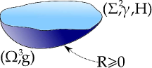
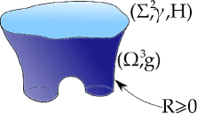
Figure 1. Valid fill-ins of Bartnik data

Interestingly, Bartnik data falls into one of three types. Although trivial to prove, the following fact motivates much of the present paper.

Observation 4 (Trichotomy of Bartnik data).

Bartnik data $(\Sigma,\gamma,H)$ belongs to exactly one of the following three classes:

1. Negative type: $(\Sigma,\gamma,H)$ admits no valid fill-in.

2. Zero type: $(\Sigma,\gamma,H)$ admits a valid fill-in, but every valid fill-in $(\Omega,g)$ has $\partial\Omega=\Sigma$.

3. Positive type: $(\Sigma,\gamma,H)$ admits a valid fill-in $(\Omega,g)$ with nonempty minimal boundary $\partial\Omega\setminus\Sigma$.

Outline.

In section 2, we give some geometric characterizations of valid fill-ins of Bartnik data of zero and positive type, making connections with static vacuum metrics. We also recall in section 2.3 the Bartnik inner mass, which explains the use of the words positive, zero, and negative in the trichotomy.

The essential idea of this paper, presented in section 3, is to study the behavior of Bartnik data $(\Sigma,\gamma,\lambda H)$, where the real parameter $\lambda>0$ is allowed to vary. We show in Theorem 11, the main result, that the data passes through all three classes of the trichotomy, with interesting behavior at some unique borderline value $\lambda=\lambda_{0}$. In section 3.1, we introduce a function that probes the geometry of valid fill-ins of $(\Sigma,\gamma,\lambda H)$.

The main application occurs in section 4, where we use the number $\lambda_{0}$ to define a quasi-local mass for regions in 3-manifolds of nonnegative scalar curvature (Definition 14). Several properties are shown to hold, including nonnegativity. What distinguishes this definition from most others is its tendency to vanish on static vacuum, as opposed to flat, data. We give a brief physical argument for why such a property may be desirable in section 4.1.

Section 5 consists of examples of Bartnik data of all three types, and compares our definition with the Hawking mass and Brown–York mass. In section 6 we introduce a general construction for “twisting” two quasi-local mass functionals together, of which the above quasi-local mass is a special case. The final section is a discussion of some potentially interesting open problems.

Acknowledgements.

The author is indebted to Hubert Bray for suggesting the main idea of varying the parameter $\lambda$. He would like to thank the referee for carefully reading the work and offering a number of thoughtful suggestions.

2. Fill-ins of nonnegative type and the inner mass

2.1. Zero type data and static vacuum metrics

First, we classify the geometry of valid fill-ins of Bartnik data of zero type. Recall that a Riemannian 3-manifold $(\Omega,g)$ is static vacuum if there exists a function $u\geq 0$ (called the static potential), with $u>0$ on the interior of $\Omega$, such that the Lorentzian metric

$$h=-u^{2}dt^{2}+g$$

on $\mathbb{R}\times\operatorname{int}(\Omega)$ has zero Ricci curvature. This condition is equivalent to the system of equations:

$$\Delta u =0$$ (1)

$$u\operatorname{Ric} =\operatorname{Hess}u$$ (2)

where $\Delta,\operatorname{Ric}$ and $\operatorname{Hess}$ are the Laplacian, Ricci curvature, and Hessian with respect to $g$. Equation (1) together with the trace of (2) shows that static vacuum metrics have zero scalar curvature. The following result is primarily a consequence of Corvino’s work on local scalar curvature deformation [corvino].

Proposition 5.

If ${\mathcal{B}}$ is Bartnik data of zero type, then any valid fill-in is static vacuum.

The idea of the proof is to use a valid fill-in that is not static vacuum to construct a valid fill-in that contains a black hole. By a very rough analogy, one might think of this physically as taking some of the energy content in a fill-in and squeezing it down into a black hole. The delicate issue is that we must preserve the boundary data in the process.

Proof.

Let $(\Omega,g)$ be a valid fill-in of zero type data $(\Sigma,\gamma,H)$. By definition, $\partial\Omega=\Sigma.$

We claim $g$ has identically zero scalar curvature. If not, there exists $p\in\operatorname{int}(\Omega)$ and $r>0$ such that on the closed metric ball $\overline{B}(p,r)$, the scalar curvature of $g$ is bounded below by some $\epsilon>0$. On the set $\overline{B}(p,r/2)\setminus\{p\}$, let $G$ be a Green’s function for the Laplacian that blows up at $p$ and vanishes on $\partial\overline{B}(p,r/2)$ (see Theorem 4.17 of [aubin].) By the maximum principle, $G$ is positive, except on $\partial\overline{B}(p,r/2)$. Extend $G$ by zero to the rest of $\Omega\setminus\{p\}$, so that $G$ Lipschitz, smooth away from $\partial\overline{B}(p,r/2)$. Perturb $G$ to a smooth, nonnegative function $\tilde{G}$ on $\Omega\setminus\{p\}$ that agrees with $G$ except possibly on the annular region $\overline{B}(p,3r/4)\setminus\overline{B}(p,r/4)$. For a parameter $\delta>0$ to be determined, define the conformal metric

$$\tilde{g}=(1+\delta\tilde{G})^{4}g$$

on $\Omega\setminus\{p\}$. By construction, $\tilde{g}=g$ outside $\overline{B}(p,r)$ and thus has nonnegative scalar curvature outside this ball. For points inside $\overline{B}(p,r)$, we apply the rule for the change in scalar curvature under a conformal deformation (see appendix A):

$$\tilde{R} =(1+\delta\tilde{G})^{-5}(-8\Delta(1+\delta\tilde{G})+(1+\delta\tilde{G})R)$$

$$\geq(1+\delta\tilde{G})^{-5}(-8\delta\Delta\tilde{G}+\epsilon),$$

Here, $\tilde{R}$ and $R$ are the scalar curvatures of $\tilde{g}$ and $g$. Since $\Delta\tilde{G}$ has compact support, we may choose $\delta>0$ sufficiently small so that the above is strictly positive. In particular, $\tilde{R}\geq 0$ on $\Omega\setminus\{p\}$.

Now, suppose $s$ is the distance function with respect to $g$ from the point $p$. For $s$ sufficiently small, $G$ is of the form $\frac{c}{s}+O(1)$ for some constant $c>0$. The normal derivative of $G$ to the sphere of radius $s$ about $p$ in the outward direction is $-\frac{c}{s^{2}}+O(s^{-1})$ (see Proposition 4.12 and Theorem 4.13 of [aubin]). The mean curvature of the sphere of radius $s$ with respect to $g$ is $\frac{2}{s}+O(1)$ (by Lemma 3.4 of [fan_shi_tam]), and so the mean curvature of this sphere with respect to $\tilde{g}$ is (using appendix A):

$$(1+\delta\tilde{G})^{-3}\left((2s^{-1}+O(1))(1+\delta cs^{-1}+O(1))-4\delta cs^{-2}+O(s^{-1})\right).$$

The dominant term is $-2\delta cs^{-2}$, so that for some $s>0$ sufficiently small, $\partial\overline{B}(p,s)$ has negative mean curvature (with respect to $\tilde{g}$) in direction pointing away from $p$. Let $\tilde{\Omega}$ be $\Omega\setminus B(p,s)$, and restrict $\tilde{g}$ to $\tilde{\Omega}$.

The manifold $(\tilde{\Omega},\tilde{g})$ has boundary with two connected components, both of positive mean curvature in the outward direction. By Lemma 6 below, $(\tilde{\Omega},\tilde{g})$ contains a subset that is a valid fill-in of $(\Sigma,\gamma,H)$ with a minimal boundary component. This contradicts the assumption that the Bartnik data is of zero type, and so we have proved the claim that $g$ is scalar-flat.

Finally, if $(\Omega,g)$ is not static vacuum, then Corvino proves the existence of a metric $\overline{g}$ on $\Omega$ with nonnegative, scalar curvature, positive at some interior point $p$, such that $g-\overline{g}$ is supported away from $\partial\Omega$ [corvino]. In particular, $(\Omega,\overline{g})$ is a valid fill-in for the type-zero data $(\Sigma,\gamma,H)$, and the above argument leads to a contradiction. ∎

To complete the proof of the previous proposition, we have the following lemma:

Lemma 6.

Suppose ${\mathcal{B}}=(\Sigma,\gamma,H)$ admits a fill-in $(\Omega,g)$ with nonnegative scalar curvature, such that $\partial\Omega\setminus\Sigma$ has positive mean curvature in the outward direction. Then a subset $\Omega^{\prime}$ of $\Omega$ is a valid fill-in of ${\mathcal{B}}$ with metric $g|_{\Omega^{\prime}}$. Moreover, $\Omega^{\prime}$ has at least one minimal boundary component.

Proof.

By assumption $\Sigma$ has positive mean curvature $H$ and $\partial\Omega\setminus\Sigma$ has positive mean curvature. By Theorem 19 in appendix B, there exists a smooth, embedded minimal surface $S$ homologous to $\Sigma$. The closure of the region bounded between $\Sigma$ and $S$ is the desired valid fill-in. ∎

2.2. Data of positive type

Proposition 7.

Given Bartnik data ${\mathcal{B}}$, the following are equivalent:

1. ${\mathcal{B}}$ is of positive type.

2. ${\mathcal{B}}$ admits a valid fill-in that has positive scalar curvature at some point.

3. ${\mathcal{B}}$ admits a valid fill-in that has positive scalar curvature everywhere.

The idea of proving the proposition is to create positive energy density at some interior points at the expense of decreasing the size of the minimal surface. As in the previous section, the delicate issue is preserving the boundary data in the process.

Proof.

If ${\mathcal{B}}$ admits a valid fill-in with positive scalar curvature at a point, then ${\mathcal{B}}$ is of nonnegative type and Proposition 5 rules out the case of zero type (since static vacuum metrics have zero scalar curvature). This shows $(2)$ implies $(1)$; $(3)$ trivially implies $(2)$.

Last, we show $(1)$ implies $(3)$. Suppose ${\mathcal{B}}=(\Sigma,\gamma,H)$ has positive type, so there exists some valid fill-in $(\Omega,g)$ of ${\mathcal{B}}$ with boundary $\Sigma\dot{\cup}S$, where $S$ is a nonempty minimal surface. If $(\Omega,g)$ is not static vacuum, we may complete the proof by again using the work of Corvino to perturb $(\Omega,g)$ to a valid fill-in with positive scalar curvature at a point [corvino]. Thus, assume $(\Omega,g)$ is static vacuum, and so in particular it is scalar-flat.

Replace $(\Omega,g)$ with its double across the minimal surface $S$. Now, $(\Omega,g)$ has two boundary components $\Sigma$ and $\Sigma^{\prime}$ (its reflected copy), and contains a minimal surface $S$ that is fixed by the $\mathbb{Z}_{2}$ reflection symmetry. Moreover, $g$ is Lipschitz continuous across $S$ and smooth elsewhere. For simplicity of exposition, we separately treat the cases in which $g$ is smooth and non-smooth across $S$.

Smooth case: For $\epsilon\in(0,1)$, let $\varphi$ be the function on $\Omega$ solving the following Dirichlet problem:

$$\begin{cases}\Delta\varphi=0&\text{ on }\Omega,\\ \varphi=1&\text{ on }\Sigma,\\ \varphi=1-\epsilon&\text{ on }\Sigma^{\prime}.\end{cases}$$

Consider the conformal metric $\tilde{g}=\varphi^{4}g$, which is smooth with zero scalar curvature. Moreover, the mean curvature $\tilde{H}$ of $\Sigma$ with respect to $\tilde{g}$ strictly exceeds $H$ (for all choices of $\epsilon$), since $\varphi$ has positive outward normal derivative on $\Sigma$ (see appendix A). The mean curvature of $\Sigma^{\prime}$ remains positive for $\epsilon>0$ sufficiently small. Fix such an $\epsilon$. This construction is demonstrated in figure LABEL:fig_reflection.

Figure 2. Construction in proof of Proposition 7

Fix any smooth function $\rho>0$ on $\Omega$. For all $\delta\geq 0$ small, let $u_{\delta}$ be the unique solution to the elliptic problem

$$\begin{cases}\tilde{L}u_{\delta}=\delta\rho&\text{ in }\tilde{\Omega},\\ u_{\delta}=1&\text{ on }\Sigma,\\ \partial_{\nu}(u_{\delta})=0&\text{ on }\Sigma^{\prime},\end{cases}$$

where $\tilde{L}=-8\tilde{\Delta}$ is the conformal Laplacian of $\tilde{g}$. Clearly $u_{0}\equiv 1$, and $u_{\delta}$ converges in $C^{2}$ to 1 as $\delta\to 0^{+}$. For $\delta>0$ small enough to ensure $u_{\delta}>0$, the conformal metric $u_{\delta}^{4}\tilde{g}$ has:

• positive scalar curvature (equal to $\delta\rho u_{\delta}^{-5}$),

• induced metric on $\Sigma$ equal to $\gamma$ (by the boundary condition $u_{\delta}|_{\Sigma}=1$),

• positive mean curvature on $\Sigma^{\prime}$ (by the boundary condition $\partial_{\nu}(u_{\delta})|_{\Sigma^{\prime}}=0$), and

• mean curvature on $\Sigma$ converging uniformly to $\tilde{H}$ as $\delta\to 0^{+}$.

Fix a particular value of $\delta$ such that the mean curvature of $\Sigma^{\prime}$ is positive and the mean curvature $\tilde{H}_{\delta}$ of $\Sigma$ is pointwise greater than $H$ (which is possible, since $\tilde{H}>H$). By Lemma 6, there is a valid fill-in of $(\Sigma,\gamma,\tilde{H}_{\delta})$ that contains a minimal surface. By Lemma 20 in appendix C, this valid fill-in can be perturbed to a valid fill-in of $(\Sigma,\gamma,H)$ so that the latter fill-in still has positive scalar curvature.

Lipschitz case: In general we must carry out an extra step to deal with the lack of smoothness across $S$. Define $\varphi$ analogously by first solving $\Delta\varphi_{1}=0$ with boundary conditions of $1$ on $\Sigma$ and $1-\frac{\epsilon}{2}$ on $S$, then defining $\varphi_{2}=2-\epsilon-\varphi_{1}$ in the reflected copy. The function $\varphi$ obtained by gluing $\varphi_{1}$ and $\varphi_{2}$ is $C^{1,1}$ on $\Omega$, and smooth and harmonic away from $S$. Again, let $\tilde{g}=\varphi^{4}g$, which has zero scalar curvature (away from $S$), is Lipschitz across $S$, and induces the same mean curvature on both sides of $S$. Fix $\epsilon>0$ so that $\tilde{H}>H$ and the $\tilde{g}$-mean curvature of $\Sigma^{\prime}$ is positive.

By the work of Miao [miao], the fact that both sides of $S$ have the same mean curvature implies the existence of a family of $C^{2}$ metrics $\{\tilde{g}_{\delta}\}_{0<\delta<\delta_{0}}$ such that

1. $\tilde{g}_{\delta}$ converges to $\tilde{g}$ in $C^{0}$ as $\delta\to 0^{+}$,

2. $\tilde{g}_{\delta}$ agrees with $\tilde{g}$ outside a $\delta$-neighborhood of $S$, and

3. the scalar curvature $\tilde{R}_{\delta}$ of $\tilde{g}_{\delta}$ is bounded below by a constant independent of $\delta$.

In particular, the $L^{p}$ norm of $\tilde{R}_{\delta}$ (taken with respect to $\tilde{g}$ or $\tilde{g}_{\delta}$) for any $1\leq p<\infty$ converges to zero as $\delta\to 0$. We mimic arguments of Schoen and Yau [schoen_yau] to prove:

Lemma 8.

For each $\delta>0$ sufficiently small, the conformal Laplacian $\tilde{L}_{\delta}=-8\tilde{\Delta}_{\delta}+\tilde{R}_{\delta}$ of $\tilde{g}_{\delta}$ has trivial kernel on the space of functions $v$ with boundary conditions of $v=0$ on $\Sigma$ and $\partial_{\nu}v=0$ on $\Sigma^{\prime}$.

Proof.

Let $v$ belong to the kernel of $\tilde{L}_{\delta}$ with the above boundary conditions. Multiplying $\tilde{L}_{\delta}v$ by $v$ and integrating by parts gives

$$0=\int_{\Omega}\left(8|\nabla v|^{2}_{\tilde{g}_{\delta}}+\tilde{R}_{\delta}v^{2}\right)d\tilde{V}_{\delta}.$$

Let $\tilde{R}_{\delta}^{-}=-\min(\tilde{R}_{\delta},0)$, so that

$$\int_{\Omega}8|\nabla v|^{2}_{\tilde{g}_{\delta}}d\tilde{V}_{\delta} \leq\int_{\Omega}\tilde{R}_{\delta}^{-}v^{2}d\tilde{V}_{\delta}$$

$$\leq\left(\int_{\Omega}(\tilde{R}_{\delta}^{-})^{3/2}d\tilde{V}_{\delta}\right)^{2/3}\left(\int_{\Omega}v^{6}d\tilde{V}_{\delta}\right)^{1/3}$$

$$\leq c\left(\int_{\Omega}(\tilde{R}_{\delta}^{-})^{3/2}d\tilde{V}_{\delta}\right)^{2/3}\left(\int_{\Omega}|\nabla v|_{\tilde{g}_{\delta}}^{2}d\tilde{V}_{\delta}\right),$$

having used the Hölder and Sobolev inequalities (where $c>0$ is a constant). Thus, for $\delta$ sufficiently small, a nonzero $v$ may not exist, since the $L^{3/2}$ norm of $\tilde{R}_{\delta}^{-}$ converges to zero. ∎

Fix a smooth function $\rho>0$ on $\Omega$. By the lemma and standard elliptic theory, for $\delta>0$ small there exists unique solution $u_{\delta}$ to the problem:

$$\begin{cases}\tilde{L}_{\delta}u_{\delta}=\delta\rho&\text{ in }\tilde{\Omega},\\ u_{\delta}=1&\text{ on }\Sigma,\\ \partial_{\nu}(u_{\delta})=0&\text{ on }\Sigma^{\prime}.\end{cases}$$

A key fact is that $u_{\delta}$ converges to 1 in $C^{0}$ as $\delta\to 0^{+}$, and this convergence is $C^{2}$ away from $S$ (see the proof of Proposition 4.1 of Miao [miao]).

At this point, the proof follows nearly the same steps as in the smooth case, where we work with the metric $u_{\delta}^{4}\tilde{g}_{\delta}$ (which has positive scalar curvature and induces the metric $\gamma$ on $\Sigma$). We pick $\delta>0$ sufficiently small so that $\tilde{H}_{\delta}>H$ and $\Sigma^{\prime}$ has positive mean curvature with respect to $u_{\delta}^{4}\tilde{g}_{\delta}$. Now, if necessary, perturb the $C^{2}$ metric $u_{\delta}^{4}\tilde{g}_{\delta}$ on a neighborhood of $S$ to a $C^{\infty}$ metric, preserving the above properties. The proof now goes as in the smooth case, making use of Lemmas 6 and 20. ∎

We remark that our assumption of positive Gauss curvature of $(\Sigma,\gamma)$ is not necessary in Propositions 5 and 7.

2.3. Bartnik inner mass

One source of inspiration for the problem of considering valid fill-ins with minimal boundary is Bray’s definition of the Bartnik inner mass [bray_RPI], an example of a quasi-local mass (see section 4 for more on quasi local mass). The Bartnik inner mass aims to measure the size of the largest black hole that could be placed inside a valid fill-in of given Bartnik data.

Definition 9.

The Bartnik inner mass of Bartnik data ${\mathcal{B}}$ is the real number

$$m_{inner}({\mathcal{B}})=\sup_{(\Omega,g)}\left\{\sqrt{\frac{A}{16\pi}}\right\}$$

where the supremum is taken over the class of all valid fill-ins $(\Omega,g)$ of ${\mathcal{B}}$, and $A$ is the minimum area in the homology class of $\Sigma$ in $(\Omega,g)$.

This definition, though formulated differently, is equivalent to Bray’s. The purpose of using the minimum area in the homology class of $\Sigma$ is to ignore any large minimal surfaces “hidden behind” a smaller minimal surface.

We observe that the sign of $m_{inner}({\mathcal{B}})$ corresponds directly to the type of the Bartnik data ${\mathcal{B}}$. To see this, first note that for fill-ins with a minimal boundary, the minimum area of $A$ in the homology class of $\Sigma$ in $(\Omega,g)$ is always attained by a smooth minimal surface, and so $A$ is positive (see Theorem 19). For fill-ins without boundary, $\Sigma$ is homologically trivial, and so $A=0$. Thus, $m_{inner}({\mathcal{B}})$ is positive if ${\mathcal{B}}$ is of positive type; zero if ${\mathcal{B}}$ is of zero type; and $-\infty$ if ${\mathcal{B}}$ is of negative type.

3. The interval of positivity

The following idea was suggested by Bray: as a function of a parameter $\lambda>0$, consider the Bartnik data $(\Sigma,\gamma,\lambda H)$. The main purpose of this section is to state and prove Theorem 11, which partially answers the question of how the type of the data depends on $\lambda$.

One key ingredient is the following well-known theorem of Shi and Tam.

Theorem 10 (Shi–Tam, 2002 [shi_tam]).

If Bartnik data $(\Sigma,\gamma,H)$ has a valid fill-in $(\Omega,g)$, then

$$\int_{\Sigma}(H_{0}-H)dA_{\gamma}\geq 0,$$ (3)

where $H_{0}$ is the mean curvature of an isometric embedding of $(\Sigma,\gamma)$ into Euclidean space $\mathbb{R}^{3}$, and $dA_{\gamma}$ is the area form on $\Sigma$ with respect to the metric $\gamma$. Moreover, equality holds if and only if $(\Omega,g)$ is isometric to a subdomain of $\mathbb{R}^{3}$.

Recall that we assume $\gamma$ to have positive Gauss curvature, which is necessary for the theorem: $H_{0}$ is well-defined, since an isometric embedding of a positive Gauss curvature surface into $\mathbb{R}^{3}$ exists and is unique up to rigid motions (see the references in [shi_tam]).

In our case, inequality (3), which depends only on the Bartnik data, must be satisfied for data that admits a valid fill-in. In particular, by increasing $H$ (while keeping $\gamma$, and therefore $H_{0}$, fixed), it is clear that some Bartnik data do not possess fill-ins (i.e., are of negative type). Hence, the Shi–Tam theorem gives an obstruction to Bartnik data being of nonnegative type.

The following main theorem demonstrates that there exists a unique interval of values of $\lambda$ for which this data $(\Sigma,\gamma,\lambda H)$ is of positive type.

Theorem 11.

Fix Bartnik data $(\Sigma,\gamma,H)$. There exists a unique number $\lambda_{0}>0$ such that $(\Sigma,\gamma,\lambda H)$ is of positive type if and only if $\lambda\in(0,\lambda_{0})$. Moreover, $(\Sigma,\gamma,\lambda H)$ is of negative type if $\lambda>\lambda_{0}$.

As a consequence, $(\Sigma,\gamma,\lambda H)$ is zero type for at most one value of $\lambda$, namely $\lambda_{0}$.

Proof.

Define

$$I_{+} =\{\lambda\in\mathbb{R}^{+}:(\Sigma,\gamma,\lambda H)\text{ is of positive type}\},$$

$$I_{0} =\{\lambda\in\mathbb{R}^{+}:(\Sigma,\gamma,\lambda H)\text{ is of zero type}\},$$

$$I_{\geq 0} =I_{+}\cup I_{0}.$$

Step 1: We first show $I_{+}$ is nonempty. Consider the space $\Omega=\Sigma\times[-1,0]$ with product metric $g$, and identify $\Sigma$ with $\Sigma\times\{0\}$. Let $S$ be the other boundary component of $\Omega$, namely $\Sigma\times\{-1\}$. Observe that 1) $\Omega$ has positive scalar curvature since $\Sigma$ has positive Gauss curvature, and 2) all leaves $\Sigma\times\{t\}$ are minimal surfaces.

Choose a smooth function $v$ on $\Omega$ satisfying the following properties: $v\leq 0$, $v$ vanishes on $\Sigma$ and in a neighborhood of $S$, and $\partial_{\nu}v=\frac{1}{4}H$ on $\Sigma$. For $\epsilon>0$, let $u_{\epsilon}=1+\epsilon v$. In particular, $u_{\epsilon}$ is positive for $\epsilon>0$ sufficiently small. Consider the conformal metric $g_{\epsilon}=u_{\epsilon}^{4}g$. Note that $g_{\epsilon}$ induces the metric $\gamma$ on $\Sigma$, and assigns the following value to the mean curvature of $\Sigma$:

$$H_{\epsilon}=4\partial_{\nu}(u_{\epsilon})=4\epsilon\partial_{\nu}v=\epsilon H,$$

by our choice of $v$. Moreover, the scalar curvature of $g_{\epsilon}$ is

$$R_{g_{\epsilon}} =u_{\epsilon}^{-5}\left(-8\Delta_{g}u_{\epsilon}+R_{g}u_{\epsilon}\right)$$

$$=u_{\epsilon}^{-5}\left(-8\epsilon\Delta_{g}v+R_{g}u_{\epsilon}\right),$$

which is positive for $\epsilon$ sufficiently small, since $R_{g}>0$ and $u_{\epsilon}$ is uniformly bounded below as $\epsilon\to 0^{+}$. Fix such an $\epsilon$. We can see $(\Omega,g_{\epsilon})$ is a valid fill-in of $(\Sigma,\gamma,\epsilon H)$, since this fill-in has positive scalar curvature, induces the correct boundary geometry on $\Sigma$, and $S$ is minimal (since $g_{\epsilon}=g$ near $S$). In particular, $\epsilon$ belongs to $I_{+}$, so $I_{+}\neq\varnothing$.

Step 2: The next step is to show that $I_{\geq 0}$ is connected, and $I_{0}$ contains at most one point. To accomplish this, we show that for every number in $I_{\geq 0}$, every smaller positive number belongs to $I_{+}$. It suffices to show that if $(\Sigma,\gamma,H)$ is of nonnegative type, then $(\Sigma,\gamma,\lambda H)$ is of positive type for all $\lambda\in(0,1)$. This fact follows from the next lemma, by Proposition 7.

Lemma 12.

Let $(\Omega,g)$ be a fill-in of arbitrary Bartnik data $(\Sigma,\gamma,H)$. Fix $\lambda\in(0,1)$ and a neighborhood $U$ of $\Sigma$ in $\Omega$. There exists a metric $\tilde{g}$ on $\Omega$ such that:

1. $\tilde{g}$ is a fill-in of $(\Sigma,\gamma,\lambda H)$,

2. $\tilde{g}\geq g$, with equality outside $U$, and

3. $R_{\tilde{g}}\geq\min(0,R_{g})$ pointwise, with strict inequality on a neighborhood of $\Sigma$, where $R$ and $R_{\tilde{g}}$ are the scalar curvature of $g$ and $\tilde{g}$.

In particular, if $(\Omega,g)$ is a valid fill-in, so is $(\Omega,\tilde{g})$.

Proof.

Working in a neighborhood of $\Sigma$ in $\Omega$ diffeomorphic to $(-t_{0},0]\times\Sigma$ and contained in $U$, we may assume $g$ takes the form

$$g=dt^{2}+G_{t},$$

where $t$ is the negative of $g$-distance to $\Sigma$, and $G_{t}$ is a Riemannian metric on the surface $\Sigma_{t}=\Sigma\times\{t\}$. Shrinking $t_{0}$ if necessary, we may assume that every $(\Sigma_{t},G_{t})$ has positive Gauss curvature $K_{t}$ and positive mean curvature $H_{t}$ (in the outward direction $\partial_{t}$). Let $\rho:(-t_{0},0]\to\mathbb{R}$ be a smooth function satisfying

1. $\rho\equiv 1$ in a neighborhood of $-t_{0}$,

2. $\rho(0)=\lambda^{-1}>1$,

3. $\rho^{\prime}(t)\geq 0$, and

4. $\rho^{\prime}(0)>0$.

Define a new metric $\tilde{g}$ on $\Omega$ by setting

$$\tilde{g}=\rho(t)^{2}dt^{2}+G_{t}$$ (4)

on the neighborhood of $\Sigma$, and extending smoothly by $g$ to the rest of $\Omega$; claim (b) is satisfied. A straightforward calculation shows that $\Sigma$ has mean curvature $\lambda H$ in the metric $\tilde{g}$; moreover $\tilde{g}$ induces the metric $\gamma$ on $\Sigma$, so claim (a) holds. Last, we must study the scalar curvature of $\tilde{g}$ on the neighborhood $(-t_{0},0]\times\Sigma$. The following well-known formula, obtained from computing the variation of mean curvature under a unit normal flow, gives the scalar curvature of $g$ as:

$$R_{g}=-2\frac{\partial H_{t}}{\partial t}+2K_{t}-H_{t}^{2}-\|h_{t}\|^{2},$$ (5)

where $h_{t}$ is the second fundamental form of $\Sigma_{t}$ in $(\Omega,g)$, and its norm $\|\cdot\|^{2}$ is taken with respect to $G_{t}$. Applying this formula to the metric $\tilde{g}$ yields

$$R_{\tilde{g}}=\frac{1}{\rho(t)^{2}}R_{g}+2K_{t}(1-\rho(t)^{-2})+2\frac{\rho^{\prime}(t)}{\rho(t)^{3}}H_{t}.$$ (6)

Now, $K_{t}>0,\rho(t)\geq 1,\rho^{\prime}(t)\geq 0$ and $H_{t}>0$, so we see $R_{\tilde{g}}(x)\geq 0$ if $R_{g}(x)\geq 0$ and $R_{\tilde{g}}(x)\geq R_{g}(x)$ if $R_{g}(x)<0$; both are strict inequalities near $t=0$, proving claim (c). ∎

We conclude that $I_{\geq 0}$ is a convex subset of $\mathbb{R}^{+}$, containing all arbitrarily small positive numbers. Moreover, $I_{0}$ contains at most a single point.

Step 3: We prove that $I_{\geq 0}$ is bounded above. This follows immediately from the work of Shi and Tam. More precisely, if $\lambda\in I_{\geq 0}$, then

$$\lambda\leq\frac{\int_{\Sigma}H_{0}dA_{\gamma}}{\int_{\Sigma}HdA_{\gamma}}.$$

Together with step 2, we see $I_{\geq 0}$ and $I_{+}$ are intervals of the form $(0,\lambda_{0}]$ or $(0,\lambda_{0})$.

Step 4: Here we prove that $\lambda_{0}$ does not belong to $I_{+}$. If $\lambda_{0}\in I_{+}$, then by Proposition 7, there exists a valid fill-in $(\Omega,g)$ of $(\Sigma,\gamma,\lambda_{0}H)$ with positive scalar curvature at some point and boundary $\Sigma\dot{\cup}S_{0}$, with $S_{0}$ minimal and nonempty. Solve the mixed Dirichlet–Neumann problem:

$$\begin{cases}\Delta u=\frac{1}{8}R_{g}u&\text{ in }\Omega,\\ u=1&\text{ on }\Sigma,\\ \partial_{\nu}(u)=0&\text{ on }S_{0}.\end{cases}$$ (7)

Here, $\nu$ is the unit normal, always chosen to point out of $\Omega$. Note that a solution exists because $R_{g}\geq 0$. By the maximum principle, $u>0$ in $\Omega$ and $\partial_{\nu}(u)>0$ on $\Sigma$. Let $g^{\prime}=u^{4}g$. Note that $g^{\prime}$ has zero scalar curvature, induces the metric $\gamma$ on $\Sigma$ and assigns zero mean curvature to $S_{0}$. In particular, if we let $H^{\prime}$ be the mean curvature of $\Sigma$ with respect to $g^{\prime}$, then $(\Sigma,\gamma,H^{\prime})$ has a valid fill-in with minimal boundary, namely $(\Omega,g^{\prime})$, and is therefore of positive type. Observe that $H^{\prime}>\lambda_{0}H$. Choose $\beta>1$ so that $H^{\prime}>\beta\lambda_{0}H$. By Lemma 20 in appendix C, we see that $(\Sigma,\gamma,\beta\lambda_{0}H)$ is of positive type. Therefore $\beta\lambda_{0}\in I_{+}$, which contradicts $\lambda_{0}=\sup I_{+}$. We conclude $I_{+}=(0,\lambda_{0})$, and either $I_{\geq 0}=(0,\lambda_{0})$ or $(0,\lambda_{0}]$. It follows that if $\lambda>\lambda_{0}$, then $(\Sigma,\gamma,\lambda H)$ must be of negative type. ∎

To emphasize the picture, the data $(\Sigma,\gamma,\lambda H)$ is of positive type for $\lambda$ small. As we increase $\lambda$, this behavior persists until $\lambda=\lambda_{0}$. At this point, the data is zero or negative, and for $\lambda>\lambda_{0}$, the data is negative. See section 7 for further discussion of the behavior near $\lambda=\lambda_{0}$.

3.1. Inner mass function

In the remainder of this section we will study the function

$$m(\lambda)=m_{inner}(\Sigma,\gamma,\lambda H)$$ (8)

defined for $\lambda\in(0,\lambda_{0})$. Intuitively, one would expect the following behavior of the function $m(\lambda)$. For $\lambda$ small, the mean curvature $\lambda H$ is close to zero, so one might anticipate the existence of a valid fill-in with minimal boundary of approximately the same area as $\Sigma$.

As $\lambda$ increases, one would expect the class of valid fill-ins to shrink; one reason is that the Shi–Tam inequality is more difficult to satisfy. Consequently, the Bartnik inner mass ought to decrease as well. The following statement supports this intuition.

Proposition 13.

Given Bartnik data $(\Sigma,\gamma,H)$, the function $m:(0,\lambda_{0})\to\mathbb{R}^{+}$ is continuous and decreasing, with the following limiting behavior:

$$\lim_{\lambda\to 0^{+}}m(\lambda)=\sqrt{\frac{|\Sigma|_{\gamma}}{16\pi}}.$$

Here, $|\Sigma|_{\gamma}$ is the area of $\Sigma$ with respect to $\gamma$.

Proof.

Monotonicity: Given $0<\lambda_{1}<\lambda_{2}<\lambda_{0}$, we showed in Lemma 12 that any valid fill-in of $(\Sigma,\gamma,\lambda_{2}H)$ gives rise to a valid fill-in of $(\Sigma,\gamma,\lambda_{1}H)$ with a metric that is pointwise at least as large (see (4)). From the definition of the Bartnik inner mass, this shows that

$$m(\lambda_{1})\geq m(\lambda_{2}).$$

Continuity: Suppose $0<\lambda_{1}<\lambda_{0}$, and let $\epsilon>0$. From the definition of the Bartnik inner mass, there exists a valid fill-in $(\Omega,g)$ of $(\Sigma,\gamma,\lambda_{1}H)$ whose minimum area $A$ in the homology class of $\Sigma$ satisfies

$$m(\lambda_{1})-\sqrt{\frac{A}{16\pi}}<\frac{\epsilon}{3}.$$

From Proposition 7, there exists a valid fill-in $(\tilde{\Omega},\tilde{g})$ of $(\Sigma,\gamma,\lambda_{1}H)$ that has strictly positive scalar curvature, and whose minimum area $\tilde{A}$ in the homology class of $\Sigma$ is close to $A$:

$$\sqrt{\frac{A}{16\pi}}-\sqrt{\frac{\tilde{A}}{16\pi}}<\frac{\epsilon}{3}.$$

Now, for $\lambda_{0}>\lambda>\lambda_{1}$, $(\tilde{\Omega},\tilde{g})$ can be perturbed to a fill-in $(\tilde{\Omega},\tilde{g}_{\lambda})$ of $(\Sigma,\gamma,\lambda H)$ using a metric of the form $(\ref{eqn_warped_metric})$. The scalar curvature of $\tilde{g}_{\lambda}$ has potentially decreased relative to that of $\tilde{g}$, but remains positive for $\lambda>\lambda_{1}$ sufficiently close to $\lambda_{1}$. Since $\tilde{g}_{\lambda}\to\tilde{g}$ in $C^{0}$, we may assume $\lambda-\lambda_{1}$ is small enough so that

$$\sqrt{\frac{\tilde{A}}{16\pi}}-\sqrt{\frac{\tilde{A}_{\lambda}}{16\pi}}<\frac{\epsilon}{3},$$

where $\tilde{A}_{\lambda}$ is the minimum $\tilde{g}_{\lambda}$-area in the homology class of $\Sigma$. Adding the last three inequalities and using the definition of the Bartnik inner mass gives

$$m(\lambda_{1}) <\epsilon+\sqrt{\frac{\tilde{A}_{\lambda}}{16\pi}}$$

$$\leq\epsilon+m(\lambda)$$

for $\lambda-\lambda_{1}$ sufficiently small. Together with the fact that $m(\cdot)$ is decreasing, we have shown $m(\cdot)$ is continuous at $\lambda_{1}$.

Lower limit behavior: To study the behavior of $m(\epsilon)$ for $\epsilon$ small, recall that in Step 1 of the proof of Theorem 11 we constructed a valid fill-in of $(\Sigma,\gamma,\epsilon H)$ by a metric $g_{\epsilon}$ uniformly close (controlled by $\epsilon$) to a cylindrical product metric $g$ over $(\Sigma,\gamma)$. As $\epsilon\to 0^{+}$, the minimum $g_{\epsilon}$ area in the homology class of $\Sigma$ converges to the minimum $g$-area in the same homology class, which is $|\Sigma|_{\gamma}$. On the other hand, the Bartnik inner mass of $(\Sigma,\gamma,H^{\prime})$ (for any $H^{\prime}$) never exceeds $\sqrt{\frac{|\Sigma|_{\gamma}}{16\pi}}$ by definition. This proves

$$\lim_{\lambda\to 0+}m(\lambda)=\sqrt{\frac{|\Sigma|_{\gamma}}{16\pi}}.$$

∎

In section 7 we conjecture that $m(\lambda)$ limits to zero as $\lambda\to\lambda_{0}^{-}$, behavior supported by the explicit computation of $m(\lambda)$ in a spherically-symmetric case in section 5.1.

4. Quasi-local mass

Recall from the introduction the problem of assigning a “quasi-local mass” to a bounded region $\Omega$ in a totally geodesic spacelike slice $(M,g)$ of a spacetime. By most definitions, the quasi-local mass of $\Omega$ depends only on the Bartnik data $(\Sigma,\gamma,H)$ of the boundary, and we adopt this perspective here. That is, we define a quasi-local mass functional to be a map from (a subspace of) the set of Bartnik data to the real numbers. We refer the reader to [sza] for a recent comprehensive survey of quasi-local mass.

We begin by recalling some well-known examples of quasi-local mass. First, the Hawking mass of $(\Sigma,\gamma,H)$ is defined to be

$$m_{H}(\Sigma,\gamma,H)=\sqrt{\frac{|\Sigma|_{\gamma}}{16\pi}}\left(1-\frac{1}{16\pi}\int_{\Sigma}H^{2}dA_{\gamma}\right).$$

There is no correlation between the sign of the Bartnik data and the sign of the Hawking mass. That is, the Hawking mass can be negative for positive Bartnik data, and vice versa (see section 5).

Next, the Brown–York mass is defined for Bartnik data $(\Sigma,\gamma,H)$ (assuming as we do that $K_{\gamma}>0$ and $H>0$) by

$$m_{BY}(\Sigma,\gamma,H)=\frac{1}{8\pi}\int_{\Sigma}(H_{0}-H)dA_{\gamma},$$

where $H_{0}$ is the mean curvature of an isometric embedding of $(\Sigma,\gamma)$ into $\mathbb{R}^{3}$. Theorem 10 of Shi–Tam establishes that the Brown–York mass is nonnegative for Bartnik data of nonnegative type. However, there exist Bartnik data of both negative and zero type for which the Brown–York mass is strictly positive (see section 5).

A third example is the Bartnik inner mass, defined in section 2.3.

A key observation is that Theorem 11 canonically associates to any Bartnik data (with $H>0$ and $K_{\gamma}>0$) a positive number $\lambda_{0}$, which we call the critical parameter. In this section we use $\lambda_{0}$ to construct a new example of a quasi-local mass functional.

To motivate this definition, we will compute the number $\lambda_{0}$ for concentric round spheres $\Sigma_{r}$ in the Schwarzschild manifold of mass $m$, with induced metric $\gamma_{r}$ and mean curvature $H_{r}$. For our purposes the Schwarzschild manifold of mass $m$ is $\mathbb{R}^{3}$ minus the open Euclidean ball of radius $m/2$, where $m>0$, equipped with the metric

$$g=\left(1+\frac{m}{2r}\right)^{4}\delta,$$ (9)

where $\delta$ is the Euclidean metric. Note that $g$ is scalar-flat and its boundary is a minimal 2-sphere, called the horizon.

Straightforward computations show that $(\Sigma_{r},\gamma_{r})$ is a round sphere of area $4\pi r^{2}\left(1+\frac{m}{2r}\right)^{4}$, and

$$H_{r}=\frac{2}{r}\left(1+\frac{m}{2r}\right)^{-2}-\frac{2m}{r^{2}}\left(1+\frac{m}{2r}\right)^{-3},$$

having used (19). The mean curvature $H_{r}^{0}$ of $(\Sigma_{r},\gamma_{r})$ embedded in $\mathbb{R}^{3}$ is

$$H_{r}^{0}=\frac{2}{r}\left(1+\frac{m}{2r}\right)^{-2}.$$

Therefore, if we let $\lambda_{r}=H_{r}^{0}/H_{r}$, then $(\Sigma_{r},\gamma_{r},\lambda_{r}H_{r})$ admits a valid fill-in – namely a closed ball in flat-space of boundary area $4\pi r^{2}\left(1+\frac{m}{2r}\right)^{4}$. On the other hand, if $\lambda$ belongs to the interval of positivity for $(\Sigma_{r},\gamma_{r},H_{r})$, then by Shi–Tam

$$\lambda\leq\frac{\int_{\Sigma}H_{r}^{0}dA_{\gamma}}{\int_{\Sigma}H_{r}dA_{\gamma}}=\lambda_{r}.$$

Thus, $\lambda_{r}$ is the critical parameter for the Bartnik data. Some simplifications show

$$\lambda_{r}=\frac{1+\frac{m}{2r}}{1-\frac{m}{2r}}.$$ (10)

In particular, we have the identity in Schwarzschild space:

$$m=\sqrt{\frac{|\Sigma_{r}|_{g}}{16\pi}}\left(1-\frac{1}{\lambda_{r}^{2}}\right),$$

for all values of $r$, motivating the following definition of quasi-local mass.

Definition 14.

Let ${\mathcal{B}}=(\Sigma,\gamma,H)$ be Bartnik data with critical parameter $\lambda_{0}$ (from Theorem 11). Define

$$m({\mathcal{B}})=m(\Sigma,\gamma,H)=\sqrt{\frac{|\Sigma|_{\gamma}}{16\pi}}\left(1-\frac{1}{\lambda_{0}^{2}}\right).$$

Recall that we assume $\gamma$ has positive Gauss curvature and $H>0$.

Theorem 15.

Definition 14 of quasi-local mass satisfies the following properties:

1. (nonnegativity) If Bartnik data ${\mathcal{B}}$ admits a valid fill-in, then its mass $m({\mathcal{B}})$ is nonnegative and is zero only if every valid fill-in is static vacuum.

2. (spherical symmetry) If Bartnik data ${\mathcal{B}}$ arises from a coordinate sphere in a Schwarzschild metric of mass $m$, then $m({\mathcal{B}})=m$.

3. (black hole limit). If ${\mathcal{B}}_{n}=(\Sigma,\gamma,H_{n})$ is a sequence of Bartnik data and $H_{n}\to 0$ uniformly, then

   $$\lim_{n\to\infty}m({\mathcal{B}}_{n})=\sqrt{\frac{|\Sigma|_{\gamma}}{16\pi}}.$$

4. (ADM-sub-limit) If $(M,g)$ is an asymptotically flat manifold with nonnegative scalar curvature, and if $S_{r}$ is a coordinate sphere of radius $r$ with induced metric $\gamma_{r}$ and mean curvature $H_{r}$, then

   $$m_{ADM}(M,g)\geq\limsup_{r\to\infty}m(S_{r},\gamma_{r},H_{r}).$$ (11)

Remarks.

The proof of Theorem 15 uses the positive mass theorem [schoen_yau] implicitly, via Lemma 16 below, which relies on the theorem of Shi–Tam. On the other hand Theorem 15 also recovers the positive mass theorem: if $(M,g)$ is asymptotically flat, has nonnegative scalar curvature, with $\partial M$ empty or consisting of minimal surfaces, then by property (1), $m(S_{r})\geq 0$ for all $S_{r}$. From this, inequality (11) gives $m_{ADM}\geq 0$.

Proof.

Nonnegativity: Observe the following four statements are equivalent, using Theorem 11: $m({\mathcal{B}})>0$; $\lambda_{0}>1$; the number $1$ belongs to the interval of positivity $I_{+}$; ${\mathcal{B}}$ is of positive type. Also, if $(\Sigma,\gamma,H)$ is of zero type, then $\lambda_{0}=1$ (as follows from Theorem 11), so $m({\mathcal{B}})$ vanishes. On the other hand, if $m({\mathcal{B}})$ vanishes, then $\lambda_{0}=1$, so the data is either negative or zero (again, by Theorem 11). But if it is given that the data admits a fill-in, then the data must be of zero type. By Proposition 5, any such fill-in is static vacuum.

Spherical symmetry: This is clear from the construction at the beginning of this section; we defined quasi-local mass so that it has this property.

Black hole limit: It is straightforward to check that if $H_{n}\to 0$ uniformly, then the sequence of critical parameters $\lambda_{n}$ diverges to infinity.

ADM-sub-limit: For all $r$ sufficiently large, the coordinate spheres $S_{r}$ have positive mean and Gauss curvatures. To prove (11), recall that the Brown–York mass limits to the ADM mass in the sense that

$$m_{ADM}(M,g)=\lim_{r\to\infty}m_{BY}(S_{r}).$$

(See Theorem 1.1 of [fan_shi_tam] and the references therein.) Since we assume $(M,g)$ has nonnegative scalar curvature, $S_{r}$ is of positive or zero type for all $r$ for which the coordinate sphere is defined. We invoke Lemma 16 below, which states $m(S_{r})\leq m_{BY}(S_{r})$, completing the proof. ∎

Lemma 16.

For Bartnik data ${\mathcal{B}}=(\Sigma,\gamma,H)$ of nonnegative type,

$$m({\mathcal{B}})\leq m_{BY}({\mathcal{B}}).$$

Proof.

Let $H_{0}$ be the mean curvature of an isometric embedding of $(\Sigma,\gamma)$ in $\mathbb{R}^{3}$, which is well-defined because $K_{\gamma}>0$. By Shi–Tam, we have $\lambda_{0}\leq\frac{\int_{\Sigma}H_{0}dA_{\gamma}}{\int_{\Sigma}HdA_{\gamma}}$. In particular,

$$m({\mathcal{B}}) =\sqrt{\frac{|\Sigma|_{\gamma}}{16\pi}}\left(1-\frac{1}{\lambda_{0}^{2}}\right)$$

$$\leq\sqrt{\frac{|\Sigma|_{\gamma}}{16\pi}}\left(1-\left(\frac{\int_{\Sigma}HdA_{\gamma}}{\int_{\Sigma}H_{0}dA_{\gamma}}\right)^{2}\right)$$ (12)

$$\leq\sqrt{\frac{|\Sigma|_{\gamma}}{16\pi}}\left(\frac{\left(\int_{\Sigma}H_{0}dA_{\gamma}+\int_{\Sigma}HdA_{\gamma}\right)\left(\int_{\Sigma}H_{0}dA_{\gamma}-\int_{\Sigma}HdA_{\gamma}\right)}{\left(\int_{\Sigma}H_{0}dA_{\gamma}\right)^{2}}\right)$$

$$\leq\sqrt{\frac{|\Sigma|_{\gamma}}{16\pi}}\frac{16\pi m_{BY}({\mathcal{B}})}{\int_{\Sigma}H_{0}dA_{\gamma}},$$

where again we have used Shi–Tam and the fact that the data is of nonnegative type. The Minkowski inequality for convex regions in $\mathbb{R}^{3}$ [isoperimetric] states that

$$\left(\int_{\Sigma}H_{0}dA_{\gamma}\right)^{2}\geq 16\pi|\Sigma|_{\gamma}.$$

Together with the above, this completes the proof. ∎

The right-hand side of (12) is a definition of quasi-local mass proposed by Miao, which he observed is bounded above by the Brown–York mass using the same argument [miao_local_rpi].

4.1. Physical remarks

It has been suggested in the literature (see [bartnik_3_metrics] for instance) that if the quasi-local mass of the boundary of a region $\Omega$ vanishes, then $\Omega$ ought to be flat. The Brown–York mass and Bartnik mass both satisfy this property (see [bartnik_mass, imcf]). Definition 14 suggests an alternative viewpoint that such $\Omega$ ought to be static vacuum, which includes flat metrics as a special case. Indeed, one could make a physical argument that in a region of a spacetime that is static vacuum, quasi-local mass should vanish since there is no matter content and no gravitational dynamics (cf. [anderson], which also discusses the vanishing of quasi-local mass on static vacuum regions).

5. Examples

Let $(M,g)$ be a Riemannian 3-manifold. If $\Omega$ is a subset of $M$ with boundary $\partial\Omega$ homeomorphic to $S^{2}$, and if $\partial\Omega$ has positive mean curvature $H$ (with respect to some chosen normal direction), define

$$m(\Omega)=m(\partial\Omega,g_{T\partial\Omega},H),$$

where $T\partial\Omega$ is the tangent bundle of $\partial\Omega$. If $g$ has nonnegative scalar curvature, then $m(\Omega)\geq 0$ by Theorem 15.

Euclidean space: Consider $\mathbb{R}^{3}$ with the standard flat metric. Let $\Omega\subset\mathbb{R}^{3}$ be a strictly convex open set with smooth boundary that is not round, with mean curvature $H_{0}$ and induced metric $\gamma_{0}$. There is no valid fill-in of $(\partial\Omega,\gamma_{0},H_{0})$ with mean curvature $H>H_{0}$; this statement follows from the Shi–Tam inequality (3) or alternatively by Miao’s “positive mass theorem with corners” [miao]. This implies $\lambda_{0}=1$, and so $m(\Omega)=0$. The Brown–York mass of $\Omega$ also vanishes, as $H_{0}=H$. A straightforward computation shows that the Hawking mass of $\Omega$ is strictly negative.

Schwarzschild, positive mass: Next let $(M,g)$ be a Schwarzschild manifold of mass $m>0$ (see equation (9)). Suppose $\Omega\subset M$ is topologically an open 3-ball with boundary $\Sigma$ disjoint from the horizon.

Lemma 17.

For the Bartnik data induced on $\partial\Omega$, $\lambda_{0}=1$. Equivalently, $m(\Omega)=0$.

Figure LABEL:fig_schwarz gives a depiction of the Bartnik data in question.

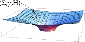
Figure 3. Off-center ball in Schwarzschild

Proof.

Certainly $\lambda_{0}\geq 1$, since $\Omega$ is tautologically a valid fill-in. If $\lambda_{0}>1$, there exists a valid fill-in $\Omega^{\prime}$ of $\Sigma$ (with the same boundary metric and mean curvature), such that $\partial\Omega^{\prime}\setminus\Sigma$ is nonempty and consists of minimal surfaces. Glue $\Omega^{\prime}$ to $M\setminus\Omega$ along $\Sigma$, obtaining a manifold $(M^{\prime},g^{\prime})$ that is smooth and has nonnegative scalar curvature away from $\Sigma$. Moreover, $g^{\prime}$ is Lipschitz across $S$, and $\partial M^{\prime}$ consists of minimal surfaces (including the Schwarzschild horizon). Let $A$ and $A^{\prime}$ be the minimum areas in the homology class of the boundary for the respective manifolds $(M,g)$ and $(M^{\prime},g^{\prime})$. $A$ is attained uniquely by the horizon $S$ in $M$, and by a similar consideration $A^{\prime}$ is attained by a surface $S^{\prime}$ that includes $S$ as a proper subset. (To see this, observe that the Schwarzschild manifold minus its horizon is foliated by the $\{r=\text{const.}\}$ spheres, which are convex; thus $S^{\prime}$ may not intersect the interior of $M^{\prime}\setminus\Omega$ yet must intersect $M^{\prime}\setminus\Omega$ to be homologous to the boundary of $M^{\prime}$.) Thus $A^{\prime}>A$. By direct computation,

$$m=\sqrt{\frac{A}{16\pi}},$$

and so

$$m^{\prime}<\sqrt{\frac{A^{\prime}}{16\pi}},$$ (13)

where $m^{\prime}=m$ is the ADM mass of $(M^{\prime},g^{\prime})$ (equal because $g$ and $g^{\prime}$ agree outside a compact set). Using an argument similar to Miao [miao], one can mollify $(M^{\prime},g^{\prime})$ to a smooth, asymptotically flat metric of nonnegative scalar curvature and minimal boundary that gives strict inequality in (13). This violates the well-known Riemannian Penrose inequality [imcf, bray_RPI]. This contradiction implies that $\lambda_{0}=1$, so $m(\Omega)=0$. ∎

Thus, we have examples of Bartnik data of zero type that do not arise as the boundaries of regions in flat space. In other words, we have non-flat domains $\Omega$ for which $m(\Omega)=0$. Of course, by Theorem 15, such $\Omega$ must be static vacuum (as is the case for the Schwarzschild metric).

To further extend this example, Huisken and Ilmanen [imcf] show that there exist small balls $\Omega$ away from the horizon in the Schwarzschild manifold whose Bartnik data $(\Sigma,\gamma,H)$ have strictly positive Hawking mass. Moreover, the case of equality of Theorem 10 of Shi and Tam shows that the Brown–York mass of $\Omega$ is also strictly positive. It follows that for $\lambda>1$ sufficiently close to 1, the data $(\Sigma,\gamma,\lambda H)$ is of negative type, yet still has strictly positive $m_{H}$ and $m_{BY}$.

Note that we have not stated $\Omega$ being static vacuum implies $m(\Omega)=0$. Counterexamples are unknown to the author.

Schwarzschild, negative mass: Let $(M,g)$ be the Schwarzschild metric of mass $m<0$ (defined by (9) on $\mathbb{R}^{3}$ minus the closed ball of radius $|m|/2$). The Bartnik data induced on spheres $\{r=\text{const.}\}$ is of negative type because the critical parameter $\lambda_{r}$ is less than one by (10).

5.1. Example $m(\lambda)$ function

Here we give an explicit computation of the inner mass function $m(\lambda)$ defined in section 3.1 for Bartnik data ${\mathcal{B}}$ corresponding to the coordinate sphere $S_{r}$ of radius $r>m/2$ in the Schwarzschild metric of mass $m>0$, with induced metric $\gamma$ and mean curvature $H$. The Riemannian Penrose inequality [bray_RPI], shows that the Bartnik inner mass of ${\mathcal{B}}$ equals $m$. Let $\lambda>0$; the data $(S_{r},\gamma,\lambda H)$ embeds uniquely as a coordinate sphere $S_{r^{\prime}}$ of some radius $r^{\prime}$ in a Schwarzschild metric of some mass $m^{\prime}$. Equating the areas of $S_{r}$ and $S_{r^{\prime}}$ in their respective metrics, we have

$$4\pi r^{2}\left(1+\frac{m}{2r}\right)^{4}=4\pi(r^{\prime})^{2}\left(1+\frac{m^{\prime}}{2r^{\prime}}\right)^{4}.$$ (14)

Equating $\lambda H$ with the mean curvature of $S_{r^{\prime}}$ leads to

$$\lambda\left(\frac{2}{r}\left(1+\frac{m}{2r}\right)^{-2}-\frac{2m}{r^{2}}\left(1+\frac{m}{2r}\right)^{-3}\right)=\frac{2}{r^{\prime}}\left(1+\frac{m^{\prime}}{2r^{\prime}}\right)^{-2}-\frac{2m^{\prime}}{(r^{\prime})^{2}}\left(1+\frac{m^{\prime}}{2r^{\prime}}\right)^{-3}.$$ (15)

With some calculations, one can compute $r^{\prime}$ and $m^{\prime}$ explicitly. For $\lambda\in(0,\lambda_{0})$, we know $m(\lambda)$, the Bartnik inner mass of $S_{r^{\prime}}$, simply equals $m^{\prime}$ (again, by the Riemannian Penrose inequality). Omitting some details, we give the formula:

$$m(\lambda)=\frac{r}{2}\left(\left(1+\frac{m}{2r}\right)^{2}-\lambda^{2}\left(1-\frac{m}{2r}\right)^{2}\right).$$ (16)

As anticipated by Proposition 13, $m(\lambda)$ is continuous, decreasing, and $m(0)=\sqrt{\frac{A}{16\pi}}$, where $A$ is the area of $S_{r}$ in the Schwarzschild metric of mass $m$. Moreover, $m(\lambda)$ vanishes at the critical value $\lambda_{0}=\frac{1+\frac{m}{2r}}{1-\frac{m}{2r}}$ (computed in section 4), a property conjectured to hold in general (see the paragraph following Problem 2 in section 7).

6. An algebraic operation on quasi-local mass functionals

For a quasi-local mass functional $m_{i}$ (i.e., a map from the set of Bartnik data to the real numbers), define the following quantity in $[-\infty,\infty]$:

$$\lambda_{i}(\Sigma,\gamma,H)=\sup\{\lambda>0:m_{i}(\Sigma,\gamma,\lambda H)\geq 0\}.$$

In other words, $\lambda_{i}$ measures how much one can scale the boundary mean curvature until the mass $m_{i}$ becomes negative. Up to this point, we have studied this quantity for the case in which $m_{i}$ is the Bartnik inner mass (since $m_{inner}(\Sigma,\gamma,H)\geq 0$ if and only if $(\Sigma,\gamma,H)$ has a valid fill-in). Theorem 11 implies that $\lambda_{i}$ is a positive, finite number for the case $m_{i}=m_{inner}$.

Here we use the number $\lambda_{i}$ to construct an algebraic product of two quasi-local mass functionals, of which that constructed in section 4 is a special case. We restrict to quasi-local mass functionals $m_{i}$ satisfying the following mild assumptions on all Bartnik data:

1. $\lambda_{i}(\Sigma,\gamma,H)$ is a positive real number, and

2. $m_{i}(\Sigma,\gamma,\lambda H)$ is decreasing as a function of $\lambda$.

For example the Hawking mass, Brown–York mass, and Bartnik inner mass (see Proposition 13) satisfy these properties.

Define the following binary operation on the set of quasi-local mass functionals. Given $m_{1}$ and $m_{2}$, let

$$(m_{1}*m_{2})(\Sigma,\gamma,H)=m_{1}\left(\Sigma,\gamma,\frac{\lambda_{1}}{\lambda_{2}}H\right),$$ (17)

where $\lambda_{i}=\lambda_{i}(\Sigma,\gamma,H)$ for $i=1,2$. This operation satisfies a number of properties.

Proposition 18.

Let $m_{1},m_{2},$ and $m_{3}$ be quasi-local mass functionals.

1. $m_{1}*m_{1}=m_{1}$.

2. $(m_{1}*m_{2})*m_{3}=m_{1}*m_{3}=m_{1}*(m_{2}*m_{3})$. In particular, $*$ is associative.

3. $m_{2}$ controls the sign of $m_{1}*m_{2}$ in the following sense:

   1. $m_{1}*m_{2}(\Sigma,\gamma,H)>0$ if and only if $m_{2}(\Sigma,\gamma,H)>0$, and

   2. $m_{1}*m_{2}(\Sigma,\gamma,H)=0$ if and only if $m_{2}(\Sigma,\gamma,H)=0$.

4. If $m_{1}$ has the black hole limit property (see Theorem 15), so does $m_{1}*m_{2}$.

5. If both $m_{1}$ and $m_{2}$ produce the value $m$ on concentric round spheres in the Schwarzschild metric of mass $m$, then so does $m_{1}*m_{2}$.

6. If $m_{2}\leq m_{3}$ (as functions), then $m_{1}*m_{2}\leq m_{1}*m_{3}$.

The above properties all essentially follow immediately from the definitions and so we omit the proof. Below we sketch some of the steps as a sample.

Sketch:.

We compute $(m_{1}*m_{2})*m_{3}$. First, $(m_{1}*m_{2})(\Sigma,\gamma,H)=m_{1}(\Sigma,\gamma,\frac{\lambda_{1}}{\lambda_{2}}H)$ has critical parameter $\lambda_{2}$. Then

$$((m_{1}*m_{2})*m_{3}(\Sigma,\gamma,H)) =(m_{1}*m_{2})\left(\Sigma,\gamma,\frac{\lambda_{2}}{\lambda_{3}}H\right)$$

$$=m_{1}\left(\Sigma,\gamma,\frac{\lambda_{1}}{\lambda_{2}}\frac{\lambda_{2}}{\lambda_{3}}H\right),$$

which equals $(m_{1}*m_{3})(\Sigma,\gamma,H)$.

We also demonstrate property (3a). Note $(m_{1}*m_{2})(\Sigma,\gamma,H)=m_{1}(\Sigma,\gamma,\frac{\lambda_{1}}{\lambda_{2}}H)$ is positive if and only if $\frac{\lambda_{1}}{\lambda_{2}}<\lambda_{1}$; that is, $\lambda_{2}>1$. However, $\lambda_{2}>1$ if and only if $m_{2}(\Sigma,\gamma,H)>0$. ∎

In the next section, we demonstrate $m_{1}*m_{2}$ generally does not equal $m_{2}*m_{1}$.

6.1. Examples of $m_{1}*m_{2}$

 

Hawking mass and Bartnik inner mass: The quasi-local mass of Definition 14 is equal to $m_{H}*m_{inner}$, where $m_{H}$ is the Hawking mass. To see this, note that $\lambda_{H}=\sqrt{\frac{16\pi}{\int_{\Sigma}H^{2}dA_{\gamma}}}$ and $\lambda_{inner}=\lambda_{0}$. Then by definition,

$$m_{H}*m_{inner}(\Sigma,\gamma,H) =m_{H}\left(\Sigma,\gamma,\frac{\lambda_{H}}{\lambda_{0}}H\right)$$

$$=\sqrt{\frac{|\Sigma|_{\gamma}}{16\pi}}\left(1-\frac{1}{\lambda_{0}^{2}}\right).$$

We reiterate that $m_{H}*m_{inner}$ inherits the following property from $m_{inner}$: vanishing precisely on Bartnik data of zero type.

Hawking mass and Brown–York mass: To compute $m_{H}*m_{BY}$, we note $\lambda_{H}$ was found in the last example, and $\lambda_{BY}=\frac{\int_{\Sigma}H_{0}dA_{\gamma}}{\int_{\Sigma}HdA_{\gamma}}.$ Using the definition,

$$m_{H}*m_{BY}(\Sigma,\gamma,H)=\sqrt{\frac{|\Sigma|_{\gamma}}{16\pi}}\left(1-\left(\frac{\int_{\Sigma}HdA_{\gamma}}{\int_{\Sigma}H_{0}dA_{\gamma}}\right)^{2}\right).$$

This quasi-local mass was written down in a different context by Miao [miao_local_rpi].

Brown–York mass and Hawking mass: The steps from the last example show

$$m_{BY}*m_{H}(\Sigma,\gamma,H)=\int_{\Sigma}H_{0}dA_{\gamma}\left(1-\sqrt{\frac{\int_{\Sigma}H^{2}dA_{\gamma}}{16\pi}}\right),$$

illustrating concretely the non-commutativity of $*$.

7. Concluding remarks and open problems

We conclude by mentioning some questions raised in this paper.

Problem 1.

Determine whether the quasi-local mass of Definition 14 is monotone under some flow.

Monotonicity means that if $\{(\Sigma_{t},\gamma_{t},H_{t})\}_{t\in[0,\epsilon)}$ is some family of surfaces (together with their Bartnik data) moving outward in a manifold of nonnegative scalar curvature, then $m(\Sigma_{t},\gamma_{t},H_{t})$ is non-decreasing. Monotonicity is often (but not universally) suggested as a desirable property of quasi-local mass [bartnik_3_metrics].

Problem 2.

Determine whether the Bartnik data $(\Sigma,\gamma,\lambda_{0}H)$ is of zero type. Equivalently, construct a static vacuum fill-in of $(\Sigma,\gamma,\lambda_{0}H)$.

That the two above statements are equivalent follows from Proposition 5 and Theorem 11. The precise nature of the Bartnik data rescaled with the critical parameter $\lambda_{0}$ is perhaps the biggest open question of this paper. An affirmative answer to Problem 2 would imply that $(\Sigma,\gamma,\lambda_{0}H)$ admits a static vacuum fill-in. In general, constructing static vacuum metrics with prescribed boundary data is a very difficult problem (cf. the work of Anderson and Khuri on static vacuum asymptotically flat “extensions” of Bartnik data [ak]).

More generally, one could ask what happens to the geometry of the class valid fill-ins of $(\Sigma,\gamma,\lambda H)$ in the limit $\lambda\nearrow\lambda_{0}$. An optimistic conjecture would be that in the limit $\lambda\nearrow\lambda_{0}$, any valid fill-in $(\Omega_{\lambda},g_{\lambda})$ of $(\Sigma,\gamma,\lambda H)$ satisfies:

• the black holes (area-minimizing minimal surfaces) in $(\Omega_{\lambda},g_{\lambda})$ are shrinking to zero size (i.e., $\lim_{\lambda\to\lambda_{0}^{-}}m(\lambda)=0$), and

• the metric $g_{\lambda}$ is approaching a static vacuum metric in an appropriate sense.

There may be a connection between the first point and Miao’s localized Riemannian Penrose inequality [miao_local_rpi].

The above discussion is basically a localization of the near-equality case of the positive mass theorem [schoen_yau]. In such a global setting, the question is: what happens to the geometry of a sequence of asymptotically flat manifolds $(M_{i},g_{i})$ of nonnegative scalar curvature whose total mass is approaching zero? The Riemannian Penrose inequality [imcf, bray_RPI] shows that any black holes in $(M_{i},g_{i})$ must be approaching zero, and some partial results exist for proving that $g_{i}$ is approaching a flat metric [bartnik_tsing, dan_lee, bray_finster, lee_sormani].

Appendix A Conformal transformation of curvatures

We repeatedly used the following formulas that relate the scalar curvature and mean curvature of conformal metrics. Suppose $g$ and $\overline{g}$ are Riemannian metrics on a 3-manifold for which $\overline{g}=u^{4}g$ for some smooth function $u>0$. If $R$ and $\overline{R}$ are the scalar curvatures of $g$ and $\overline{g}$, then

$$\overline{R}=u^{-5}(-8\Delta u+Ru),$$ (18)

where $\Delta$ is the Laplacian with respect to $g$. Next, suppose $S$ is a hypersurface with unit normal field $\nu$ with respect to $g$. Then the mean curvatures $H$ and $\overline{H}$ (in the direction defined by $\nu$) with respect to $g$ and $\overline{g}$ satisfy:

$$\overline{H}=u^{-2}H+4u^{-3}\nu(u).$$ (19)

Appendix B Geometric measure theory

Here is an extremely useful result from geometric measure theory on the existence and regularity of area-minimizing surfaces.

Theorem 19.

Let $(M,g)$ be a smooth, compact Riemannian manifold of dimension $2\leq n\leq 7$ with boundary $\partial M$. Suppose $\partial M$ has positive mean curvature (i.e., inward-pointing mean curvature vector). Given a connected component $S$ of $\partial M$, there exists a smooth, embedded hypersurface $\tilde{S}$ of zero mean curvature that minimizes area among surfaces homologous to $S$. Moreover, $\tilde{S}$ does not intersect $\partial M$.

These results are essentially due to Federer and Fleming [fed_flem, fleming, federer]. The rough idea of the proof of Theorem 19 is to take a minimizing sequence of surfaces $\{S_{i}\}$ (viewed as integral currents) in $[S]$, the homology class of $S$. By the Federer–Fleming compactness theorem, some subsequence converges to a surface $\tilde{S}$. Standard arguments show that $\tilde{S}$ remains in $[S]$ and indeed has the desired minimum of area. Regularity theory (requiring $n\leq 7$) proves that $\tilde{S}$ is a smooth, embedded hypersurface. By the first variation of area formula, $\tilde{S}$ has zero mean curvature and may not touch the positive mean curvature boundary (which acts as a barrier). See the appendix of [schoen_yau] for a careful proof of the last fact.

Appendix C Deformations of scalar curvature near a boundary

Here we prove the following useful lemma.

Lemma 20.

Suppose that $(\Sigma,\gamma,H_{1})$ admits a valid fill-in. If $0<H_{2}<H_{1}$, then $(\Sigma,\gamma,H_{2})$ admits a valid fill-in with positive scalar curvature at a point. In particular, $(\Sigma,\gamma,H_{2})$ is of positive type.

Although we only prove the case $K_{\gamma}>0$ here, Lemma 20 is true without this hypothesis. The proof is an application of techniques developed recently by Brendle, Marques, and Neves [bmn].

Proof.

Step 1: We construct a valid fill-in of $(\Sigma,\gamma)$ with mean curvature strictly greater than $H_{2}$ and with positive scalar curvature in a neighborhood of $\Sigma$.

Since $\Sigma$ is compact, we may choose $\alpha\in(0,1)$ so that $\alpha H_{1}>H_{2}$. We proved in step 2 of Theorem 11 that $(\Sigma,\gamma,\alpha H_{1})$ is of positive type and moreover admits a valid fill-in $(\Omega,g_{1})$ whose scalar curvature is strictly positive in a neighborhood $U$ of $\Sigma$. (For the latter statement, refer to equation (6) and note that $\rho^{\prime}(0)>0$.)

Step 2: We define a metric $g_{2}$ on $\Omega$ as follows, with the goal of making the boundary mean curvature of $g_{2}$ equal to $H_{2}$. First, consider a neighborhood of $\Sigma$ contained in $U$ that is diffeomorphic to $\Sigma\times(-t_{0},0]$ (where $t=0$ corresponds to $\Sigma$). Define for $x\in\Sigma$ and $t\in(-t_{0},0]$:

$$g_{2}(x,t)=\rho(t)^{2}dt^{2}+(1+tH_{2}(x))\gamma(x),$$

where $\rho(t)$ is a function satisfying $\rho(0)=1$ and will be specified later. It is readily checked that $g_{2}$ induces on $\Sigma$ the metric $\gamma$ and mean curvature $H_{2}$. Shrinking $t_{0}$ if necessary and choosing $\rho(t)$ bounded below by a positive constant with $\rho^{\prime}(t)>0$ sufficiently large, we may arrange $g_{2}$ to have strictly positive scalar curvature on $\Sigma\times(-t_{0},0]$. This is readily checked using equation (5). Now, extend $g_{2}$ arbitrarily to a smooth metric on $\Omega$ (not necessarily preserving nonnegative scalar curvature). Replace $U$ with the smaller neighborhood $\Sigma\times(-t_{0},0]$

To summarize, we have two metrics $g_{1}$ and $g_{2}$ on the compact manifold $\Omega$, inducing boundary data $(\Sigma,\gamma,\alpha H_{1})$ and $(\Sigma,\gamma,H_{2})$, respectively, each with positive scalar curvature on the neighborhood $U$ of $\Sigma$. By compactness, the scalar curvatures of $g_{1}|_{U}$ and $g_{2}|_{U}$ are bounded below by a constant $R_{0}>0$.

Step 3: Apply Theorem 5 of Brendle–Marques–Neves [bmn] to produce a metric $\hat{g}$ on $\Omega$ satisfying the following properties:

1. $R_{\hat{g}}(x)\geq\min\{R_{g_{1}}(x),R_{g_{2}}(x)\}-\frac{R_{0}}{2}$,

2. $\hat{g}$ agrees with $g_{1}$ outside of $U$,

3. $\hat{g}$ agrees with $g_{2}$ in some neighborhood of $\Sigma$.

(To apply the theorem, it is crucial that $\alpha H_{1}>H_{2}$.)

By the third condition, $(\Omega,\hat{g})$ is a fill-in of $(\Sigma,\gamma,H_{2})$. By the first and second conditions, $\hat{g}$ has nonnegative (but not identically zero) scalar curvature and $\partial\Omega\setminus\Sigma$ (if nonempty) is a minimal surface. In particular, $(\Omega,\hat{g})$ is a valid fill-in with positive scalar curvature at some point.

Finally, the last statement in the lemma follows from Proposition 7. ∎