Neutrino masses and mixings in the baryon triality constrained minimal supersymmetric standard model

Abstract

We discuss how the experimental neutrino oscillation data can be realized in the framework of the baryon triality ($B_{3}$) constrained supersymmetric Standard Model (cSSM). We show how to obtain phenomenologically viable solutions, which are compatible with the recent WMAP observations. We present results for the hierarchical, inverted and degenerate cases which illustrate the possible size and structure of the lepton number violating couplings. We work with a new, as yet unpublished version of SOFTSUSY  where we implemented full one–loop neutrino masses. Finally, we shortly discuss some phenomenological implications at the LHC.

I Introduction

Experimentally, it is well established that the Standard Model (SM) of particle physics requires an extension to accommodate the neutrino oscillation data Davis:1968cp ; Fukuda:1998ah ; Fukuda:1998fd ; Ahmad:2002jz ; Aharmim:2005gt ; Apollonio:2002gd ; Cleveland:1998nv . The data indicate that at least two neutrinos are massive and that the neutrino mixing angles are large. Many mechanisms have been proposed to explain the neutrino mass pattern. The simplest is to introduce small Dirac mass terms. However, in order to be compatible with observations, the Yukawa couplings can at most be of $\mathcal{O}(10^{-12})$, which appears highly unnatural. Furthermore, this requires additional right–handed neutrinos and the corresponding Majorana mass terms are unconstrained by SM gauge symmetries.

Alternatively, one can allow for the Majorana mass terms, this is the so–called (type–I) see–saw mechanism Minkowski:1977sc ; Mohapatra:1979ia ; Yanagida ; GellMann:1980vs ; Mohapatra:1980yp ; Jezabek:1998du . By setting the arbitrary Majorana mass scale to be large, light neutrinos with mass of order $\mathcal{O}({\rm 0.1\,eV})$ can be obtained even with $\mathcal{O}(1)$ Yukawa couplings. There are other see–saw mechanisms Magg:1980ut ; Lazarides:1980nt ; Schechter:1980gr ; Mohapatra:1980yp ; Foot:1988aq ; Mohapatra:1986aw ; Mohapatra:1986bd ; Dreiner:1994ra , which involve different additional particles that determine/control the see–saw scale. Some models, involving a see–saw mechanism, determine the detailed neutrino masses from a broken (gauge) symmetry Zee:1980ai ; Dreiner:1992zy ; Ibanez:1994ig ; Dreiner:1994ra ; Dreiner:2003yr ; He:2003rm ; Luhn:2007sy ; Dreiner:2007vp .

In this paper we consider a natural mechanism in supersymmetric extensions of the SM, which does not require any right–handed, gauge singlet, neutrinos, or a corresponding new mass scale. We restrict ourselves to the minimal particle content, consisting of the SM particles, an additional Higgs SU(2)_L doublet, and their superpartners, i.e. the supersymmetric Standard Model (SSM) Nilles:1983ge ; Haber:1984rc ; Drees:1996ca . The most general gauge invariant and renormalizable SSM Lagrangian contains lepton number violating (LNV) operators which mix the left–handed neutrinos with the neutralinos. The neutralino mass provides a see–saw scale, of $\mathcal{O}({\rm 100\,GeV})$, for the generation of light Majorana neutrino masses Hall:1983id ; Joshipura:1994ib ; Nowakowski:1995dx ; Grossman:1997is ; Grossman:1999hc ; Grossman:2000ex ; Nardi:1996iy ; Davidson:2000ne ; Dedes:2006ni ; Dreiner:2007uj ; Allanach:2007qc .

In the generic SSM, there exist LNV and baryon number violating operators. We thus restrict our model to conserve baryon triality ($B_{3}$) Ibanez:1991hv ; Ibanez:1991pr ; Banks:1991xj ; Dreiner:2005rd ; Dreiner:2006xw . This prohibits all baryon number violating terms while allowing for lepton number violation, and the proton is stable. Furthermore, we work in the constrained baryon triality SSM ($B_{3}$ cSSM) in order to limit the number of free (lepton number conserving) parameters at the unification scale. The relevant details of this model are presented in the next section. It is well–known that in the $B_{3}$ cSSM, only one light neutrino is massive at tree–level Hall:1983id ; Joshipura:1994ib ; Nowakowski:1995dx ; Nardi:1996iy ; Davidson:2000ne ; Dedes:2006ni ; Abada:1999ai ; Dreiner:2007uj . Higher order corrections need to be included to give mass to at least one more neutrino in order to be consistent with the non–zero values of the neutrino mass squared differences, $\Delta m_{21}^{2}$ and $\Delta m_{31}^{2}$. The radiative origin of the second neutrino mass scale implies that a strong hierarchy of $\mathcal{O}(100)$ between the neutrino masses is to be expected, cf. Ref. Allanach:2007qc . However, the data require a neutrino mass ratio of the heaviest two neutrinos of at most $\mathcal{O}(5)$.

Thus a mechanism is needed to suppress the tree–level mass scale for viable models. In Ref. Allanach:2007qc , sets of five parameters [two trilinear LNV couplings together with three mixing angles that describe the charged lepton Yukawa matrix] defined in a cSSM were found to reproduce the oscillation data. The LNV parameters were chosen such that their contributions to the tree–level neutrino masses partially cancel against each other. Another possibility, first mentioned in Ref. deCarlos:1996du , is that the tree–level neutrino mass can vanish in a more generic fashion in certain regions of cSSM parameter space, specified by the trilinear soft supersymmetry breaking parameter $A_{0}$. A detailed explanation of how this situation arises, including a discussion on loop contributions in this parameter space was presented in Ref. Dreiner:2010ye .

In this paper, we focus especially on these parameter regions, and aim to reproduce the neutrino oscillation data using a small set of LNV couplings. Compared with Ref. Allanach:2007qc , these regions might be considered more preferable in the sense that they avoid suppression of tree level neutrino masses through specific cancellations between LNV parameters. Our set–up is also different from Ref. Allanach:2007qc , in that we specify the LNV parameters in a basis where the lepton Yukawa couplings are diagonal. We consider this advantageous, as this allows for a more transparent understanding and better control of how different LNV parameters contribute to the neutrino mass matrix. Here we also improve on the numerical calculation performed in Ref. Allanach:2007qc by including a full one loop calculation for the sneutrino vacuum expectation values, on top of the one loop corrections to the neutral fermion masses. This computation is implemented as an extension to the mass spectrum calculational tool SOFTSUSY Allanach:2001kg ; Allanach:2009bv .

Our aim is to obtain the correct masses and mixing angles with a small number of LNV parameters. We furthermore wish to analyze the general structures that lead to potential solutions, since it is not possible to systematically list all solutions. This work is an extension of Ref. Dreiner:2010ye , where single coupling bounds from the cosmological limit on the neutrino mass, Eq. (11), were determined. By introducing parameters coupled to different generations, we attempt to understand how different trilinear LNV terms interplay with each other to generate the observed mass pattern.

The generation of neutrino masses through non–zero LNV parameters directly at the electroweak scale (therefore without the complications from renormalisation group effects) has been studied in Refs. Abada:1999ai ; Dedes:2006ni . Generation of neutrino masses via bilinear LNV couplings and the corresponding collider signatures have also been studied. We refer interested readers to Refs. Bhattacharyya:1996nj ; Dreiner:1997uz ; Barbier:2004ez ; Hempfling:1995wj ; Kaplan:1999ds ; Mira:2000gg ; Hirsch:2002ys ; Hirsch:2000ef ; Diaz:2003as ; Bartl:2003uq ; Hirsch:2003fe ; Hirsch:2004he ; Hirsch:2005ag ; deCampos:2007bn ; deCampos:2008av and references therein.

The outline of this paper is as follows. In section II, we introduce the $B_{3}$ cSSM model, and highlight the most relevant ingredients, including the choice of benchmark scenarios and (low energy) observables that could constrain the LNV parameters, for our present study. In section III we examine in detail sets of LNV parameters that can reproduce the neutrino oscillation data. Section IV is devoted to the numerical fitting procedure used in our analysis. We discuss our best fit parameter sets and possible collider phenomenology in sections V and VI, before concluding in section VII.

II Neutrino Masses in the Baryon Triality ($B_{3}$) cSSM

II.1 Experimental Neutrino Data

The best fit of the combined global analysis of atmospheric, solar, reactor and accelerator data in terms of three active oscillating neutrinos is given by Schwetz:2011qt ; GonzalezGarcia:2010er ,

$$\sin^{2}[\theta_{12}] = 0.31\pm 0.02,$$ (1)

$$\sin^{2}[\theta_{23}] = 0.51\pm 0.06,$$ (2)

$$\sin^{2}[\theta_{13}] < 0.03,$$ (3)

$$\Delta m_{21}^{2} = 7.59\pm 0.2\times 10^{-5}\textrm{ eV}^{2},$$ (4)

$$\Delta m_{31}^{2} = \left\{\begin{array}[]{r}-2.34\pm 0.1\times 10^{-3}\textrm{ eV}^{2}\\ 2.45\pm 0.1\times 10^{-3}\textrm{ eV}^{2}\end{array}\right.,$$ (7)

where the errors are given at the $1\sigma$ level, and

$$\Delta m_{ij}^{2} \equiv m_{i}^{2}-m_{j}^{2}.$$ (8)

The data indicate large mixing angles $\theta_{12}$ and $\theta_{23}$ and a small or possibly even vanishing angle $\theta_{13}$. This implies that at least two neutrinos have non–zero mass. The (as–yet) undetermined sign of $\Delta m_{31}^{2}$ means that two mass orderings are possible. They are known as the normal ($\Delta m_{31}^{2}>0$) and the inverted ($\Delta m_{31}^{2}<0$) hierarchies.

For illustrative purposes, we often use the tri–bi–maximal mixing (TBM) approximation Harrison:2002er , where

$$\sin^{2}[\theta_{12}]=\frac{1}{3},\;\;\sin^{2}[\theta_{23}]=\frac{1}{2}\,\;\;\sin^{2}[\theta_{13}]=0$$ (9)

is assumed. Note that these are all within 1$\,\sigma$ of the best–fit experimental values given in Eqs. (1)–(3). The first two quantities differ from their best fit values by 7% and 2% respectively. In the TBM approximation, the Pontecorvo–Maki–Nakagawa–Sakata (PMNS) mixing matrix Pontecorvo:1957cp ; Maki:1962mu ; Pontecorvo:1967fh is explicitly given by

$$U_{TBM}\equiv\left(\begin{array}[]{ccc}\phantom{-}\sqrt{\frac{2}{3}}&\phantom{-}\sqrt{\frac{1}{3}}&\;\;\;\;\;0\\ -\sqrt{\frac{1}{6}}&\phantom{-}\sqrt{\frac{1}{3}}&\phantom{-}\sqrt{\frac{1}{2}}\\ \phantom{-}\sqrt{\frac{1}{6}}&-\sqrt{\frac{1}{3}}&\phantom{-}\sqrt{\frac{1}{2}}\end{array}\right)\,.$$ (10)

Since the defining equations in Eq. (9) involve squares, more than one phase convention exists for the resulting mixing matrix.

The observations and measurements from neutrino oscillations determine the differences of neutrino masses squared, cf. Eqs. (4), (7). Direct laboratory measurements restrict the absolute masses of the neutrinos to be below $\mathcal{O}(10\,{\rm MeV}-1\,{\rm eV})$ GonzalezGarcia:2010er ; GonzalezGarcia:2007ib ; Barate:1997zg ; Assamagan:1995wb ; Bonn:2001tw ; Lobashev:2001uu ; Amsler:2008zzb . Limits dependent on the Majorana nature of neutrinos also exist from non–observation of neutrinoless double beta decay ($0\nu\beta\beta$), which is of $\mathcal{O}(0.5\,{\rm eV})$ Bakalyarov:2003jk ; KlapdorKleingrothaus:2000sn ; Arnaboldi:2008ds ; Aalseth:2002rf . Note, there is a claim of evidence for a neutrino mass of $0.39\,\mathrm{eV}$ in a $0\nu\beta\beta$ experiment KlapdorKleingrothaus:2001ke .

A stringent upper limit can be obtained from cosmological restrictions on the sum of the neutrino masses, with the exact limit dependent on details of the analysis. Typically these analyses include data from the Wilkinson Microwave Anisotropy Probe (WMAP) Spergel:2006hy , Large Scale Structure SDSS ; 2dFGRS and Type Ia supernovae supernovae . For our purpose, we use

$$\sum{m_{\nu_{i}}}\lesssim 0.4\,\text{eV}\,,$$ (11)

at $99.9\%$ confidence level, obtained from Refs. Cirelli:2006kt ; Goobar:2006xz .

In our numerical fitting procedure, we make use of three limiting cases of neutrino mass hierarchies. In the first two cases, we assume that the lightest neutrino is massless and impose normal and inverted hierarchy, respectively. In the third case, we consider almost–degenerate neutrino masses with normal hierarchy mass ordering, saturating the cosmological limit stated in Eq. (11).

For the normal ($m_{1}<m_{2}<m_{3}$) and inverted ($m_{3}<m_{1}<m_{2}$) hierarchies, neutrino masses are respectively given by

• normal hierarchy (NH):

  $$m_{1} \approx 0\textrm{ eV},$$

  $$m_{2} = 8.71\times 10^{-3}\textrm{ eV},$$

  $$m_{3} = 4.95\times 10^{-2}\textrm{ eV},$$

  $$m_{3}/m_{2} \sim 5.7\,.$$ (12)

• inverted hierarchy (IH):

  $$m_{1} = 4.84\times 10^{-2}\textrm{ eV},$$

  $$m_{2} = 4.92\times 10^{-2}\textrm{ eV},$$

  $$m_{3} \approx 0\textrm{ eV},$$

  $$m_{2}/m_{1} \sim 1\,.$$ (13)

In our fits, we use the masses given in Eqs.(12) and (13) as central values for the three neutrino masses for the NH and IH cases, respectively. For the degenerate case ($m_{1}\approx m_{2}\approx m_{3}$), we assume that the sum of the three active neutrino masses equals $0.4\textrm{ eV}$.

II.2 Baryon Triality ($B_{3}$) cSSM

With the field content of the SSM, the most general gauge invariant superpotential at the renormalizable level can be written as Sakai:1981pk ; Weinberg:1981wj ; Weinberg:1979sa

$$\mathcal{W} = \mathcal{W}_{R_{p}}+\mathcal{W}_{{{\not\!{R}}_{p}}},$$ (14)

where $\mathcal{W}_{R_{p}}$($\mathcal{W}_{{{\not\!{R}}_{p}}}$) contain terms that conserve (violate) the discrete symmetries R–parity ($R_{p}$) as well as proton hexality ($P_{6}$). In a notation that follows Ref. Allanach:2003eb and SOFTSUSY  Allanach:2001kg ; Allanach:2009bv closely, they are

$$\mathcal{W}_{R_{p}} = \epsilon_{ab}\,[(Y_{E})_{jk}H_{d}^{a}L_{j}^{b}\bar{E}_{k}+(Y_{D})_{jk}H_{d}^{a}Q_{j}^{b}\bar{D}_{k}$$ (15)

$$\phantom{\epsilon_{ab}}+(Y_{U})_{jk}Q_{j}^{a}H_{u}^{b}\bar{U}_{k}-\mu H_{d}^{a}H_{u}^{b}],$$

$$\mathcal{W}_{{{\not\!{R}}_{p}}} = \epsilon_{ab}\,[\frac{1}{2}\lambda_{ijk}L_{i}^{a}L_{j}^{b}\bar{E}_{k}+\lambda^{\prime}_{ijk}L_{i}^{a}Q_{j}^{b}\bar{D}_{k}$$ (16)

$$\phantom{\epsilon_{ab}}+\lambda^{\prime\prime}_{ijk}\bar{U}_{i}\bar{D}_{j}\bar{D}_{k}-\kappa_{i}L_{i}^{a}H_{u}^{b}],$$

where $i,j,k\,\in\{1,2,3\}$ are generation indices, $a,b\in\{1,2\}$ ($\epsilon_{12}=1$) are indices of the $SU(2)_{L}$ fundamental representation, while the corresponding $SU(3)_{c}$ indices are suppressed. To avoid operators that could result in dangerously fast proton decay Weinberg:1979sa ; Wilczek:1979hc ; Sakai:1981pk ; Smirnov:1996bg , we impose the discrete symmetry baryon triality ($B_{3}$) Ibanez:1991hv ; Ibanez:1991pr ; Banks:1991xj ; Dreiner:2005rd ; Dreiner:2006xw . Under this symmetry, baryon number is conserved while we have lepton number violation (LNV). The superpotential is given by

$$\mathcal{W}_{B_{3}} = \mathcal{W}_{R_{p}}+\mathcal{W}_{\rm LNV},$$ (17)

where the last term on the right is obtained by setting $\lambda^{\prime\prime}=0$ in $\mathcal{W}_{{{\not\!{R}}_{p}}}$. We note that $R_{p}$, $B_{3}$ and $P_{6}$ are the only discrete symmetries which can be written as a remnant of a broken anomaly free gauge symmetry Ibanez:1991hv ; Ibanez:1991pr ; Dreiner:2005rd ; Banks:1991xj . In the rest of this paper, $B_{3}$ is assumed to be conserved.

The LNV soft supersymmetry (SUSY) breaking interaction Lagrangian is given by

$$-\mathcal{L}_{LNV} = \epsilon_{ab}\,[\frac{1}{2}h_{ijk}\tilde{L}^{a}_{i}\tilde{L}^{b}_{j}\tilde{E}_{k}+h^{\prime}_{ijk}\tilde{L}^{a}_{i}\tilde{Q}^{b}_{j}\tilde{D}_{k}$$ (18)

$$-\tilde{D}_{i}\tilde{L}^{a}_{i}h^{b}_{u}]+m^{2}_{L_{i}H_{d}}\tilde{L}^{\dagger}_{ia}h_{d}^{a}+h.c.,$$

where tilde denotes a super–partner of the more familiar Standard Model field. The complete $R_{p}$ soft SUSY breaking Lagrangian can be found in Ref. Allanach:2001kg .

The $B_{3}$ SSM model has more than 200 free parameters Haber:1997if . In order to perform concrete numerical studies, we restrict our discussion to the cSSM framework Drees:1996ca . The cSSM model is specified by the parameter set

$$M_{0},\quad M_{1/2},\quad A_{0},\quad{\rm sgn}(\mu),\quad{\rm tan}\beta,$$ (19)

denoting the universal scalar mass, the universal gaugino mass, the universal trilinear scalar coupling, the sign of the bilinear Higgs mixing parameter $\mu$ and the ratio of Higgs vacuum expectation values (VEVs) $v_{u}/v_{d}$ at the electroweak scale $M_{Z}$. Except for $\tan\beta$, all parameters are defined at the unification scale $M_{X}$.

Additionally, we allow for a subset of $B_{3}$ conserving (but $R_{p}$–violating) parameters

$${\bf\Lambda}\subset\{\lambda_{ijk},\lambda^{\prime}_{ijk}\}$$ (20)

that will be specified in later sections. Note that we allow for trilinear but not bilinear LNV parameters at the unification scale, because we work in a basis where the bilinear LNV couplings $\kappa_{i}$ and $\tilde{D}_{i}$ are both zero at $M_{X}$. This is possible for universal SUSY breaking Allanach:2003eb via a basis transformation of the lepton and Higgs superfields Hall:1983id ; Dreiner:2003hw . However, at lower energy scales $\kappa_{i}$ and $\tilde{D}_{i}$ are generated via the renormalization group equations (RGEs) Nardi:1996iy .

II.3 Neutrino and Charged Lepton Masses

Since lepton number is violated, the lepton doublet superfields $L_{i}$ carry the same quantum numbers as the down–type $H_{d}$ superfield doublet. As a result, the neutralinos and neutrinos mix:

$$\mathcal{L}_{\mathcal{M}_{N}} = -\frac{1}{2}(\nu_{i},-i\widetilde{B},-i\widetilde{W}^{3},\tilde{h}_{d},\tilde{h}_{u})\mathcal{M}_{N}\left(\begin{array}[]{c}\nu_{j}\\ -i\widetilde{\mathcal{B}}\\ -i\widetilde{\mathcal{W}}^{3}\\ \tilde{h}_{d}\\ \tilde{h}_{u}\end{array}\right)\;.$$ (26)

In the above expression, $\mathcal{M}_{N}$ is a $7\times 7$ mass matrix. As we are interested in models with a strong hierarchy between the mass scales of the neutralinos and the neutrinos, it is convenient to write $\mathcal{M}_{N}$ as

$$\mathcal{M}_{N} = \left(\begin{array}[]{cc}m_{\nu}&m\\ m^{T}&\mathcal{M}_{\chi^{0}}\end{array}\right),$$ (30)

where $m_{\nu}$ is the $3\times 3$ mass matrix in the neutrino sector and $\mathcal{M}_{\chi^{0}}$ is the $4\times 4$ mass matrix in the neutralino sector. $m$ denotes the $3\times 4$ mixing matrix which arises through R–parity violation. An effective neutrino mass matrix $\mathcal{M}_{\nu}^{{\rm eff}}$ can then be defined via the see–saw mechanism

$$\mathcal{M}_{\nu}^{{\rm eff}} \equiv m_{\nu}-m\mathcal{M}_{\chi^{0}}^{-1}m^{T}.$$ (31)

At tree–level, in which $m_{\nu}=0$, it is given by Joshipura:1994ib ; Nowakowski:1995dx

$$(\mathcal{M}_{\nu}^{{\rm eff}})^{\textrm{tree}}_{ij} = \frac{\mu(M_{1}g^{2}_{2}+M_{2}g^{2})}{2v_{u}v_{d}(M_{1}g^{2}_{2}+M_{2}g^{2})-2\mu M_{1}M_{2}}\Delta_{i}\Delta_{j}$$

where

$$\Delta_{i} \equiv v_{i}-v_{d}\frac{\kappa_{i}}{\mu},\qquad i=1,2,3\,.$$ (33)

Here $v_{i}$ and $v_{d}$ are vacuum expectation values (VEVs) of the sneutrino and ($H_{d}$) higgs fields. An effective neutrino mixing matrix $U_{\nu}$ can then be defined via the relation

$$U_{\nu}^{T}\mathcal{M}_{\nu}^{{\rm eff}}U_{\nu} = {\rm diag}[m_{\nu i}],\qquad i=1,2,3.$$ (34)

The rank–1 structure of $(\mathcal{M}_{\nu}^{{\rm eff}})^{\rm tree}$ leads to only one non–zero neutrino mass. In order to fit neutrino oscillation data, which implies at least two massive neutrinos, higher order corrections must be included. In fact, these corrections must be sizable as the mass ratio of the two heaviest neutrinos is of order one, cf. Sect. II.1.

In this paper, we therefore include the full one–loop contributions to the neutrino–neutralino sector. Our calculation follows closely that of Refs. Dedes:2006ni ; Allanach:2007qc . However we go beyond their approximations by including also the 1–loop LNV corrections to the VEVs $v_{i}$, $v_{d}$ and $v_{u}$. This is discussed in more detail in section IV.1.

Beyond tree–level, the matrix $m_{\nu}$ is filled by the loop contributions to the neutrino masses. A good measure of this loop scale is set by contributions from so–called $\Lambda\Lambda$ loops (see Sec. II.5):

$$\phantom{.}(m_{\nu}^{\mathbf{\Lambda\Lambda}})_{ij} = \sum_{k,n}\left(\lambda_{ikn}\lambda_{jnk}A^{l}_{kn}+n_{c}\lambda^{\prime}_{ikn}\lambda^{\prime}_{jnk}A^{d}_{kn}\right),$$ (35)

where $n_{c}=3$ is the color factor, and

$$\phantom{.}A^{f}_{kn} = \frac{1}{32\pi^{2}}m_{f_{k}}\sin 2\tilde{\phi}_{n}^{f}\,\ln\left(\frac{m^{2}_{\tilde{f}_{1n}}}{m^{2}_{\tilde{f}_{2n}}}\right)$$ (36)

$$\sim \frac{1}{16\pi^{2}}m_{f_{k}}m_{f_{n}}\frac{(A_{0}-\mu{\rm tan}\beta)}{m^{2}_{\tilde{f}_{Ln}}-m^{2}_{\tilde{f}_{Rn}}}\ln\left(\frac{m^{2}_{\tilde{f}_{Ln}}}{m^{2}_{\tilde{f}_{Rn}}}\right)$$ (37)

are loop functions for the $k$th generation fermion and $n$th generation sfermions. Here $f=\ell,d$ denotes a charged lepton or a down–like quark. $A^{f}_{kn}$ depends on the fermion mass $m_{f_{k}}$, the mixing angle $\tilde{\phi}^{f}_{n}$ for the rotation of the left– and right– handed sfermion current eigenstates to the two mass eigenstates, and the sfermion masses $m_{\tilde{f}_{1n}}$ and $m_{\tilde{f}_{2n}}$. The approximate expression is valid when the sfermion left–right mixing is small.

The charged lepton–chargino mass matrix $\mathcal{M}_{C}$ can be treated in a similar fashion. In particular an effective charged lepton mass matrix $\mathcal{M}_{\ell}^{{\rm eff}}$ as well as its corresponding charged lepton mixing matrices $U_{\ell L(R)}$ can be defined, which rotate the left– (right–) handed charged leptons. Consistent with our notation, $\mathcal{M}_{C}$ is defined in the same way as in Ref. Allanach:2009bv . To an excellent approximation, the charged lepton masses can be obtained by

$$U^{\dagger}_{\ell L}\mathcal{M}_{\ell}^{{\rm eff}}U_{\ell R} = {\rm diag}[m_{\ell i}],\qquad i=1,2,3.$$ (38)

Finally, the observable PMNS mixing matrix $U_{\rm PMNS}$ is defined to be

$$U_{\rm PMNS} = U^{T}_{\ell L}U_{\nu}.$$ (39)

To obtain a complete one–loop description of the PMNS matrix, one–loop corrections to $U_{\ell L}$ are needed. These corrections are however tiny compared with current experimental uncertainties on neutrino oscillation observables, hence we neglect them in the rest of this paper.

II.4 Choice of Flavor Basis

Since experimentally only the PMNS and Cabbibo–Kobayashi–Maskawa (CKM) ($U_{\rm CKM}=U^{\dagger}_{uL}U_{dL}$) Cabibbo:1963yz ; Kobayashi:1973fv mixing matrices are known, simplifying assumptions parameterizing (left and right handed) quark and lepton flavor mixing matrices are needed. Following SOFTSUSY Allanach:2001kg ; Allanach:2009bv , our computation assumes left–right symmetric mixings in the quark sector, and we work in a basis where the charged lepton Yukawa matrix is diagonal.

Since we neglect the tiny one–loop corrections to $U_{\ell L}$, $U_{\rm PMNS}$ is determined by the form of the effective neutrino mixing $U_{\nu}$. For the quark mixings, there are two extreme cases that could be considered:

• up–type mixing: $U_{\rm CKM}=U^{\dagger}_{uL}$, and $U_{dL}=\mathbf{1}$

• down–type mixing: $U_{\rm CKM}=U_{dL}$. and $U_{uL}=\mathbf{1}$

In the first case, $Y_{U}$ is non– and $Y_{D}$ is diagonal, whereas the second case is reversed. The choice of mixing can have significant impact on the required magnitude of the $\lambda^{\prime}_{ijk}$ couplings at the unification scale, especially for the case $j\neq k$. This is because in our model the bilinear LNV couplings, $\kappa_{i}$, that enter the tree–level mass $(\mathcal{M}_{\nu}^{{\rm eff}})^{\rm tree}$ via Eq. (33) are generated via renormalization group evolution. For example, there are contributions of the form

$$\frac{d\kappa_{i}}{dt} \propto \mu\,\lambda^{\prime}_{ijk}\times(Y_{D})_{jk},$$ (40)

where $t=\ln(Q/\mu_{0})$, with $Q$ the renormalization scale and $\mu_{0}$ an arbitrary reference scale. We see that the relative index structure of the non–vanishing R–parity violating and conserving Yukawa couplings is essential for the resulting magnitude of $\kappa_{i}$.

For concreteness, in this paper we work in the flavor basis with up–type mixing, unless stated otherwise. In this basis, the $\lambda^{\prime}_{ijk}$ couplings which are off–diagonal in $j,k$ do not contribute significantly to $\mathcal{M}_{\nu}^{{\rm eff}}$ at tree–level, but could be used as parameters to adjust loop level contributions when fitting the data. Note that because $Y_{E}$ is always diagonal in our model, $\lambda_{ijk}$ couplings for $i,j\neq k$ can be utilized in a similar fashion. The changes that appear for down–type mixing is discussed in sect. V.3.

II.5 Choice of cSSM benchmark point

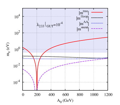
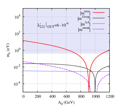
Figure 1: $A_{0}$ dependence of the different contributions to the neutrino mass at the electroweak symmetry breaking scale for our benchmark point BP, with (top) $\lambda_{233}|_{\mathrm{GUT}}=10^{-4}$, (bottom) $\lambda^{\prime}_{222}|_{\rm GUT}=6\cdot 10^{-4}$. Note that only the absolute values of the contributions to the neutrino mass are displayed. The equations for $m_{\nu}^{\textrm{tree}}$ and $m_{\nu}^{\mathbf{\Lambda\Lambda}}$ are given in Eqs. (LABEL:eq:treemass) and (35), respectively. $m_{\nu}^{\textrm{1loop}}$ represents the full one–loop corrections to the neutrino mass, $m_{\nu}^{\textrm{sneut}}$ represents the neutral scalar loops. The grey–shaded area is excluded by the cosmological bound.

As has been noted in Ref. Dreiner:2010ye , there are preferred regions of $B_{3}$ cSSM parameter space in which the neutrino oscillation data can be more easily accommodated. This is illustrated in Fig. 1 for one single LNV coupling. Recall that there is only one tree–level neutrino mass, the second (and third) neutrino mass scale is set by the 1–loop contributions ref:footnote1 . From Fig. 1 (a) [(b)] we see that for a given $\lambda$ [$\lambda^{\prime}$], in the parameter region $100\lesssim A_{0}/{\rm GeV}\lesssim 300$ [$870\lesssim A_{0}/{\rm GeV}\lesssim 930$], the tree–level neutrino mass is sufficiently suppressed relative to the 1–loop neutrino mass to match the mild neutrino mass hierarchy required by the data of maximally 5.7, cf. Eqs. (12), (13). This region of parameter space is determined by the fact that the tree–level neutrino mass (solid cyan line in Fig. 1) has a zero in $A_{0}$ parameter space due to RGE effects. This region exists for every $B_{3}$ cSSM parameter point, provided that

$$A^{(\lambda^{\prime})}_{0} \approx 2\,M_{1/2}$$ (41)

$$A^{(\lambda)}_{0} \approx \frac{M_{1/2}}{2}$$ (42)

for non–zero LNV couplings $\lambda^{\prime}_{ijk}$ or $\lambda_{ijk}$, respectively. Note that the position of the minimum is approximately the same for all indices $i,j,k=1,2,3$. Henceforth we denote the $A_{0}$ minimum with respect to $\lambda$ and $\lambda^{\prime}$ by $A^{(\lambda)}_{0}$ and $A^{(\lambda^{\prime})}_{0}$ respectively. In this paper we focus on this region; more details are given in Sec. IV.2. Therefore we have only 4 $R_{p}$–conserving parameters left, namely $M_{1/2}$, $M_{0}$, ${\rm tan}\beta$ and ${\rm sgn}(\mu)$.

Particles	Masses (GeV)
$\tilde{g}$	1146
$\tilde{\chi}^{\pm}_{1},\tilde{\chi}^{\pm}_{2}$	380	570
$\tilde{\chi}^{0}_{1},\tilde{\chi}^{0}_{2},\tilde{\chi}^{0}_{3},\tilde{\chi}^{0}_{4}$	204	380	552	571
$\tilde{u}_{1},\tilde{c}_{1},\tilde{t}_{1}$	1050	1050	1005
$\tilde{u}_{2},\tilde{c}_{2},\tilde{t}_{2}$	1012	1012	858
$\tilde{d}_{1},\tilde{s}_{1},\tilde{b}_{1}$	1053	1053	971
$\tilde{d}_{2},\tilde{s}_{2},\tilde{b}_{2}$	1008	1008	1002
$\tilde{e}_{1},\tilde{\mu}_{1},\tilde{\tau}_{1}$	353	353	346
$\tilde{e}_{2},\tilde{\mu}_{2},\tilde{\tau}_{2}$	217	217	163
$\tilde{\nu}_{e},\tilde{\nu}_{\mu},\tilde{\nu}_{\tau}$	343	343	331
$h^{0},A^{0},H^{0},H^{\pm}$	112	607	608	612

Table 1: Mass spectrum of the benchmark point BP in the $R_{p}$ conserving limit. From top to bottom, the particles are the gluino, charginos, neutralinos, up–like squarks (2 rows), down–like squarks (2 rows), charged sleptons (2 rows), sneutrinos and the Higgses. The charginos and neutralinos are ordered according to their masses. For a scalar sparticle, a subscript 1(2) denotes that it is primarily ‘left’(‘right’) handed, i.e. the superpartner of a left(right) chiral fermion. This is the convention used in SOFTSUSY. From left to right, the 4 Higgses are the light CP–even Higgs, CP–odd Higgs, heavy CP–even Higgs and the charged Higgs.

For easy comparison with Ref. Dreiner:2010ye , the benchmark point (BP) we use in this paper is chosen to be the same as Ref. Dreiner:2010ye :

$$M_{1/2} = 500\textrm{ GeV}$$

$$M_{0} = 100\textrm{ GeV}$$

$${\rm tan}\beta = 20$$

$${\rm sgn}(\mu) = +1\,.$$ (43)

We have checked that this BP is tachyon–free Allanach:2003eb and that the LEP2 exclusion bound on the light SSM Higgs mass is fulfilled Schael:2006cr ; Barate:2003sz . The spectrum in the $R_{p}$ conserving limit is displayed in Table 1. We see that the squark masses are of order $\mathcal{O}(1\,{\rm TeV})$, whereas the slepton masses are around 200–300 GeV. The lightest supersymmetric particle (LSP) is a stau. However the presence of LNV couplings will render the LSP unstable, making cosmological constraints on the nature of the LSP not applicable Desch:2010gi ; Dreiner:2008rv ; Akeroyd:2001pm .

It should also be pointed out that it is not possible to suppress tree–level contributions for both $\lambda$ and $\lambda^{\prime}$ simultaneously for a universal $A_{0}$ parameter Dreiner:2010ye , as the two minima do not coincide in the $A_{0}$ parameter space, cf. Eqs. (41), (42). Therefore scenarios such as those discussed in Ref. Dey:2008ht , where there is no tree–level neutrino mass at all, are only possible in the $B_{3}$ cSSM if there is only one type of LNV coupling, either $\lambda$ or $\lambda^{\prime}$.

It is also interesting to note that in the case of $\lambda$ couplings [Fig. 1 (a)], the full 1–loop contributions are well approximated by the $\Lambda\Lambda$ loops, whereas in the case of $\lambda^{\prime}$ couplings [Fig. 1 (b)], the approximation is less satisfactory, and further 1–loop contributions such as neutral scalar–neutralino loops also play an important role in parts of the parameter space. However, around the $A^{(\lambda^{\prime})}_{0}$ minimum, the $\Lambda\Lambda$ loops still give a good order of magnitude estimate.

Note that viable neutrino masses could also be obtained away from the $A_{0}$ minimum region by using only off–diagonal LNV couplings, since the tree–level contribution is dominantly generated through diagonal LNV couplings. Thus, scenarios involving only off–diagonal couplings (and up–mixing if using $\lambda^{\prime}$ couplings) also lead to a suppression of the tree–level contribution and could thus potentially reduce the dependence on the $A_{0}$ minimum.

II.6 Low–energy bounds on LNV parameters

Once a set of $\Lambda$ couplings is specified to reproduce the neutrino oscillation data, a natural question arises as to whether the model is compatible with the large number of low energy observables (LEOs). If a considered model predicts LEO values close to current experimental limits, future (non–)observations could (dis–)favor this model.

An extended set of relevant bounds on LEOs is presented in Refs. Barger:1989rk ; Allanach:1999ic ; Barbier:2004ez . Typically these constraints are more important for LNV couplings involving lighter generations. The reasons are two fold: Firstly, the fermion mass term in the loop function $A^{f}_{kn}$ in Eq. (37) implies that, in order to generate a neutrino mass contribution of the same size, LNV couplings involving a light family index $k$ need to be much larger than corresponding couplings with heavy family indices to compensate for the mass suppression. Secondly, experimental constraints generally provide more stringent limits on LNV couplings involving light generations.

In the models presented in later sections, we compare our best fit parameter values with the limits presented in Ref. Barbier:2004ez , as well as a $0\nu\beta\beta$ bound on $\lambda^{\prime}_{111}$ from Ref. Allanach:2009xx . The bounds which are most relevant for the discussion of our results are displayed below:

• ] $\mu\rightarrow eee$ decay:

  $$\lambda_{nij}\lambda_{n11} \lesssim 6.6\cdot 10^{-7}\left(\frac{m_{\tilde{\nu}_{n}}}{100\,{\textrm{G}eV}}\right)^{2},\;\;i,j=12,21$$

  $$\lambda^{\prime}_{211}\lambda^{\prime}_{111} \lesssim 1.3\cdot 10^{-4}\;\text{\cite[cite]{\@@bibref{Authors Phrase1YearPhrase2}{ref:footnote2}{\@@citephrase{(}}{\@@citephrase{)}}}}$$

• ] $\mu-e$ conversion in nuclei:

  $$\lambda_{nij}\lambda^{\prime}_{n11} \lesssim 2.1\cdot 10^{-8}\left(\frac{m_{\tilde{\nu}_{n}}}{100\,{\rm GeV}}\right)^{2},\;\;\;i,j=12,21$$

  $$\lambda^{\prime}_{2n1}\lambda^{\prime}_{1n1} \lesssim 4.3\cdot 10^{-8}\left(\frac{m_{\tilde{q}_{n}}}{100\,{\rm GeV}}\right)^{2},\;\;\;n=2,3$$

  $$\lambda^{\prime}_{21n}\lambda^{\prime}_{11n} \lesssim 4.5\cdot 10^{-8}\left(\frac{m_{\tilde{q}_{n}}}{100\,{\rm GeV}}\right)^{2},\;\;\;n=2,3$$

  $$\lambda^{\prime}_{211}\lambda^{\prime}_{111} \lesssim 4.3\cdot 10^{-8}\cdot\Delta^{-1},$$

  $$\Delta \equiv \left(\frac{100\,{\rm GeV}}{m_{\tilde{u}}}\right)^{2}-\left(\frac{2Z+N}{2N+Z}\frac{100\,{\rm GeV}}{m_{\tilde{d}}}\right)^{2}$$

  For ${}^{48}_{22}$Ti, $(2Z+N)/(2N+Z)=70/74$. This comes from the ratio of the number of valence up–quarks to that of the down–quarks in a nuclei. See Ref. Kim:1997rr .

• ] $\mu$ decay:

  $$\lambda_{12k}\lesssim 0.08\left(\frac{m_{\tilde{e_{kR}}}}{100\,{\rm GeV}}\right)$$

• ] Leptonic $\tau$ decay:

  $$\lambda_{23k},\lambda_{13k}\lesssim 0.08\left(\frac{m_{\tilde{e_{kR}}}}{100\,{\rm GeV}}\right)$$

• ] Forward–backward asymmetry of $Z$ decay:

  $$\lambda_{i3k}(i\neq k\neq 3) \lesssim 0.25\left(\frac{m_{\tilde{\nu}_{\tau}}}{100\,{\rm GeV}}\right)$$

  $$\lambda_{i2k}(i\neq k\neq 2) \lesssim 0.11\left(\frac{m_{\tilde{\nu}_{\mu}}}{100\,{\rm GeV}}\right)$$

• ] Leptonic $K$–meson decay (here $i,j=12,21$):

  $$\lambda_{n11}\lambda^{\prime}_{nij} \lesssim 1.0\cdot 10^{-8}\left(\frac{m_{\tilde{\nu}_{n}}}{100\,{\rm GeV}}\right)^{2},$$

  $$\lambda_{n22}\lambda^{\prime}_{nij} \lesssim 2.2\cdot 10^{-7}\left(\frac{m_{\tilde{\nu}_{n}}}{100\,{\rm GeV}}\right)^{2},$$

  $$\lambda_{n12}\lambda^{\prime}_{nij} \lesssim 6\cdot 10^{-9}\left(\frac{m_{\tilde{\nu}_{n}}}{100\,{\rm GeV}}\right)^{2},$$

  $$\lambda_{n21}\lambda^{\prime}_{nij} \lesssim 6\cdot 10^{-9}\left(\frac{m_{\tilde{\nu}_{n}}}{100\,{\rm GeV}}\right)^{2},$$

• ] $\mu\to e\gamma$:

  $$\lambda_{nl2}\lambda_{nl1} < 8.2\cdot 10^{-5}\cdot$$

  $$\cdot\left[2\left(\frac{\rm 100\,GeV}{m_{\tilde{\nu}_{L}}}\right)^{2}-\left(\frac{\rm 100\,GeV}{m_{\tilde{l}_{L}}}\right)^{2}\right]^{-1}$$

  $$\lambda_{23n}\lambda_{13n} < 2.3\cdot 10^{-4}\cdot$$

  $$\cdot\left[2\left(\frac{\rm 100\,GeV}{m_{\tilde{\nu}_{L}}}\right)^{2}-\left(\frac{\rm 100\,GeV}{m_{\tilde{l}_{R}}}\right)^{2}\right]^{-1}$$

  $$\lambda^{\prime}_{2nl}\lambda^{\prime}_{1nl} < 7.6\cdot 10^{-5}\left(\frac{m_{\tilde{d}_{lR}}}{\rm 100\,GeV}\right)^{2},\;\;n=1,2$$

• ] $0\nu\beta\beta$ (here $\tilde{f}=\tilde{e}_{L},\tilde{u}_{L},\tilde{d}_{R}$):

  $$|\lambda^{\prime}_{111}|\lesssim 5\cdot 10^{-4}\Big{(}\frac{m_{\tilde{f}}}{100\textrm{GeV}}\Big{)}^{2}\Big{(}\frac{m_{{\tilde{g}}/{\tilde{\chi}}}}{100\textrm{GeV}}\Big{)}^{1/2}.$$

These bounds are given in the mass basis, with the reference sparticle mass scale set at 100 GeV. In order to compare our model values with these bounds, we rotate to the mass basis and include the correct mass dependence for all constraints derived from tree–level (4–fermion) operators.

III Choice of LNV parameters

In this section, we choose specific representative scenarios for the LNV sector which will be used for the numerical fit of the neutrino masses and mixings in Sec. IV. First, as a motivation to and a guide line in finding models, we discuss the general neutrino mass matrix in the TBM approximation. As we have seen in Sect. II.1, this is a very good approximation to the data. Later, when performing our numerical fits, we use the experimental values listed in Eqs. (1)–(3). In Sect. III.1 we limit the discussion to “diagonal LNV parameters” $\lambda_{ijj}$ and $\lambda^{\prime}_{ijj}$. In Section III.2 we discuss the more general case which includes “non–diagonal couplings”, i.e. $\lambda_{ijk}$ and $\lambda^{\prime}_{ijk}$ with $j\neq k$.

Since any LNV coupling $\lambda_{ijk},\,\lambda^{\prime}_{ijk}$ could potentially contribute to the effective neutrino mass matrix, we expect a large number of possible solutions to Eqs. (1)–(7). It is well beyond the scope of this paper to attempt to determine them completely. Instead we wish to classify the types of solutions with a potentially minimal set of parameters. We thus make a series of simplifying assumptions, restricting ourselves to a subset of couplings. We will suggest 5 different scenarios (denoted S1 to S5), each making use of LNV coupling combinations from different types ($\lambda$ and $\lambda^{\prime}$) and generations, which we will make explicit as we proceed.

In order to obtain the neutrino mass matrix, we solve the equation

$$U_{TBM}^{\dagger}M^{TBM}_{\nu}U_{TBM}={\rm diag}[m_{\nu\alpha}]\,,$$ (44)

for $M^{TBM}_{\nu}$. Here the neutrino masses $m_{\nu\alpha}(\alpha=1,2,3)$ fit the mass–squared differences and $U_{TBM}$ is given in Eq. (10).

It is natural to split up the resulting neutrino mass matrix into three separate contributions, each of which is proportional to one neutrino mass:

$$M^{TBM}_{\nu} \equiv M_{1}+M_{2}+M_{3}$$ (54)

$$= \frac{m_{\nu 1}}{3}\left(\begin{array}[]{ccc}\phantom{-}2&-1&\phantom{-}1\\ -1&\phantom{-}1/2&-1/2\\ \phantom{-}1&-1/2&\phantom{-}1/2\end{array}\right)+\frac{m_{\nu 2}}{3}\left(\begin{array}[]{ccc}\phantom{-}1&\phantom{-}1&-1\\ \phantom{-}1&\phantom{-}1&-1\\ -1&-1&\phantom{-}1\end{array}\right)+\frac{m_{\nu 3}}{2}\left(\begin{array}[]{ccc}0&0&0\\ 0&1&1\\ 0&1&1\end{array}\right)$$

$$= \frac{1}{6}\left(\begin{array}[]{ccc}4m_{\nu 1}+2m_{\nu 2}&\phantom{4m_{\nu 1}\,\,}2\alpha_{21}\phantom{+\,\,3\alpha_{31}}&\phantom{4m}-2\alpha_{21}\phantom{+\,\,3\alpha_{31}}\\ \phantom{4m_{\nu 1}\,\,}\phantom{-}2\alpha_{21}&m_{\nu 1}+2m_{\nu 2}+3m_{\nu 3}&\phantom{4m}-2\alpha_{21}+3\alpha_{31}\\ \phantom{4m_{\nu 1}}-2\alpha_{21}&\phantom{4m}-2\alpha_{21}+3\alpha_{31}&m_{\nu 1}+2m_{\nu 2}+3m_{\nu 3}\end{array}\right),$$ (58)

where the off–diagonal entries are written in terms of

$$\alpha_{ij} \equiv \frac{\Delta m_{ij}^{2}}{m_{\nu i}+m_{\nu j}}\,.$$ (59)

We observe that all three contributions $M_{\alpha}$ are of the symmetric form

$$(M_{\alpha})_{ij}\propto c^{(\alpha)}_{i}c^{(\alpha)}_{j}\,.$$ (60)

If $U_{TBM}$ is orthogonal, this always follows from Eq. (44), independent of its exact form. The supersymmetric tree–level neutrino mass matrix displays an identical structure if one assigns

$$c^{(tree)}_{i}\sim\lambda^{\prime}_{ijk}(Y_{D})_{jk}\,,$$ (61)

or

$$c^{(tree)}_{i}\sim\lambda_{ijk}(Y_{E})_{jk}\,.$$ (62)

This follows from a first–order approximation of Eq. (LABEL:eq:treelevel), making use of RGE considerations such as Eq. (40) ref:footnote3 . The dominant one–loop level contribution to the neutrino mass matrix does not strictly display the same structure, as can be seen from Eq. (35). However, for diagonal couplings ($j=k$), one can make a similar assignment as in the tree–level case,

$$c^{(loop)}_{j}\sim\lambda^{\prime}_{jkk}(m_{d})_{k}$$ (63)

or

$$c^{(loop)}_{j}\sim\lambda_{jkk}(m_{\ell})_{k}\,,$$ (64)

cf. Eq. (37). We discuss the generalisation to non–diagonal couplings in Sect. III.2.

For simplicity, we mainly focus on solutions which directly reflect the form of Eq. (58) (S1 to S4) ref:footnote6 , namely

$$c_{1}^{(1)}=-2c_{2}^{(1)}=2c_{3}^{(1)}=\sqrt{\frac{2m_{\nu_{1}}}{3}},$$

$$c_{1}^{(2)}=c_{2}^{(2)}=-c_{3}^{(2)}=\sqrt{\frac{m_{\nu 2}}{3}},$$

$$c_{1}^{(3)}=0,\;\;\;c_{2}^{(3)}=c_{3}^{(3)}=\sqrt{\frac{m_{\nu 3}}{2}}\;.$$ (65)

This can minimally be achieved by allowing for exactly one LNV parameter for each coefficient $c_{i}^{(\alpha)}$ ref:footnote5 . The three matrices in Eq. (58) can then be described by 8 coefficients

$$\{c^{(1)}_{1,2,3},\;c^{(2)}_{1,2,3},\;c^{(3)}_{2,3}\}\,,$$ (66)

where we have made use of the fact that $c^{(3)}_{1}=0$ in both the TBM case and the best–fit case, under the assumption that $\theta_{13}=0$. Since we need only two mass scales to describe the neutrino data, we shall assume that the lightest neutrino is massless in the NH and IH cases. Depending on the scenario (NH, IH, DEG), we thus need either five, six or eight non–zero coefficients $c^{(\alpha)}_{i}$.

To illustrate possible alternatives, we show how “non–diagonal” couplings might contribute to neutrino masses in another example (S5).

While we have presented the TBM approximation to display the general coupling structure we are aiming for, in the numerical analysis below we solve Eq. (44) not in the TBM approximation but instead for the best–fit neutrino data given in Eqs. (1)–(7). This results in slightly different values for $c^{(i)}_{j}$. However, the deviation from the TBM case is less than $7\%$ for each $c^{(i)}_{j}$.

III.1 Diagonal LNV scenarios

Scenarios involving only diagonal LNV couplings $\Lambda_{ijk}$ with $j=k$ are the most straightforward to consider. With these we can generate all neutrino mass matrix entries with a minimal set of LNV couplings. The non–diagonal case requires additional couplings, as we discuss below, cf. Sect. III.2. We first discuss normal hierarchy and inverted hierarchy scenarios and then the degenerate case.

• Normal Hierarchy:

  Since the first part of the neutrino mass matrix, $M_{1}$, is zero for NH, we need only five LNV couplings to generate $M_{\nu}\equiv M_{2}+M_{3}$. In order to keep these two contributions $M_{2}$, $M_{3}$ (corresponding to the two non–zero neutrino mass eigenvalues) as independent as possible, we use $\lambda$ couplings for one and $\lambda^{\prime}$ couplings for the other matrix. If we now choose $A_{0}$ such that it lies in the minimum region for either $\lambda$ or $\lambda^{\prime}$ (we denote this by $A_{0}^{(\lambda)}$ and $A_{0}^{(\lambda^{\prime})}$ respectively), cf. Sect. II.5, we can generate one neutrino mass eigenvalue at tree–level and one at loop–level in a nearly independent fashion. This implies that the mass scales can be easily adjusted. We focus on the case $A_{0}^{(\lambda^{\prime})}\sim 2\,M_{1/2}$, where the contribution from $\lambda^{\prime}$ couplings to the tree–level mass matrix is suppressed, because as we will show, for the IH scenarios only this choice of $A_{0}$ is possible. We briefly mention changes for the case $A_{0}^{(\lambda)}\sim M_{1/2}/2$ in NH scenarios during the discussion in Sect. IV D.

  Motivated by the observation that the first row/column of $M_{3}$ is zero (i.e. $c^{(3)}_{1}=0$), and also $\lambda_{111}=0$ due to antisymmetry, we fit

  $$(M_{3})_{ij}\sim\lambda_{i11}\lambda_{j11}\;,$$ (67)

  (i.e. $c^{(3)}_{i}\sim\lambda_{i11}$). We then automatically obtain the structure of $M_{3}$. Because we have chosen $A_{0}^{(\lambda^{\prime})}\sim 2M_{1/2}$, this matrix is dominated by the tree–level contribution. In order to generate $M_{2}$ independently of $M_{3}$ (at one–loop level), we choose

  $$(M_{2})_{ij}\sim\lambda^{\prime}_{ikk}\lambda^{\prime}_{jkk}\;,$$ (68)

  where $k$ is fixed. We present all three cases $k=1,2,3$ in Table 2, denoted S1, S2 and S3, respectively.

  Additionally, we present one further scenario where we depart from the correspondence $c^{(\alpha)}_{i}\sim\Lambda_{i}$. The motivation for this is to consider a neutrino scenario where third generation couplings are dominant, in analogy to the hierarchy of the SM Yukawa couplings. This scenario is particularly interesting because it represents a lower limit on the required size of the LNV couplings under the assumption that no further mechanism exists to contribute to the neutrino masses. We discuss this aspect in more detail in section V. In order to be able to fit the matrices $M_{2}$, $M_{3}$ only with third generation couplings $\lambda_{i33}$ and $\lambda^{\prime}_{i33}$, one of those matrices needs to fulfill $(M_{i})_{3k}=0$ due to the antisymmetry of $\lambda$ in the first two indices. To achieve this, we build a suitable superposition of the matrices $M_{2}$ and $M_{3}$. We denote the new coefficients by $\tilde{c}^{(\alpha)}_{i}$ in S4 of Table 2.

• Inverse Hierarchy:

  As mentioned in the case of Normal Hierarchy, $\lambda_{ijj}$ couplings will always lead to one row/column of zeros in the generated neutrino mass matrix. Since in the case of Inverse Hierarchy, the two non–zero matrices $M_{1}$ and $M_{2}$ are both non–zero in all entries, we take this as motivation to fit $M_{1}$ and $M_{2}$ with $\lambda^{\prime}$ couplings only (however, for completeness we also present one scenario with both $\lambda$ and $\lambda^{\prime}$ couplings, cf. next paragraph). With only $\lambda^{\prime}$ couplings present, we set the value of $A_{0}$ to $A_{0}^{(\lambda^{\prime})}\sim 2\,M_{1/2}$, such that all tree–level contributions are suppressed, and the two mass scales are both generated at loop level. Otherwise the neutrino mass hierarchy would be much larger than experimentally observed, cf. Sec. II.5. We display the three possibilities arising from

  $$(M_{1})_{ij} \sim \lambda^{\prime}_{ikk}\lambda^{\prime}_{jkk}\,,$$ (69)

  $$(M_{2})_{ij} \sim \lambda^{\prime}_{ill}\lambda^{\prime}_{jll}\,,$$ (70)

  where $l<k$ ref:footnote7 in Table 2. These models are labelled (IH) S1, S2 and S3.

  If we choose $\lambda_{i\ell\ell}$ couplings instead of $\lambda^{\prime}_{i\ell\ell}$ in Eq. (70), this would again generate a (unwanted) row/column of zeros in $M_{2}$. Therefore, in this case we need to combine, for example, $\lambda_{i33}$ with $\lambda_{322}$ in order to generate non–zero entries for the third row/column of $M_{2}$. Such a combination of couplings generates a matrix of the form $c^{(2)}_{i}c^{(2)}_{j}$, where $c^{(2)}_{1,2}$ and $c^{(2)}_{3}$ originate from $\lambda_{i33}$ and $\lambda_{322}$ at tree–level respectively, because these couplings generate $\kappa_{i}$ via the RGEs, cf. Eqs. (LABEL:eq:treelevel) and (40). In order to ensure that $M_{2}$ is generated at tree–level, we still set $A_{0}^{(\lambda^{\prime})}=2M_{1/2}$, such that we are able to fit Eq. (58). This case is also listed under S4 in Table 2.

• Degenerate Masses:

  Since for degenerate masses, all three matrices $M_{1,2,3}$ are non–zero and of similar magnitude, this scenario is a combination of choices made for NH and IH. As explained for the case of NH, we choose

  $$(M_{3})_{ij}\sim\lambda_{i11}\lambda_{j11}\;.$$ (71)

  To generate $M_{1}$ and $M_{2}$, we fit in analogy to the IH case

  $$(M_{1})_{ij}\sim\lambda^{\prime}_{ikk}\lambda^{\prime}_{jkk}$$ (72)

  $$(M_{2})_{ij}\sim\lambda^{\prime}_{ill}\lambda^{\prime}_{jll}\;.$$ (73)

  These models are listed in Table 2 as (DEG) S1, S2 and S3. Here, as in the IH case, only the parameter choice $A_{0}^{(\lambda^{\prime})}$ is possible in order to suppress the $\lambda^{\prime}$ contribution to the tree–level neutrino mass.

	Normal Hierarchy (NH)	Inverse Hierarchy (IH)	Degenerate (DEG)
S1	$c^{(1)}_{i}\sim 0$	$c^{(1)}_{i}\sim\lambda^{\prime}_{i11}$	$c^{(1)}_{i}\sim\lambda^{\prime}_{i11}$
	$c^{(2)}_{i}\sim\lambda^{\prime}_{i11}$	$c^{(2)}_{i}\sim\lambda^{\prime}_{i22}$	$c^{(2)}_{i}\sim\lambda^{\prime}_{i22}$
	$c^{(3)}_{i}\sim\lambda_{i11}$	$c^{(3)}_{i}\sim 0$	$c^{(3)}_{i}\sim\lambda_{i11}$
S2	$c^{(1)}_{i}\sim 0$	$c^{(1)}_{i}\sim\lambda^{\prime}_{i11}$	$c^{(1)}_{i}\sim\lambda^{\prime}_{i11}$
	$c^{(2)}_{i}\sim\lambda^{\prime}_{i22}$	$c^{(2)}_{i}\sim\lambda^{\prime}_{i33}$	$c^{(2)}_{i}\sim\lambda^{\prime}_{i33}$
	$c^{(3)}_{i}\sim\lambda_{i11}$	$c^{(3)}_{i}\sim 0$	$c^{(3)}_{i}\sim\lambda_{i11}$
S3	$c^{(1)}_{i}\sim 0$	$c^{(1)}_{i}\sim\lambda^{\prime}_{i22}$	$c^{(1)}_{i}\sim\lambda^{\prime}_{i22}$
	$c^{(2)}_{i}\sim\lambda^{\prime}_{i33}$	$c^{(2)}_{i}\sim\lambda^{\prime}_{i33}$	$c^{(2)}_{i}\sim\lambda^{\prime}_{i33}$
	$c^{(3)}_{i}\sim\lambda_{i11}$	$c^{(3)}_{i}\sim 0$	$c^{(3)}_{i}\sim\lambda_{i11}$
S4	$c^{(1)}_{i}\sim 0$	$c^{(1)}_{i}\sim\lambda^{\prime}_{i33}$
	$\tilde{c}^{(2)}_{i}\sim\lambda^{\prime}_{i33}$	$c^{(2)}_{i}\sim\lambda_{i33}\;\&\;\lambda_{322}$	–
	$\tilde{c}^{(3)}_{i}\sim\lambda_{i33}$	$c^{(3)}_{i}\sim 0$
S5	$c^{(1)}_{i}\sim 0$		$c^{(1)}_{i}\sim\lambda^{\prime}_{i33}$
	$c^{(2)}_{i}\sim\lambda^{\prime}_{i23}\;\&\;\lambda^{\prime}_{i32}$	–	$c^{(2)}_{i}\sim\lambda_{i33}\;\&\;\lambda_{322}$
	$c^{(3)}_{i}\sim\lambda_{i11}$		$c^{(3)}_{i}\sim\lambda_{231}\;\&\;\lambda_{213}\;\&\;\lambda_{312}\;(\&\;\lambda_{313})$

Table 2: Overview of the “diagonal” (S1 – S4) and “non–diagonal” (S5) scenarios used for our numerical analysis.

III.2 Non–diagonal LNV scenarios

In this section, we depart from the diagonal coupling scenarios and discuss the effects of introducing “non–diagonal” couplings.

When allowing for non–diagonal LNV couplings $\lambda^{\prime}_{ikl}$ ($\lambda_{ikl}$), $l\neq k$, we generally need more couplings than in the diagonal case. This is because at one–loop level ref:footnote8 , neutrino masses are dominantly generated proportional to $\lambda^{\prime}_{ikl}\lambda^{\prime}_{ilk}$ ($\lambda_{ikl}\lambda_{ilk}$). Thus, the assignment of one LNV coupling to one $c^{(\alpha)}_{i}$ parameter (Eq. (60)) is not possible for the part of the neutrino mass matrix generated at 1–loop level. Instead, we require

$$c^{(\alpha)}_{i}c^{(\alpha)}_{j}\sim\frac{1}{2}\cdot(\lambda^{\prime}_{ikl}\lambda^{\prime}_{jlk}+\lambda^{\prime}_{ilk}\lambda^{\prime}_{jkl})\;(m_{d})_{k}\;(m_{d})_{l}$$ (74)

where $k$, $l$ are fix (similarly for $\lambda$ couplings). This effectively doubles the number of LNV parameters if we choose $k\neq l$. Phenomenologically, one can distinguish between two cases:

• $\lambda^{\prime}_{ikl}\approx\lambda^{\prime}_{ilk}$ (same order of magnitude)

• $\lambda^{\prime}_{ikl}\gg\lambda^{\prime}_{ilk}$ or vice versa (strong hierarchy)

In the first case (a), the size of the couplings will not differ significantly from the diagonal case. For illustrative purposes, we will present numerical results for a non–diagonal scenario similar to the S3 NH example, which we list under S5 NH in Table 2. Here, we take as starting values $\lambda^{\prime}_{i23}=\lambda^{\prime}_{i32}$ and thus, a simplified form of Eq. (74) is $c^{(2)}_{i}\sim\lambda^{\prime}_{i32}$, similar to the assignment in the diagonal case.

In the latter case (b), the size of the couplings become very different from those in the diagonal scenarios. In particular, some of the couplings can become very large. This is potentially of great interest experimentally. However, various low–energy bounds could potentially be violated. This can be illustrated with the help of the following example with degenerate neutrino masses, which we list under S5 DEG in Table 2. Here, the first two neutrino masses are generated as in the case of S4 IH (however, now for normal mass ordering): $M_{2}$ is generated at tree–level via diagonal $\lambda_{i33}$ and $\lambda_{322}$ couplings, and $M_{1}$ is generated at loop–level via $\lambda^{\prime}_{i33}$ couplings. However, now we additionally generate $M_{3}$ at one–loop level via the 3 off–diagonal $\lambda$ couplings $\lambda_{231}$, $\lambda_{213}$ and $\lambda_{312}$. The latter do not lead to tree–level neutrino masses because the leptonic Higgs–Yukawa coupling is (nearly) diagonal and thus the tree–level generating term $\lambda_{ijk}(Y_{E})_{jk}$ is (practically) zero. As we will see, the benchmark point we use leads to a very large $\lambda_{231}$ beyond the perturbativity limit. For this reason, a different BP point, labelled as BP2, will be introduced for this scenario in Sect. V.2 ref:footnote15 .

To obtain a qualitative understanding of the relative size of the couplings, first note that $\lambda_{133}$ contributes to both $M_{2}$ and $M_{3}$ due to the antisymmetry, $\lambda_{133}\equiv-\lambda_{313}$. We choose the $A_{0}^{(\lambda^{\prime})}$ minimum, and thus generate $M_{2}$ at tree level. The value of $\lambda_{133}$ is therefore fixed, and is forced to be small due to its coupling with the large tau Yukawa coupling $(Y_{E})_{33}$. The matrices $M_{1}$ and $M_{3}$ are then generated at loop level. The coupling product $\lambda_{231}\lambda_{313}=-\lambda_{231}\lambda_{133}$ is responsible for generating $(M_{3})_{23}$. This implies that $\lambda_{231}$ needs to be large in order to compensate for the smallness of $\lambda_{313}$. When now fitting $(M_{3})_{22}\sim\lambda_{231}\lambda_{213}$, the large $\lambda_{231}$ then leads to a hierarchically smaller $\lambda_{213}$ in order to be consistent with the experimental result. Similarly, $\lambda_{231}$ leads to a small $\lambda_{312}$ by their contribution to $(M_{3})_{33}$ via $\lambda_{312}\lambda_{321}(A^{l}_{12}+A^{l}_{21})$ as shown in Eq. (35).

IV Numerical Analysis

In this section, we present the numerical results. We will first discuss the relevant aspects of SOFTSUSYv3.1.5 for our analysis. We then describe our minimization procedure. Next we present our best–fit solutions for the normal hierarchy, inverted hierarchy and the degenerate case, respectively. In the last subsection we discuss these results.

IV.1 Preliminaries

Our numerical simulation is performed using an adaptation of SOFTSUSYv3.1.5 , which will be made public in the near future. Until then, we refer interested readers to the SOFTSUSY  manual Allanach:2009bv for the detailed procedure of obtaining the $B_{3}$ SSM mass spectrum. We use the program package MINUIT2  and a Markov chain Monte Carlo method (Metropolis–Hastings algorithm) for fitting the LNV couplings $\Lambda_{ijk}$ to the neutrino data.

We now comment briefly on the additional features we include in SOFTSUSY  and the determination of the $U_{\rm PMNS}$ mixing in the following. Our calculation improves on SOFTSUSYv3.1.5 by including the one–loop contributions to the neutrino–neutralino mass matrix, as well as all ${{\not\!{R}}_{p}}$ tadpole corrections to the Higgs and sneutrino VEVs. Because the superfields $L_{i}$ and $H_{d}$ have the same quantum numbers, we organize the computation to treat these fields on equal footing. To ensure the accuracy, an independent calculation was performed without using this symmetry. We have also checked that in the $R_{p}$ conserving limit our results agree with the internal results in SOFTSUSYv3.1.5.

The ${{\not\!{R}}_{p}}$ tadpole corrections are included in the SOFTSUSY iteration procedure which minimizes the 5–dimensional EW symmetry breaking neutral scalar potential. The effective 3 $\times$ 3 neutrino mass matrix $\mathcal{M}_{\nu}^{{\rm eff}}$ and the effective neutrino mixing matrix $U_{\nu}$ are calculated at the EWSB scale given an input set of LNV parameters at the unification scale. Note that within SOFTSUSY , the condition that the charged lepton mixing matrix is diagonal is imposed at the electroweak scale. Thus, $U_{\rm PMNS}=U_{\nu}$ ref:footnote10 .

IV.2 Minimization Procedure

Our goal is to find numerical values for each LNV scenario specified in Table 2, such that we obtain the experimentally observed neutrino data, Eqs. (1)–(7), at the 1$\,\sigma$ level by means of least–square fitting. In order to achieve this also in degenerate scenarios, which necessarily involve some fine–tuning (as we discuss in Sect. V), we use a multistep procedure as outlined below.

We take as initial values for each set of LNV parameters at the unification scale $M_{X}$

$$\Lambda_{ikk}\sim c^{(\alpha)}_{i}\frac{1}{{(Y_{f})_{kk}}}$$ (75)

(no summation over $k$) as specified in Table 2. $f$ denotes a down quark for a $\lambda^{\prime}$ and a charged lepton for a $\lambda$ coupling. The proportionality factor is estimated from the upper bound on the LNV couplings which comes from the upper bound on the neutrino mass from WMAP measurements, cf. Ref. Dreiner:2010ye .

Next, we perform a pre–iteration within our modified version of SOFTSUSY, where we make the simplifying assumption that the generation of the tree–level (by $\Lambda=\lambda$) and 1–loop level (by $\Lambda=\lambda^{\prime}$) neutrino mass matrices $M_{\alpha}$ in Eq.  (58) are independent of each other. So for each $M_{\alpha}$ we separately fit the relevant $\Lambda_{ijk}$. In our iteration procedure we set

$$\Lambda_{ijk}|_{new}=\sqrt{\frac{(M_{\alpha}^{obs})_{ii}}{(M_{\alpha}^{softsusy})_{ii}}}\Lambda_{ijk}|_{old}\,.$$ (76)

Here $M_{\alpha}^{softsusy}$ is the effective neutrino mass matrix (at 1–loop level) obtained via the seesaw–mechanism with SOFTSUSY . In the first step we use the initial values corresponding to Eq. (75). We obtain $(M_{\alpha}^{obs})_{ii}$ by inverting Eq. (44), without using the TBM approximation. For $m_{\nu\alpha}$ we use the experimental best–fit values. And for the diagonalization matrix $U$, we implement the general form, using $\theta_{12},\,\theta_{23}$ from the experimental best–fit, as well as $\theta_{13}=0$. In Eq. (76) there is also no sum over $i$.

This gives a very good order of magnitude estimate for all LNV couplings and thus a suitable starting point for our least–square fit. However, so far each set of couplings $\Lambda_{ijk}\sim c^{(\alpha)}_{i}/(Y_{f})_{kk}$ has only been fit separately for each $\alpha$, while keeping the other LNV couplings equal to zero. When fitting all LNV couplings simultaneously, they can affect each other via the RGEs and through contributions to the other $M_{\alpha}^{obs}$. Note that these effects are easily controllable for NH and IH scenarios. However, in the case of DEG scenarios, some strong cancellations occur for some entries of the effective neutrino mass matrix, e.g. the $(M_{\nu})_{13}=(M_{1})_{13}+(M_{2})_{13}$ entry in Eq. (58). Here, both individual entries $(M_{\alpha})_{13}$ are of the order of the generated neutrino mass, but the resulting $(M_{\nu})_{13}$ entry is at least 3 orders of magnitude smaller. This will become relevant in the next step of our procedure.

After these first approximations, we next fit all LNV parameters specified for each scenario in Table 2 simultaneously. We calculate the full $7\times 7$ neutralino–neutrino mass matrix with SOFTSUSY. The $3\times 3$ neutrino mass matrix is then obtained via the seesaw mechanism, and is used in order to extract predictions for the neutrino masses and mixing angles.

We define a $\chi^{2}$ function

$$\chi^{2}\equiv\frac{1}{N_{obs}}\sum_{i=1}^{N_{obs}}\left(\frac{f^{softsusy}_{i}-f^{obs}_{i}}{\delta_{i}}\right)^{2}$$ (77)

where $f_{i}^{obs}$ are the central values of the $N_{obs}$ experimental observables defined in Eqs. (1)–(7), $f_{i}^{softsusy}$ are the corresponding numerical predictions and $\delta_{i}$ are the 1$\,\sigma$ experimental uncertainties. We minimize Eq. (77) with a stepping method of the program package MINUIT2 for the NH/IH case. In the DEG scenarios, MINUIT2 initially does not converge due to the points made in the last paragraph. Therefore, we first use the Hastings–Metropolis algorithm to obtain a $\chi^{2}<\mathcal{O}(10)$. Subsequently, the same MINUIT2 routine as in the NH/IH case is used. We accept a minimization result as successful if our minimization procedure yields $\chi^{2}<1$.

Simultaneously, we ensure that the conditions

$$\sum_{i}m_{\nu_{i}}\lesssim 0.4\textrm{ eV}$$

$$\sin^{2}(\theta_{13})<0.047$$ (78)

are fulfilled.

V Discussion of Results

	Normal Hierarchy	Inverse Hierarchy	Degenerate
S1		$\lambda^{\prime}_{111}=\>\>\>\,\mathbf{3.94\cdot 10^{-2}}$ [b1],[b2],[b8]	$\lambda^{\prime}_{111}=\>\>\>\,\mathbf{5.85\cdot 10^{-2}}$ [b1],[b2],[b7],[b8]
		$\lambda^{\prime}_{211}=\mathbf{-1.88\cdot 10^{-2}}$ [b1],[b2]	$\lambda^{\prime}_{211}=\mathbf{-3.63\cdot 10^{-2}}$ [b1],[b2],[b6],[b7]
		$\lambda^{\prime}_{311}=\>\>\>\,1.94\cdot 10^{-2}$	$\lambda^{\prime}_{311}=\>\>\>\,\mathbf{3.35\cdot 10^{-2}}$ [b6]
	$\lambda^{\prime}_{111}=\>\>\>\,\mathbf{1.12\cdot 10^{-2}}$ [b2],[b8]	$\lambda^{\prime}_{122}=\>\>\>\,1.21\cdot 10^{-3}$	$\lambda^{\prime}_{122}=\>\>\>\,2.18\cdot 10^{-3}$
	$\lambda^{\prime}_{211}=\>\>\>\,\mathbf{8.76\cdot 10^{-3}}$	$\lambda^{\prime}_{222}=\>\>\>\,1.27\cdot 10^{-3}$	$\lambda^{\prime}_{222}=\>\>\>\,1.63\cdot 10^{-3}$
	$\lambda^{\prime}_{311}=-1.48\cdot 10^{-2}$	$\lambda^{\prime}_{322}=-1.31\cdot 10^{-3}$	$\lambda^{\prime}_{322}=-2.09\cdot 10^{-3}$
	$\lambda_{211}=\>\>\>\,\mathbf{1.52\cdot 10^{-2}}$ [b2]		$\lambda_{211}=\>\>\>\,\mathbf{2.55\cdot 10^{-2}}$ [b2],[b6]
	$\lambda_{311}=\>\>\>\,1.37\cdot 10^{-2}$		$\lambda_{311}=\>\>\>\,\mathbf{2.28\cdot 10^{-2}}$ [b6]
S2		$\lambda^{\prime}_{111}=\>\>\>\,\mathbf{3.99\cdot 10^{-2}}$ [b1],[b2],[b8]	$\lambda^{\prime}_{111}=\>\>\>\,\mathbf{6.87\cdot 10^{-2}}$ [b1],[b2],[b7],[b8]
		$\lambda^{\prime}_{211}=\mathbf{-1.81\cdot 10^{-2}}$ [b1],[b2]	$\lambda^{\prime}_{211}=\mathbf{-2.90\cdot 10^{-2}}$ [b1],[b2],[b6],[b7]
		$\lambda^{\prime}_{311}=\>\>\>\,1.89\cdot 10^{-2}$	$\lambda^{\prime}_{311}=\>\>\>\,\mathbf{3.18\cdot 10^{-2}}$ [b6]
	$\lambda^{\prime}_{122}=\>\>\>\,5.08\cdot 10^{-4}$	$\lambda^{\prime}_{133}=\>\>\>\,3.09\cdot 10^{-5}$	$\lambda^{\prime}_{133}=\>\>\>\,4.99\cdot 10^{-5}$
	$\lambda^{\prime}_{222}=\>\>\>\,3.88\cdot 10^{-4}$	$\lambda^{\prime}_{233}=\>\>\>\,3.21\cdot 10^{-5}$	$\lambda^{\prime}_{233}=\>\>\>\,2.98\cdot 10^{-5}$
	$\lambda^{\prime}_{322}=-6.97\cdot 10^{-4}$	$\lambda^{\prime}_{333}=-3.35\cdot 10^{-5}$	$\lambda^{\prime}_{333}=-7.43\cdot 10^{-5}$
	$\lambda_{211}=\>\>\>\,1.52\cdot 10^{-2}$		$\lambda_{211}=\>\>\>\,\mathbf{2.99\cdot 10^{-2}}$ [b2],[b6]
	$\lambda_{311}=\>\>\>\,1.37\cdot 10^{-2}$		$\lambda_{311}=\>\>\>\,\mathbf{2.10\cdot 10^{-2}}$ [b6]
S3		$\lambda^{\prime}_{122}=\>\>\>\,1.80\cdot 10^{-3}$	$\lambda^{\prime}_{122}=\>\>\>\,2.93\cdot 10^{-3}$
		$\lambda^{\prime}_{222}=-8.29\cdot 10^{-4}$	$\lambda^{\prime}_{222}=-1.98\cdot 10^{-3}$
		$\lambda^{\prime}_{322}=\>\>\>\,8.64\cdot 10^{-4}$	$\lambda^{\prime}_{322}=\>\>\>\,5.79\cdot 10^{-4}$
	$\lambda^{\prime}_{133}=\>\>\>\,1.30\cdot 10^{-5}$	$\lambda^{\prime}_{133}=\>\>\>\,3.11\cdot 10^{-5}$	$\lambda^{\prime}_{133}=\>\>\>\,5.18\cdot 10^{-5}$
	$\lambda^{\prime}_{233}=\>\>\>\,4.84\cdot 10^{-6}$	$\lambda^{\prime}_{233}=\>\>\>\,3.22\cdot 10^{-5}$	$\lambda^{\prime}_{233}=\>\>\>\,5.78\cdot 10^{-5}$
	$\lambda^{\prime}_{333}=-2.28\cdot 10^{-5}$	$\lambda^{\prime}_{333}=-3.32\cdot 10^{-5}$	$\lambda^{\prime}_{333}=-5.13\cdot 10^{-5}$
	$\lambda_{211}=\>\>\>\,1.55\cdot 10^{-2}$		$\lambda_{211}=\>\>\>\,1.71\cdot 10^{-2}$
	$\lambda_{311}=\>\>\>\,1.40\cdot 10^{-2}$		$\lambda_{311}=\>\>\>\,3.08\cdot 10^{-2}$
S4	$\lambda^{\prime}_{133}=-6.80\cdot 10^{-6}$	$\lambda^{\prime}_{133}=\>\>\>\,3.96\cdot 10^{-5}$
	$\lambda^{\prime}_{233}=\>\>\>\,2.81\cdot 10^{-5}$	$\lambda^{\prime}_{233}=-2.81\cdot 10^{-5}$
	$\lambda^{\prime}_{333}=\>\>\>\,4.21\cdot 10^{-5}$	$\lambda^{\prime}_{333}=\>\>\>\,2.89\cdot 10^{-5}$
	$\lambda_{133}=\>\>\>\,1.32\cdot 10^{-6}$	$\lambda_{133}=\>\>\>\,3.23\cdot 10^{-6}$
	$\lambda_{233}=\>\>\>\,2.70\cdot 10^{-6}$	$\lambda_{233}=\>\>\>\,3.48\cdot 10^{-6}$
		$\lambda_{322}=-5.64\cdot 10^{-5}$
S5	$\lambda^{\prime}_{123}=\>\>\>\,5.76\cdot 10^{-5}$		$\lambda^{\prime}_{133}=-3.11\cdot 10^{-5}$
	$\lambda^{\prime}_{132}=\>\>\>\,5.75\cdot 10^{-5}$		$\lambda^{\prime}_{233}=\>\>\>\,8.79\cdot 10^{-5}$
	$\lambda^{\prime}_{223}=\>\>\>\,6.23\cdot 10^{-5}$		$\lambda^{\prime}_{333}=-4.14\cdot 10^{-5}$
	$\lambda^{\prime}_{232}=\>\>\>\,6.24\cdot 10^{-5}$		$\lambda_{133}=\>\>\>\,1.99\cdot 10^{-6}$
	$\lambda^{\prime}_{323}=-5.88\cdot 10^{-5}$		$\lambda_{233}=\>\>\>\,4.08\cdot 10^{-6}$
	$\lambda^{\prime}_{332}=-6.00\cdot 10^{-5}$		$\lambda_{322}=-2.57\cdot 10^{-5}$
	$\lambda_{211}=\>\>\>\,1.52\cdot 10^{-2}$		$\lambda_{231}=-5.67\cdot 10^{-2}$
	$\lambda_{311}=\>\>\>\,1.39\cdot 10^{-2}$		$\lambda_{213}=-2.03\cdot 10^{-5}$
			$\lambda_{312}=\>\>\>\,2.54\cdot 10^{-3}$

Table 3: Best–fit points for the LNV parameters at the unification scale $M_{X}$ for our benchmark point BP and $A_{0}^{(\lambda^{\prime})}=912.3$ GeV, except for S5 DEG, where BP2 and $A_{0}^{(\lambda^{\prime})}=1059.2$ GeV are used, cf. Sect. V.2. The couplings printed in bold violate one of the low–energy bounds [b1]–[b7] which are listed in Sect. II.6. Note that the values are given at 2 significance level only for better readability. In order to reproduce the results, higher significance is needed as is clear from Eq. (80). Readers are encouraged to contact the authors to obtain the exact values.

	Normal Hierarchy							Inverse Hierarchy							Degenerate
Data								$c^{(1)}_{1}:$	$c^{(1)}_{2}:$	$c^{(1)}_{3}$	=	2.09 :	$-$0.98 :	1	$c^{(1)}_{1}:$	$c^{(1)}_{2}:$	$c^{(1)}_{3}$	=	2.09 :	$-$0.98 :	1
	$c^{(2)}_{1}:$	$c^{(2)}_{2}:$	$c^{(2)}_{3}$	=	0.94 :	0.99 :	$-$1	$c^{(2)}_{1}:$	$c^{(2)}_{2}:$	$c^{(2)}_{3}$	=	0.94 :	0.99 :	$-$1	$c^{(2)}_{1}:$	$c^{(2)}_{2}:$	$c^{(2)}_{3}$	=	0.94 :	0.99 :	$-$1
		$c^{(3)}_{2}:$	$c^{(3)}_{3}$	=		0.99 :	1									$c^{(3)}_{2}:$	$c^{(3)}_{3}$	=		0.99 :	1
S1								$\lambda^{\prime}_{111}:$	$\lambda^{\prime}_{211}:$	$\lambda^{\prime}_{311}$	=	2.04 :	$-$0.97 :	1	$\lambda^{\prime}_{111}:$	$\lambda^{\prime}_{211}:$	$\lambda^{\prime}_{311}$	=	1.75 :	$-$1.09 :	1
	$\lambda^{\prime}_{111}:$	$\lambda^{\prime}_{211}:$	$\lambda^{\prime}_{311}$	=	0.75 :	0.59 :	$-$1	$\lambda^{\prime}_{122}:$	$\lambda^{\prime}_{222}:$	$\lambda^{\prime}_{322}$	=	0.93 :	0.97 :	$-$1	$\lambda^{\prime}_{111}:$	$\lambda^{\prime}_{211}:$	$\lambda^{\prime}_{311}$	=	1.04 :	0.78 :	$-$1
		$\lambda_{211}:$	$\lambda_{311}$	=		1.11 :	1									$\lambda_{211}:$	$\lambda_{311}$	=		1.19 :	1
S2								$\lambda^{\prime}_{111}:$	$\lambda^{\prime}_{211}:$	$\lambda^{\prime}_{311}$	=	2.12 :	$-$0.96 :	1	$\lambda^{\prime}_{111}:$	$\lambda^{\prime}_{211}:$	$\lambda^{\prime}_{311}$	=	2.11 :	$-$0.91 :	1
	$\lambda^{\prime}_{122}:$	$\lambda^{\prime}_{222}:$	$\lambda^{\prime}_{322}$	=	0.73 :	0.56 :	$-$1	$\lambda^{\prime}_{133}:$	$\lambda^{\prime}_{233}:$	$\lambda^{\prime}_{333}$	=	0.93 :	0.96 :	$-$1	$\lambda^{\prime}_{133}:$	$\lambda^{\prime}_{233}:$	$\lambda^{\prime}_{333}$	=	0.67 :	0.40 :	$-$1
		$\lambda_{211}:$	$\lambda_{311}$	=		1.11 :	1									$\lambda_{211}:$	$\lambda_{311}$	=		1.42 :	1
S3								$\lambda^{\prime}_{122}:$	$\lambda^{\prime}_{222}:$	$\lambda^{\prime}_{322}$	=	2.09 :	$-$0.96 :	1	$\lambda^{\prime}_{122}:$	$\lambda^{\prime}_{222}:$	$\lambda^{\prime}_{322}$	=	5.06 :	$-$3.41 :	1
	$\lambda^{\prime}_{133}:$	$\lambda^{\prime}_{233}:$	$\lambda^{\prime}_{333}$	=	0.57 :	0.21 :	$-$1	$\lambda^{\prime}_{133}:$	$\lambda^{\prime}_{233}:$	$\lambda^{\prime}_{333}$	=	0.93 :	0.97 :	$-$1	$\lambda^{\prime}_{133}:$	$\lambda^{\prime}_{233}:$	$\lambda^{\prime}_{333}$	=	1.01 :	1.13 :	$-$1
		$\lambda_{211}:$	$\lambda_{311}$	=		1.11 :	1									$\lambda_{211}:$	$\lambda_{311}$	=		0.56 :	1

Table 4: Ratios of the LNV parameters at the unification scale $M_{X}$ for scenarios S1, S2 and S3 and the ratios $c^{(\alpha)}_{1}:c^{(\alpha)}_{2}:c^{(\alpha)}_{3}$ inferred from experimental data. For comparison, the ratios $c^{(\alpha)}_{1}:c^{(\alpha)}_{2}:c^{(\alpha)}_{3}$ in the TBM limit are $(2:-1:1)$, $(1:1:-1)$ and $(0:1:1)$ for $\alpha=1,2$ and $3$ respectively.

We present our numerical results in Table 3. In the three columns, we show our best–fit solutions for normal hierarchy, inverse hierarchy and degenerate masses, respectively. In the five rows, we show our solutions for the various scenarios enlisted in Table 2. S1–S4 are the “diagonal” LNV scenarios, while S5 involves non–diagonal couplings, as discussed in the previous section. In order to illustrate the low energy bounds most relevant to our scenarios, we also display models which do not satisfy all constraints. These solutions are highlighted in bold and the violated bound(s) are also stated.

V.1 Diagonal LNV Scenarios

We first discuss some general features of the best fit parameter sets. Focusing on the three scenarios S1–S3, some ratios among the LNV couplings are displayed in Table 4. We see that the results reflect the basic structure of our ansätz Eq. (75). In particular, the relative signs among different LNV couplings are reproduced. However, the relative magnitude among the couplings are expected to deviate somewhat from Eqs. (75) and  (65). One reason is that our LNV couplings should mirror the structure of Eq. (65) at the electroweak scale, while in Table 3 and Table 4 the couplings are given at the unification scale. So RG running needs to be taken into account. However the change in the LNV couplings when going to the unification scale is not uniform for all couplings. Also, we fit the oscillation data given in Sec. I instead of the TBM approximation, such that the $c_{i}^{(\alpha)}$ differ from Eq. (65) already by up to $7\%$ percent.

We also see from Table 4 that the LNV parameters in the IH scenarios follow the pattern of $c_{i}^{(\alpha)}$ more closely than those in the NH and DEG scenarios. For the IH scenarios, the tree level contribution is suppressed by choosing $A_{0}$ appropriately. The neutrino mass matrix entries are dominated by loop contributions and the associated couplings should then reflect the near TBM structure as well as the orthogonality of the vectors $c^{(\alpha)}$. However for the NH and DEG scenarios, the significant contributions from both tree and loop masses mean that while the $c_{i}^{(\alpha)}$ have the expected ratios for each $\alpha$ after pre–iteration, once contributions from different $\alpha$’s are combined for the full iteration they interfere with each other. For example, the presence of $\lambda$ couplings changes the position of the $A_{0}^{(\lambda^{\prime})}$ minimum, making the contributions of the $\lambda^{\prime}$ couplings to the tree level masses less suppressed, thus leading to the larger deviation.

It is clear from Eq. (75) that the magnitude of diagonal LNV couplings should decrease from first to third generation (while generating the same neutrino masses), because the LNV couplings have to balance out the effect of the Higgs–Yukawa–couplings, which increase with generation. For example, comparing the size of $\lambda^{\prime}_{ikk}$ in scenarios S1–S3 in the IH case, one observes that the difference in magnitude of the LNV couplings mirrors the hierarchy of down–type quark masses, $\lambda^{\prime}_{ijj}/\lambda^{\prime}_{ikk}\sim(m_{d})_{k}/(m_{d})_{j}$ for fixed index $i$.

As we see in Table 3, models involving first generation couplings ($\lambda^{\prime}_{111}$ and $\lambda^{\prime}_{211}$) are disfavored due to strong constraints from $\mu\rightarrow eee$ [b1], $\mu$–$e$ conversions [b2] and $0\nu\beta\beta$ [b8]. In addition, the $\lambda_{211}$ in S1 NH, S1 DEG and S2 DEG violate the two–coupling bound from $\mu$–$e$ conversion [b2] in conjunction with the large $\lambda^{\prime}_{111}$ coupling. Limits on leptonic K–meson decay [b6] and $\mu\to e\gamma$ [b7] are also seen to be violated in degenerate scenarios S1 DEG and S2 DEG involving diagonal first generation couplings. The second generation LNV Yukawa couplings are of the order of $10^{-3}$ ($10^{-4}$) for IH and DEG (NH) scenarios ref:footnote9 and safely satisfy all low–energy bounds. The third generation couplings take on values between $10^{-5}$ and $10^{-6}$.

Collider implications of the solutions we obtained will be discussed in section VI. Generally speaking, the stringent low energy bounds on the first generation couplings could be evaded in models with heavier supersymmetric mass spectra. In these models the relatively large couplings could still lead to interesting collider phenomenology, for example resonant production of sparticles Dreiner:2000vf . These couplings could also have significant impact on the RG running of the sparticle masses, and result in observable changes to the sparticle spectrum when compared with those in the $R_{p}$–conserving limit. In particular, new LSP candidates may be obtained even within the $B_{3}$ cSSM framework Dreiner:2008ca .

In contrast, third generation couplings are tiny, e.g. the S4 NH model in Table 3. However these small couplings could result in a finite decay length for the LSP and hence potential detection of displaced vertices in a collider. See Ref. Allanach:2007qc for numerical estimates.

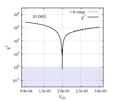
Figure 2: Variation of $\chi^{2}$ as a function of $\lambda^{\prime}_{222}$ for scenarios S2 NH, S3 IH and S3 DEG. The glitches in S3 IH and S3 DEG are associated with the ‘crossing–over’ of mass eigenstates when $\lambda^{\prime}_{222}$ is varied. See text for more discussion.

In Fig. 2, we display the changes in $\chi^{2}$ for a few selected scenarios (S2 NH, S3 IH and S3 DEG) when a LNV coupling is varied within [0.5:1.5] times the best–fit value. We define a “width” for a $\chi^{2}$ minimum to be

$$w\,\equiv\,\frac{\Delta\Lambda|_{\chi^{2}<3}}{\Lambda|_{\chi^{2}\approx 0}}\;,$$ (79)

so that a large (small) $w$ value may be interpreted as less (more) fine–tuning between different LNV couplings.

Clearly the NH case looks significantly better than the IH/DEG cases:

$$w(\mathrm{NH},\Lambda=\lambda^{\prime}_{222}) = 1.1\cdot 10^{-1}\;,$$

$$w(\mathrm{IH},\Lambda=\lambda^{\prime}_{222}) = 7.4\cdot 10^{-3}\;,$$

$$w(\mathrm{DEG},\Lambda=\lambda^{\prime}_{222}) = 4.8\cdot 10^{-4}\;.$$ (80)

In fact, since the neutrino masses in our model are free parameters to be fitted to the data, it is natural for these masses to be non–degenerate. To obtain the two (three) quasi–degenerate masses in the IH (DEG) spectrum thus requires a certain amount of fine–tuning, which should be reflected in the value of $w$. Recall from Eqs. (58) and (59) that due to a small (zero) $\sin[\theta_{13}]$ in the near (exact) TBM limit, there are small off–diagonal entries for an inverted or degenerate mass spectrum. Specifically, $\alpha_{21}$ is small in both cases, while $\alpha_{31}$ is also small in a DEG spectrum. As a result, there are small off–diagonal entries for both IH and DEG scenarios but not for a normal hierarchy, while in our set–up the diagonal and off–diagonal entries of $M_{\alpha}$ are of the same order for each $\alpha$. Therefore, a way to understand this fine tuning technically would be by considering the size of the off–diagonal entries of $\mathcal{M}_{\nu}^{{\rm eff}}$. We discuss the three cases separately.

In the case of NH, the off–diagonal entries in $\mathcal{M}_{\nu}^{{\rm eff}}$ will be of the same order as the diagonal values. In this case, the experimental observables are fairly insensitive to changes of up to $\mathcal{O}(10\%)$ in the LNV sector, cf. Eq. (80).

For IH, we have two nearly degenerate mass eigenstates. Therefore, the tree–level and the loop contribution have to be of the same order, with a near–cancellation occurring between the off–diagonal entries of $M_{1}$ and $M_{2}$. This results in a significantly larger width of the $\chi^{2}$ minimum than in the NH case.

For the same reason, in the DEG cases even larger fine–tuning is required in order to obtain three nearly degenerate neutrino masses. Actually, in the limit $M\gg\Delta M\sim\Delta m^{2}/M$, where $M$ is the mass scale of the heaviest neutrino, all off–diagonal entries will have a magnitude of $\mathcal{O}(\Delta M)$, and the width $w$ can be approximated by

$$\Lambda^{2} \sim M\,,$$ (81)

$$\frac{\Delta\Lambda}{\Lambda} \sim \frac{1}{2}\frac{\Delta M}{M}.$$ (82)

A consequence of such fine–tuning is that if $\mathcal{M}_{\nu}^{{\rm eff}}$ is deformed slightly (for example due to changes in model parameters or technical aspects such as low convergence threshold in the spectrum calculation), the angles can change a lot since they are especially sensitive to the (small) off–diagonal entries of $\mathcal{M}_{\nu}^{{\rm eff}}$. In contrast, the mass values are much more stable, with their sum determined by the diagonal entries of $\mathcal{M}_{\nu}^{{\rm eff}}$.

This can be illustrated by changing the implementation of the LNV parameters in the numerical code from 6 significant figures to 3: the masses change by less than 1 percent, whereas the angles change by a factor of order one. Therefore the values displayed in Table 3, especially those for the IH and DEG cases, need to be taken with caution. However, listing more digits would result in worse readability, so we ask readers interested in reproducing our results to contact the authors for more precise values.

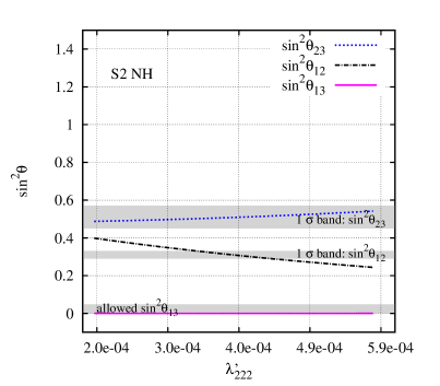
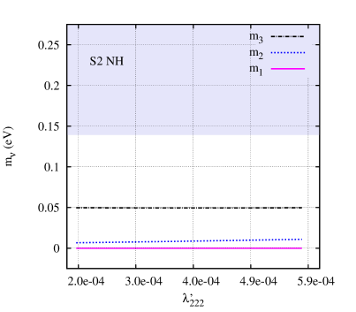
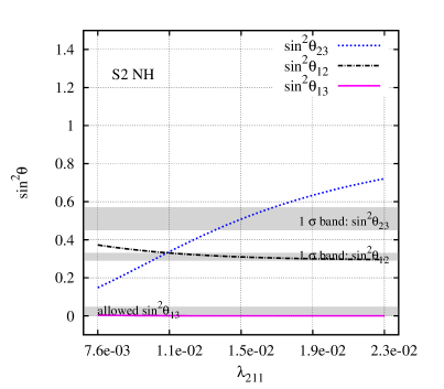
Figure 3: Variation of the mixing angles (left) and the mass eigenvalues (right) as functions of $\lambda^{\prime}_{222}$ (top) and $\lambda_{211}$ (bottom) for scenario S2 NH. The best fit values for $\lambda^{\prime}_{222}$ and $\lambda_{211}$ are located at the centre of the plots. On the plots of mixing angles, the grey bands are experimentally viable regions for (from top to bottom) ${\rm sin}^{2}\theta_{23}$, ${\rm sin}^{2}\theta_{12}$ and ${\rm sin}^{2}\theta_{13}$. On the plots of mass eigenvalues, values inside the grey bands are disfavoured by cosmological considerations.

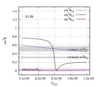
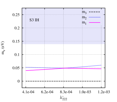
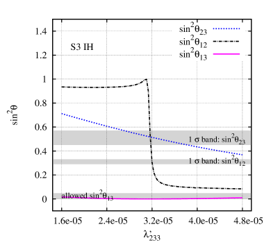
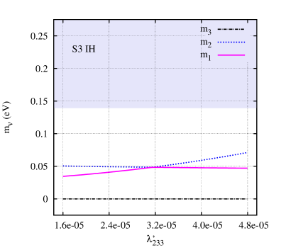
Figure 4: Variation of the mixing angles (left) and the mass eigenvalues (right) as functions of $\lambda^{\prime}_{222}$ (top) and $\lambda^{\prime}_{233}$ (bottom) for scenario S3 IH. The best–fit values of $\lambda^{\prime}_{222}$ and $\lambda^{\prime}_{233}$ are located at the centre of the plots. On the plots of mixing angles, the grey bands are experimentally viable regions for (from top to bottom) ${\rm sin}^{2}\theta_{23}$, ${\rm sin}^{2}\theta_{12}$ and ${\rm sin}^{2}\theta_{13}$. On the plots of mass eigenvalues, values inside the grey bands are disfavoured by cosmological considerations.

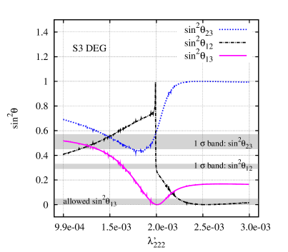
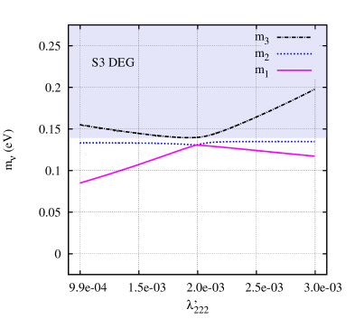
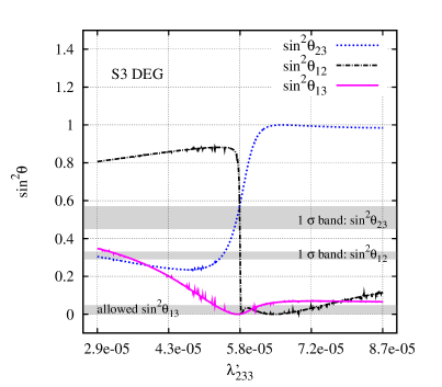
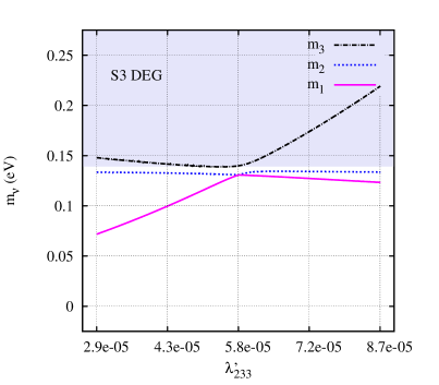
Figure 5: Variation of the mixing angles (left) and the mass eigenvalues (right) as functions of $\lambda^{\prime}_{222}$ (top) and $\lambda^{\prime}_{233}$ (bottom) for scenario S3 DEG. The best fit values for $\lambda^{\prime}_{222}$ and $\lambda^{\prime}_{233}$ are located at the centre of the plots. On the plots of mixing angles, the grey bands are experimentally viable regions for (from top to bottom) ${\rm sin}^{2}\theta_{23}$, ${\rm sin}^{2}\theta_{12}$ and ${\rm sin}^{2}\theta_{13}$. On the plots of mass eigenvalues, values inside the grey bands are disfavoured by cosmological considerations.

To see how the experimental observables change as the LNV couplings are varied, we show in Figs. 3, 4 and 5 the variation of the mixing angles and masses as functions of $\lambda^{\prime}_{222}$. Recall that the $\chi^{2}$ variation of the fit for $\lambda^{\prime}_{222}$ is displayed in Fig. 2. For illustrative purposes these figures also show the variation of another LNV coupling for each of these scenarios, such that two sets of couplings, each corresponding to one $M_{\alpha}$, are presented ref:footnote13 .

We first discuss the scenario S2 NH, which is illustrated in Fig. 3. In the upper two plots, one sees that the variation of $\lambda^{\prime}_{222}$ mainly affects $\theta_{12}$ and somewhat also $m_{2}$, whereas $\theta_{23}$ and $m_{3}$ are left relatively unchanged. In the lower two plots, where $\lambda_{211}$ is varied, the observables are reversely affected. This is because the two non–zero mass matrices, $M_{2}\sim m_{\nu 2}$ and $M_{3}\sim m_{\nu 3}$, are controlled by the $\lambda$ and $\lambda^{\prime}$ couplings separately (i.e. by the tree–level and loop level contribution, respectively). Obviously, in NH $\sin^{2}\theta_{12}$ is determined only by $M_{2}$, whereas in IH and DEG, the form of $M_{1}$ is also relevant. Therefore, NH is the easiest scenario to fit, because the observables can be directly related to independent sets of couplings. The mixing ${\rm sin}^{2}\theta_{13}$ remains practically unchanged due to our ansätz in Eq. (75), which is designed to give a tiny $\theta_{13}$.

For scenario S3 IH (Fig. 4), we see that here, no clean correlation exists between which LNV parameter is varied and which observable is affected. $\theta_{12}$ and $m_{2}$ change drastically and are affected by both $\lambda^{\prime}_{i22}\sim M_{1}$ and $\lambda^{\prime}_{i33}\sim M_{2}$. The sharp change in ${\rm sin}^{2}\theta_{12}$ around the best–fit point corresponds to “cross–overs” of mass eigenstates $m_{1}$ and $m_{2}$ as $\lambda^{\prime}_{222}$ or $\lambda^{\prime}_{233}$ is varied. The fact that the best–fit solution lies in this steeply changing region simply reflects the fact that for IH the two heavy neutrinos have similar masses. Incidentally, the small “suppression” at $\lambda^{\prime}_{222}\sim-8.4\cdot 10^{-4}$ in the corresponding $\chi^{2}$ plot in Fig. 2 near the best–fit point corresponds to a region where $\Delta m^{2}_{21}$ coincides with the experimental value during this cross–over. However to a reasonable approximation the flavour content of the two mass eigenstates are now swapped, hence ${\rm sin}^{2}\theta_{12}$ is different from its best–fit value.

On the other hand, it is clear that $m_{3}$ does not sit close to the cross–over region. Moreover, since $m_{3}$ basically contains only $\mu$ and $\tau$ flavours around the best–fit region, the proportion of $\mu$ and $\tau$ content of the other two mass eigenstates must be the same in order for them to be orthogonal to $m_{3}$. As a consequence, the cross–over of these two states only changes $\sin^{2}\theta_{23}$ mildly. As in the case of S2 NH, $\sin^{2}\theta_{13}$ is designed to have a tiny value.

For the scenario S3 DEG (Fig. 5), the fact that the three mass scales are very close to each other means that complete separation of the three contributions is in practice very difficult. As in S3 IH, the best–fit point lies close to a region where cross–over of mass eigenstates take place. In this case, two cross–overs take place near the best–fit point. For example, the non–trivial variation of ${\rm sin}^{2}\theta_{12}$ with $\lambda^{\prime}_{233}$ immediately to the right of the best–fit point corresponds to a second cross–over of the mass eigenvectors. The fact that all three masses are quasi–degenerate also explains the large transition of all three mixing angles. In particular, even though the coupling set is chosen to have a small ${\rm sin}^{2}\theta_{13}$, immediately away from the best–fit point the mass ordering is changed, resulting in the different ${\rm sin}^{2}\theta_{13}$ behaviour compared with the NH and IH cases.

Furthermore, due to the strong fine–tuning, the $\chi^{2}$ suppression expected as in the IH scenarios is buried within the rapidly increasing $\chi^{2}$ value. We note in passing that due to this fine–tuning, the numerical results are less stable than those in the NH and IH scenarios. This results in the fluctuations seen in the figures ref:footnote11 .

We now go on to discuss the scenarios S4, which represent scenarios with the smallest possible LNV couplings to still describe the oscillation data correctly. In the S4 NH scenario, recall that the antisymmetry of the $\lambda_{i33}$ couplings generates zeros in $M_{3}$ which do not correspond to the “texture zeros” given in Eq. (58). Therefore, linear combinations between the different contributions to the neutrino masses (i.e. between $M_{2}\sim m_{\nu 2}$ and $M_{3}\sim m_{\nu 3}$) are necessary to obtain the desired oscillation parameters. As a result, the ratio of the couplings are not approximated by those displayed in Eq. (65) but instead by a linear combination of these, cf. Ref. ref:footnote6 . Still, the behaviour of the observables when the relevant LNV couplings are varied is similar to the scenarios discussed above.

In the S4 IH scenario, the $\lambda^{\prime}_{i33}$ couplings still roughly follow the expected structure and magnitude as before in S1 to S3 IH. However, the deviations are slightly larger because of the presence of $\lambda$ couplings. In contrast to other IH scenarios, in S4 IH, $M_{2}$ is generated at tree–level from $\lambda_{i33}$ and $\lambda_{322}$ instead of at 1–loop level from $\lambda^{\prime}_{i22}$. The absence of $\lambda_{333}$, due to anti–symmetry of the first two generation indices, means that $\lambda_{322}$ (or $\lambda_{311}$) is needed to “fill up” the third row/column of the tree–level matrix $M_{2}$. In this scenario, all diagonal third generation couplings are used. Consequently, the magnitude of our coupling set is the smallest possible among the diagonal inverted hierarchy scenarios.

The ratio of the three $\lambda$ couplings is approximately

$$(\lambda_{133}:\lambda_{233}:\lambda_{322})\;\sim\;(1\,:\,1\,:\,-16)\,,$$ (83)

which is expected as these couplings scales as $1/(Y_{E})_{ii}$ ($i=2,3$).

We conclude in both the NH and the IH case that it is not possible to push all LNV couplings below $\mathcal{O}(10^{-5})$. However, at this order of magnitude, displaced vertices might be observed at colliders, depending on the benchmark point, cf. Sect. VI.

V.2 Off–diagonal LNV Scenarios

In S5 we present the solutions for the two off–diagonal LNV scenarios. We see that the NH off–diagonal solution, being an example of non–hierarchical off–diagonal couplings, is very similar to the diagonal NH solutions in structure, cf. Eq. (83). Obviously, because here the generation indices of the couplings are $i23/i32$ instead of $i22$ (S2) or $i33$ (S3). The order of magnitude of the couplings is somewhere between the solutions S2 and S3, mirroring the mass hierarchy in the down–quark sector.

In scenario S5 DEG, the $\lambda_{231}$ coupling is much larger than the other couplings, representing an example of a strongly hierarchical off–diagonal scenario. In fact,when performing the SOFTSUSY  pre–iteration for our benchmark point, we found $\lambda_{231}$ to be of $\mathcal{O}(1)$, which is inconsistent with the requirement of perturbativity, and also violates the low–energy bounds.

To reduce the size of this coupling, a different cSSM benchmark point is therefore chosen. Employing a larger ${\rm tan}\beta$ and also ${\rm sgn}(\mu)=-1$ is useful, as the former implies larger down–type quark Yukawa couplings, while the latter also increases certain loop contributions to neutrino masses. Of course, assuming a heavier mass spectrum is also helpful. In fact, a scan over the cSSM parameter space with the condition $\lambda_{231}\lesssim\mathcal{O}(0.1)$, leads to the following benchmark point (BP2):

$$M_{1/2} = 760\textrm{ GeV}\,,$$

$$M_{0} = 430\textrm{ GeV}\,,$$

$${\rm tan}\beta = 40\,,$$

$${\rm sgn}(\mu) = -1\,.$$ (84)

The $A_{0}^{(\lambda^{\prime})}$ corresponding to this is 1059.2 GeV. The resulting mass spectrum is displayed in Table 5. Compare with the original benchmark point BP, the sparticles in BP2 are somewhat heavier than those in BP. Also, while the LSP in BP is a stau, the relatively small differences between $M_{1/2}$ and $M_{0}$ in BP2 results in a neutralino LSP ($\tilde{\chi}^{0}_{1}$) instead. This leads to distinctly different collider phenomenology, which will be briefly discussed in the next section.

Particles	Masses (GeV)
$\tilde{g}$	1696
$\tilde{\chi}^{\pm}_{1},\tilde{\chi}^{\pm}_{2}$	599	798
$\tilde{\chi}^{0}_{1},\tilde{\chi}^{0}_{2},\tilde{\chi}^{0}_{3},\tilde{\chi}^{0}_{4}$	320	599	785	799
$\tilde{u}_{1},\tilde{c}_{1},\tilde{t}_{1}$	1593	1593	1431
$\tilde{u}_{2},\tilde{c}_{2},\tilde{t}_{2}$	1536	1535	1281
$\tilde{d}_{1},\tilde{s}_{1},\tilde{b}_{1}$	1595	1595	1427
$\tilde{d}_{2},\tilde{s}_{2},\tilde{b}_{2}$	1530	1530	1358
$\tilde{e}_{1},\tilde{\mu}_{1},\tilde{\tau}_{1}$	665	665(663)	631(629)
$\tilde{e}_{2},\tilde{\mu}_{2},\tilde{\tau}_{2}$	516(510)	515	382
$\tilde{\nu}_{e},\tilde{\nu}_{\mu},\tilde{\nu}_{\tau}$	659	659(657)	616(614)
$h^{0},A^{0},H^{0},H^{\pm}$	116	579	577	585

Table 5: Mass spectrum of the benchmark point BP2 in the $R_{p}$ conserving limit. The notation is the same as Table 1. The values in brackets denote changes when the non–zero LNV couplings in S5 DEG is included. As expected, the dominant coupling $\lambda_{231}$ changes the second and third generation slepton and the (right–handed) selectron masses, but only by at most 1%.

V.3 Effects of changing the benchmark point

So far, we have only considered scenarios under the assumption of up–mixing in the quark sector and using the $A_{0}^{(\lambda^{\prime})}$ minimum. In the rest of this section we briefly discuss changes which occur when down–mixing is assumed or using the $A_{0}^{(\lambda)}$ minimum instead.

• $A_{0}^{(\lambda)}$ minimum: We consider as an example the scenario S2 NH. The best–fit LNV couplings for $A_{0}^{(\lambda^{\prime})}=912.3$ GeV are given in the second row, first column of Table  3. When using the $A_{0}^{(\lambda)}$ minimum instead (given by $A_{0}^{(\lambda)}=200.6$ GeV), the $\lambda^{\prime}_{i22}$ couplings generate $M_{2}$ at tree–level whereas $M_{3}$ is generated by $\lambda_{i11}$ at one–loop level (for the $A_{0}^{(\lambda^{\prime})}$ it was the other way round). We obtain as a best fit

  $$\lambda^{\prime}_{122} = \>\>\>\,1.11\cdot 10^{-5}$$

  $$\lambda^{\prime}_{222} = \>\>\>\,1.49\cdot 10^{-5}$$

  $$\lambda^{\prime}_{322} = -8.99\cdot 10^{-6}$$

  $$\lambda_{211} = \>\>\>\,{\bf\mathbf{1.53\cdot 10^{-1}}\>[b3],[b5]}$$

  $$\lambda_{311} = \>\>\>\,{\bf\mathbf{1.59\cdot 10^{-1}}\>[b4]}$$ (85)

  The decrease (increase) by a factor 10 of the $\lambda^{\prime}_{i22}$ ($\lambda_{i11}$) couplings reflects the typical hierarchy between the tree–level and the one–loop neutrino mass of $\mathcal{O}(10^{2})$, cf. Fig. 1. In contrast to the original S2 NH scenario, this scenario is not compatible with several low–energy bounds as listed in Sect. II.6 due to the larger $\lambda_{i11}$ couplings.

• down–mixing: When changing the quark mixing assumption from up–type to down–type mixing, cf. Sec. II.4, the LNV parameters are affected via RG running. However, the changes when running from the unification scale down to the electroweak scale are less than 1 percent for diagonal LNV couplings when switching from up–type to down–type mixing. This is because for $\lambda^{\prime}$ couplings involving light generations (e.g. $\lambda^{\prime}_{i11}$), RG running is dominated by gauge contributions. For couplings involving the third generation (e.g. $\lambda^{\prime}_{i33}$), the fact that the only significant mixing in the CKM matrix is between the first two generations implies that the effect of changing the quark mixing is also small. The bilinear LNV couplings responsible for the tree level neutrino mass matrix are dynamically generated by $\lambda$ couplings, which are of course not affected directly by changes in the quark mixing assumptions. In models where bilinear couplings are generated by $\lambda^{\prime}$ couplings, the effect of changing the quark mixing assumption is more complicated.

  Note also that for non–diagonal couplings, the changes are expected to be much larger than for diagonal couplings. This is because $Y_{D}$ is diagonal when assuming up–quark mixing, while non–zero off–diagonal entries are present when down–quark mixing is assumed instead. We note that similar observations are made in Ref. Dreiner:2010ye , where a single non–zero LNV coupling is used to saturate the cosmological bound.

  Nevertheless, these small changes for diagonal LNV couplings can still be important, particularly for the IH and DEG scenarios, which are sensitive to the exact values of the LNV parameters. On top of that, 1–loop contributions involving light quark mass insertions can depend sensitively on the quark mixing assumption. For example, $(Y_{D})_{11}$ changes by a factor of $\sim 2$ when the mixing is changed, which implies large changes in the loop contributions involving $\lambda^{\prime}_{i11}$, which in turn will affect all mass ordering scenarios. In contrast, $(Y_{D})_{22}$ changes by a couple of percent, so the impact through the mass insertion is relatively mild.

  In principle, changing the mixing assumption, but retaining the same coupling values, can affect $\chi^{2}$ dramatically, if the width $w$ of the scenario is small. As a numerical example consider a comparison of the three scenarios depicted in Fig. 2. S2 NH, involves $\lambda^{\prime}_{i22}$ with a width $w$ of $\mathcal{O}(10\%)$. Here $\chi^{2}$ increases from $\sim 0$ in the up–mixing case to about $3$ in the down–mixing case. In contrast, in S3 IH (DEG), where the width is narrower than $1\%$ ($0.1\%$), changing the quark mixing assumption leads to a $\chi^{2}$ change of 4 (more than 6) orders of magnitude. These changes can be compensated by refitting the LNV couplings. It is not surprising that refitting a subset of couplings is sufficient. For example, a refit of S3 IH yields:

  $$\lambda^{\prime}_{122} = \>\>\>\,1.70\cdot 10^{-3}$$

  $$\lambda^{\prime}_{222} = -8.80\cdot 10^{-4}$$

  $$\lambda^{\prime}_{322} = \>\>\>\,9.71\cdot 10^{-4}$$

  $$\lambda^{\prime}_{133} = \>\>\>\,3.11\cdot 10^{-5}$$

  $$\lambda^{\prime}_{233} = \>\>\>\,3.22\cdot 10^{-5}$$

  $$\lambda^{\prime}_{333} = -3.32\cdot 10^{-5}\,,$$ (86)

  where the three $\lambda^{\prime}_{i22}$ are refitted. A different solution with a small $\chi^{2}$ can also be obtained by refitting $\lambda^{\prime}_{i33}$ alone. The solution in Eq. (• ‣ V.3) differs from the original up–type mixing solution by $\mathcal{O}(10\%)$. This is what one might expect, bearing in mind that the changes occurring in the CKM matrix from up–type to down–type mixing are $\sim 20\%$.

VI Collider signatures

The neutrino models we have found in the previous sections lead to observable collider signatures. Here, we shortly discuss phenomenological implications at the LHC. Resonant slepton production typically requires a coupling strength $\lambda^{\prime}_{i11}\stackrel{{\scriptstyle>}}{{\sim}}10^{-3}$ for incoming first generation quarks Dreiner:2000vf . For higher generation quarks an even larger coupling is required to compensate the reduced parton luminosity. In Table 3, we see that our models do not satisfy this requirement. However, by considering a scenario which combines aspects of S1 NH and S4 NH, it is possible to have a large $\lambda^{\prime}_{211}$ while evading the low energy constraints, see ref:footnote18 .

Thus in most neutrino mass scenarios, squark and gluino production are the dominant production mechanisms for supersymmetric particles at the LHC, as in the $R_{p}$ conserving MSSM. Once produced, the squarks and gluinos cascade decay in the detector to the LSP, via gauge couplings. The final LHC signature is then determined by the exact nature of the LSP and the LNV operators leading to the LSP decay.

For our benchmark point BP, we have a stau LSP $\tilde{\tau}_{2}$ ref:footnote17 and the NLSP is the lightest neutralino $\tilde{\chi}_{1}^{0}$ with $m_{\tilde{\tau}_{2}}=163$ GeV and $m_{\tilde{\chi}_{1}^{0}}=204$ GeV. A typical production process for our BP parameters is then given by

$$pp\rightarrow\tilde{q}\tilde{q}\rightarrow qq\tilde{\chi}_{1}^{0}\tilde{\chi}_{1}^{0}\rightarrow qq\tau\tau\tilde{\tau}_{2}\tilde{\tau}_{2}.$$ (87)

Here we have employed BR($\tilde{\chi}_{1}^{0}\rightarrow\tilde{\tau}_{2}\tau)=1$, which is by far the dominant decay mode in our BP. The LSP stau can normally decay via two– and four–body modes Dreiner:2008rv . However, in our $B_{3}$ cSSM neutrino models we always have a non–zero LNV operator which directly couples to the stau LSP. Thus the stau will dominantly decay into two SM fermions and the four–body decays of the stau LSP are highly suppressed. The collider signatures can then be classified by the possible two–body stau decay modes, as well as the stau decay length. A recent detailed discussion of stau LSP phenomenology at the LHC is given in Ref. Desch:2010gi . However, this focuses on four–body stau decay modes.

For S2 NH, S3 NH, S5 NH and S3 DEG, we find that $\lambda_{311}$ is the dominant LNV operator which is relevant for the tree–level two–body stau decay. Assuming the cascade decay in Eq. (87) we expect as the final state collider signature

$$2j+2\ell+2\tau+2\nu.$$ (88)

In this case $\ell=e$. Note that the final state charged leptons can have the same electric charge, since the intermediate NLSP neutralinos in Eq (87) are Majorana fermions. Like–sign dilepton signatures at the LHC in the context of ${{\not\!{R}}_{p}}$ have been studied extensively in the literature, see for example Dreiner:1993ba ; likesign ; Dreiner:2000vf . Here we could in addition also make extra use of the final state tau leptons, as in Ref. Desch:2010gi .

In S4 NH and S4 IH the stau LSP cannot decay via $\lambda^{\prime}_{333}$, because it is kinematically forbidden, as $m_{\tilde{\tau}_{2}}<m_{\rm top}$. Instead it will decay via $\lambda_{133},\,\lambda_{233}$, or $\lambda_{322}$ to a two–body leptonic final state. Hence, in both scenarios the stau LSP decays into two leptons and we expect the same signature as in Eq. (88). However, the couplings have typical values of the order of $10^{-6}$–$10^{-5}$. The stau lifetime is given by

$$\tau_{\tilde{\tau}} = \left[\Gamma(\tilde{\tau}\rightarrow f_{1}+f_{2})\right]^{-1}=\frac{16\pi}{N_{c}\Lambda^{2}m_{\tilde{\tau}_{2}}}$$ (89)

$$= 3.3\cdot 10^{-15}\,\mathrm{sec}\frac{1}{N_{c}}\left(\frac{100\,\mathrm{GeV}}{m_{\tilde{\tau}_{2}}}\right)\left(\frac{10^{-5}}{\Lambda}\right)^{2}\!\!.$$

Here $N_{c}$ is the colour factor. It is $3$ for $\lambda^{\prime}$ couplings and $1$ for $\lambda$ couplings. We have ignored any factors due to stau mixing and have only considered one dominant decay mode ref:footnote16 . The decay length is then given by

$$L_{\tilde{\tau}_{2}} = \gamma\beta c\tau_{\tilde{\tau}_{2}}$$ (90)

$$= \gamma\beta\cdot 10^{-6}m\cdot\frac{1}{N_{c}}\left(\frac{100\,\mathrm{GeV}}{m_{\tilde{\tau}_{2}}}\right)\left(\frac{10^{-5}}{\Lambda}\right)^{2}.$$

In S4 NH the stau mass is 163 GeV and $c\tau_{\tilde{\tau}_{2}}\sim 3\mu$m. The benchmark point BP implies that at the 14TeV LHC $\gamma\beta$ is typically of $\mathcal{O}({\rm few})$. Therefore a small fraction of events, with $\gamma\beta$ for one of the stau LSPs near 10, could lead to detached vertices that are observable at the LHC displaced .

S3 IH is special. Here we just allow for non–zero $\lambda^{\prime}_{ijk}$ couplings. Hence, the stau LSP has only one hadronic two–body decay mode via $\lambda^{\prime}_{322}$, $\tilde{\tau}_{2}\rightarrow c+s$. The final state collider signature is

$$6j+2\tau.$$ (91)

This is very difficult to observe. One must then consider other cascades with intermediate first or second generation sleptons. These lead to additional leptons in the final state. However, the corresponding overall branching ratios are smaller.

For our benchmark point BP2, we have a neutralino LSP with $m_{\tilde{\chi}_{1}^{0}}=320$ GeV. A typical production process for BP2 is given by

$$pp\rightarrow\tilde{q}\tilde{q}\rightarrow qq\tilde{\chi}_{1}^{0}\tilde{\chi}_{1}^{0}.$$ (92)

For S5 DEG, the dominant LNV coupling is $\lambda_{231}$ and the neutralino LSP decays via an off–shell slepton as

$$\tilde{\chi}_{1}^{0}\rightarrow\mu^{\pm}e^{\mp}\nu_{\tau},\;\tau^{\pm}e^{\mp}\nu_{\mu}\,,$$ (93)

and we did not distinguish between neutrinos and anti–neutrinos here. We then expect the following event topologies

$$2j+2\nu+\left\{\begin{array}[]{l}2\ell+2\tau,\\ 3\ell+1\tau,\\ 4\ell,\end{array}\right.$$ (94)

where the branching ratios for all channels are roughly the same.

VII Summary and Outlook

Experimentally it is now well established that the neutrinos are massive and have non–vanishing mixing angles. This requires physics beyond the Standard Model. In this paper we have reanalyzed the neutrino mass and mixing data in the light of supersymmetric R–parity violating models. These automatically include lepton number violation, and thus Majorana neutrino masses. One neutrino mass is generated at tree–level via mixing with the conventional neutralinos. Any further neutrino masses must arise at the one–loop level. We have improved the accuracy of the neutrino mass and mixing angle computation, in particular we have performed a full one loop calculation for the sneutrino vacuum expectation values, on top of the one loop corrections to the neutral fermion masses. This computation is implemented as an extension to the mass spectrum calculational tool SOFTSUSY Allanach:2001kg ; Allanach:2009bv .

Most importantly, we have implemented also for the first time in the construction of neutrino mass models, a mechanism to suppress the tree–level masses compared to the corresponding 1–loop contribution. This requires a tuning, but not fine–tuning, of the tri–linear soft breaking $A_{0}$ parameter. This allows much larger flexibility in the fitting procedure. It also allows for solutions with larger lepton number violating couplings.

In this region of the $A_{0}$ parameter space, there are a large number of possibilities to obtain the observed neutrino masses and mixings. We have split our analysis into normal hierarchy (NH), inverted hierarchy (IH) and degenerate (DEG) models. Furthermore we have mostly focused on one benchmark point to fix the other cSSM parameters. We have implemented all the relevant low–energy bounds on the lepton number violating R–parity violating couplings. It turns out these kill a significant number of the best–fit solutions we find.

We have then considered five different scenarios, labelled S1 through S5. Scenarios S1 through S3 employ diagonal lepton number violating couplings $\Lambda_{ijk},\;j=k$ and the couplings are chosen to closely follow the structure of the tri–bi maximal mixing solutions. The three scenarios correspond to the three different possible generations $j=k=1,2,3$. Higher generations lead to smaller lepton number violating couplings, because the corresponding Higgs Yukawa couplings which also enter the formulae are larger.

In looking for solutions, we then fit a small number of lepton number violating couplings to the neutrino data. We need five couplings in the NH case, six in the IH case and eight couplings for the degenerate case. Our results are presented in Table 3.

Solutions with large couplings, $\Lambda=\mathcal{O}(10^{-2})$, are mostly excluded by the low–energy bounds. In particular this kills all S1 models, as well as the IH and DEG models in the S2 scenarios. The NH S2, as well as the NH and DEG S3 scenarios include $LL\bar{E}$ couplings of order $10^{-2}$. All other remaining scenarios have couplings $10^{-3}$ or smaller.

Possible alternatives to the scenarios S1, S2 and S3 are presented in scenarios S4 and S5. The S4 models assume ansätze with diagonal $\Lambda$ couplings but alternative methods to obtain the neutrino masses, whereas the S5 models employ off–diagonal $\Lambda$ couplings. We have not attempted to construct IH S5 nor DEG S4 models.

All models lead to observable effects at colliders, as the LSP will always decay in the detector. These have been discussed in detail elsewhere. Characteristic of all neutrino models is that we should get signatures which violate at least two lepton flavors. For the case of S4 scenarios, where all couplings are $|\Lambda|<5\cdot 10^{-5}$ there could possibly be detached vertices.

In performing the numerical fit, we use a multistep procedure. We start with initial values estimated from upper bounds on the neutrino mass from WMAP. Then we perform separate pre–iterations for the tree– as well as for the 1–loop contributions in SOFTSUSY. This already gives a good estimate. The final solution is then found by minimizing the $\chi^{2}$ function with the program package MINUIT2, where all tree– and 1–loop level contributions simultaneously contribute to the neutrino mass matrix. The degenerate scenarios require some fine–tuning, thus we have implemented a Markov chain Monte Carlo method to obtain the experimentally observed neutrino data.

We find that all three neutrino mass hierarchies are possible, which can contribute to $0\nu\beta\beta$ through the standard light neutrino exchange. However these simple models suggest normal hierarchy (NH) might be preferred, so that the mass contribution to $0\nu\beta\beta$ will not be probed by the next generation of $0\nu\beta\beta$ experiments. All our models involving $\lambda^{\prime}_{111}$ couplings strongly violate the limit from its contribution to $0\nu\beta\beta$ through the so–called direct neutralino/gluino exchange mechanism. In other words, if $0\nu\beta\beta$ is dominated by the direct exchange mechanism, $\lambda^{\prime}_{111}$ is unlikely to contribute significantly to the neutrino masses.

Despite the tension between the neutrino mass contribution and the low energy bounds, which favor large and small LNV couplings respectively, $\lambda$ couplings of $\mathcal{O}(0.01)$ (e.g. S2, S3 NH) involving only the first 2 lepton generations are allowed. However, simultaneous presence of (dominant) diagonal LNV couplings $\lambda^{\prime}_{i11}$ and $\lambda_{j11}$ appears to be difficult, at least with the assumed mass spectrum BP. Single coupling dominance, which many collider studies usually assume, also appears to be consistent with neutrino oscillation data (S5 DEG). It would therefore be interesting to study collider implications of these models in more detail in the future.