A momentum-space Argonne V18 interaction

Abstract

This paper gives a momentum-space representation of the Argonne V18 potential as an expansion in products of spin-isospin operators with scalar coefficient functions of the momentum transfer. Two representations of the scalar coefficient functions for the strong part of the interaction are given. One is as an expansion in an orthonormal basis of rational functions and the other as an expansion in Chebyshev polynomials on different intervals. Both provide practical and efficient representations for computing the momentum-space potential that do not require integration or interpolation. Programs based on both expansions are available as supplementary material. Analytic expressions are given for the scalar coefficient functions of the Fourier transform of the electromagnetic part of the Argonne V18. A simple method for computing the partial-wave projections of these interactions from the operator expressions is also given.

I Introduction

The Argonne V18 potential v18 is one of a number of nucleon-nucleon interactions reid v18 cdbonn that provide a quantitative description of experimental two-body observables below the pion-production threshold. It is distinguished from the other realistic interactions because it is expressed as an operator expansion with local configuration-space coefficient functions. This representation has advantages when used in variational Monte Carlo calculations. On the other hand, there are a number of calculations that require a realistic interaction that are more naturally performed in momentum space. These include some Faddeev calculations, relativistic few-body calculations, and calculations involving electromagnetic probes. In the momentum representation the variable conjugate to the relative coordinate is the momentum transfer. In calculations, both momenta appear, which requires either an interpolation or a separate Fourier transform for each pair of momenta. Fourier transforms of the V18 potential have been used in some applications huber . The purpose of this paper is to provide useful, tested and reproducible analytic approximations of the Fourier transform of the Argonne V18 potential for use in momentum-space calculations. The analytic forms allow for a direct calculation of the momentum-space interaction for any pair of initial and final momenta. In keeping with the traditional Argonne form, the momentum-space potential is given as a linear combination of products of spin-isospin operators with scalar functions of the momentum transfer. The resulting momentum-space potential has 24 terms. The additional six operators appear because the Fourier transform of the terms involving the operators $\mathbf{L}^{2}V_{i}(r)$ and $(\mathbf{L}\cdot\mathbf{S})^{2}V_{i}(r)$ each become a sum of two different momentum-space operators with different coefficient functions. In this work the Fourier transform is given for the strong part of the Argonne V18 potential, without the electromagnetic terms. This part of the potential must be treated numerically. The electromagnetic terms have analytic Fourier transforms, which are discussed in Appendix   3. The partial-wave projection of the momentum space potential is discussed in Appendix   2. It is constructed from the operator expressions by integrating over the angle between the initial and final momentum vectors, however unlike the configuration-space partial-wave projection, the integrals involve both the operator and the scalar coefficient functions.

The Argonne V18 potential has the form

$$V=\sum_{n=1}^{18}V_{n}(r)O_{n}$$ (1)

where $V_{n}(r)$ are rotationally-invariant coefficient functions of the relative coordinate of the nucleons and the $O_{n}$ are the eighteen spin-isospin operators given in Table 1.,

Table 1: Argonne V18 spin-isospin operators

in coordinate-space Term spin-isospin Operator in r-space $O_{1}$ $\mathbf{I}$ $O_{2}$ $(\mbox{\boldmath$\tau$}_{1}\cdot\mbox{\boldmath$\tau$}_{2})$ $O_{3}$ $(\boldsymbol{\sigma}_{1}\cdot\boldsymbol{\sigma}_{2}),$ $O_{4}$ $(\boldsymbol{\sigma}_{1}\cdot\boldsymbol{\sigma}_{2})(\mbox{\boldmath$\tau$}_{1}\cdot\mbox{\boldmath$\tau$}_{2})$ $O_{5}$ $S_{12}=3(\boldsymbol{\sigma}_{1}\cdot\hat{\mathbf{r}})(\boldsymbol{\sigma}_{2}\cdot\hat{\mathbf{r}})-\boldsymbol{\sigma}_{1}\cdot\boldsymbol{\sigma}_{2}$ $O_{6}$ $S_{12}(\mbox{\boldmath$\tau$}_{1}\cdot\mbox{\boldmath$\tau$}_{2}),$ $O_{7}$ $(\mathbf{L}\cdot\mathbf{S})$ $O_{8}$ $(\mathbf{L}\cdot\mathbf{S})(\mbox{\boldmath$\tau$}_{1}\cdot\mbox{\boldmath$\tau$}_{2})$ $O_{9}$ $(\mathbf{L}\cdot\mathbf{L})$ $O_{10}$ $(\mathbf{L}\cdot\mathbf{L})(\mbox{\boldmath$\tau$}_{1}\cdot\mbox{\boldmath$\tau$}_{2})$ $O_{11}$ $(\mathbf{L}\cdot\mathbf{L})(\boldsymbol{\sigma}_{1}\cdot\boldsymbol{\sigma}_{2})$ $O_{12}$ $(\mathbf{L}\cdot\mathbf{L})(\boldsymbol{\sigma}_{1}\cdot\boldsymbol{\sigma}_{2})(\mbox{\boldmath$\tau$}_{1}\cdot\mbox{\boldmath$\tau$}_{2})$ $O_{13}$ $(\mathbf{L}\cdot\mathbf{S})^{2}$ $O_{14}$ $(\mathbf{L}\cdot\mathbf{S})^{2}(\mbox{\boldmath$\tau$}_{1}\cdot\mbox{\boldmath$\tau$}_{2})$ $O_{15}$ $T_{12}=(3\tau_{1z}\tau_{2z}-\mbox{\boldmath$\tau$}\cdot\mbox{\boldmath$\tau$})$ $O_{16}$ $(\boldsymbol{\sigma}_{1}\cdot\boldsymbol{\sigma}_{2})T_{12}$ $O_{17}$ $S_{12}T_{12}$ $O_{18}$ $(\tau_{1z}+\tau_{2z})$

In this table $T_{12}$ is the isotensor operator $T_{12}:=3\tau_{1z}\tau_{2z}-\boldsymbol{\tau}_{1}\cdot\boldsymbol{\tau}_{2}$. While the isospin operators, $\boldsymbol{\tau}_{i}$, factor out of the Fourier transforms, the operators $L^{2}$, $\mathbf{L}\cdot\mathbf{S}$, $(\mathbf{L}\cdot\mathbf{S})^{2}$ and the tensor operator $S_{12}$ contribute to the Fourier transform.

The Fourier transform of this potential can be expressed as a linear combination of 24 momentum-space operators with scalar coefficient functions of the momentum transfer. There are 24 operators because the $\mathbf{L}\cdot\mathbf{L}$ and $(\mathbf{L}\cdot\mathbf{S})^{2}$ operators have two distinct contributions in momentum space. In appendix 1 it is shown that the potential matrix element $\langle\mathbf{k}^{\prime}|V|\mathbf{k}\rangle$, with $\mathbf{q}:=\mathbf{k}^{\prime}-\mathbf{k}$, has the following five types of contributions:

• $\mathbf{I}$

  $${1\over(2\pi)^{3}}\int e^{-i(\mathbf{k}^{\prime}-\mathbf{k})\cdot\mathbf{r}}V_{j}(r)\mathbf{I}d\mathbf{r}=\mathbf{I}{1\over 2\pi^{2}}\int_{0}^{\infty}j_{0}(qr)V_{j}(r)r^{2}dr.$$ (2)

• $\mathbf{L}\cdot\mathbf{S}$

  $${1\over(2\pi)^{3}}\int e^{-i\mathbf{k}^{\prime}\cdot\mathbf{r}}V_{j}(r)\mathbf{L}\cdot\mathbf{S}e^{i\mathbf{k}\cdot\mathbf{r}}d\mathbf{r}=i(\mathbf{k}\times\mathbf{k}^{\prime})\cdot\mathbf{S}{1\over 2\pi^{2}q}\int_{0}^{\infty}j_{1}(qr)V_{j}(r)r^{3}dr.$$ (3)

• $\mathbf{L}\cdot\mathbf{L}$

  $${1\over(2\pi)^{3}}\int e^{-i\mathbf{k}^{\prime}\cdot\mathbf{r}}V_{j}(r)\mathbf{L}\cdot\mathbf{L}e^{i\mathbf{k}\cdot\mathbf{r}}d\mathbf{r}=$$

  $$-(\mathbf{k}^{\prime}\times\mathbf{k})\cdot(\mathbf{k}^{\prime}\times\mathbf{k}){1\over 2\pi^{2}q^{2}}\int_{0}^{\infty}j_{2}(qr)V_{j}(r)r^{4}dr+2(\mathbf{k}^{\prime}\cdot\mathbf{k}){1\over 2\pi^{2}q}\int_{0}^{\infty}j_{1}(qr)V_{j}(r)r^{3}dr.$$ (4)

• $(\mathbf{L}\cdot\mathbf{S})^{2}$

  $${1\over(2\pi)^{3}}\int e^{-i\mathbf{k}^{\prime}\cdot\mathbf{r}}V_{j}(r)(\mathbf{L}\cdot\mathbf{S})^{2}e^{i\mathbf{k}\cdot\mathbf{r}}d\mathbf{r}=$$

  $$-(\mathbf{S}\cdot(\mathbf{k}\times\mathbf{k}^{\prime}))^{2}{1\over 2\pi^{2}q^{2}}\int_{0}^{\infty}j_{2}(qr)V_{j}(r)r^{4}dr+(\mathbf{k}^{\prime}\times\mathbf{S})\cdot(\mathbf{k}\times\mathbf{S}){1\over 2\pi^{2}q}\int_{0}^{\infty}j_{1}(qr)V_{j}(r)r^{3}dr.$$ (5)

• $S_{12}=3(\hat{\mathbf{r}}\cdot\boldsymbol{\sigma}_{1})(\hat{\mathbf{r}}\cdot\boldsymbol{\sigma}_{2})-\boldsymbol{\sigma}_{1}\cdot\boldsymbol{\sigma}_{2}$

  $${1\over(2\pi)^{3}}\int e^{-i\mathbf{k}^{\prime}\cdot\mathbf{r}}V(r)\left(3(\hat{\mathbf{r}}\cdot\boldsymbol{\sigma}_{1})(\hat{\mathbf{r}}\cdot\boldsymbol{\sigma}_{2})-\boldsymbol{\sigma}_{1}\cdot\boldsymbol{\sigma}_{2}\right)e^{i\mathbf{k}\cdot\mathbf{r}}d\mathbf{r}=$$

  $$-\left(3(\mathbf{q}\cdot\boldsymbol{\sigma}_{1})(\mathbf{q}\cdot\boldsymbol{\sigma}_{2})-q^{2}\boldsymbol{\sigma}_{1}\cdot\boldsymbol{\sigma}_{2}\right){1\over 2\pi^{2}q^{2}}\int_{0}^{\infty}j_{2}(qr)V(r)r^{2}dr.$$ (6)

These expressions are used to represent the momentum-space interaction as a sum of scalar functions of $q:=|\mathbf{q}|$ multiplied by spin-isospin operators. These scalar coefficient functions of the momentum transfer that multiply the spin-isospin operators have the form of one of the integrals listed in Table 2:

Table 2: Momentum-space scalar coefficient functions

Scalar coefficient function	dim	indices
$\tilde{V}_{m}(q):={1\over 2\pi^{2}}\int_{0}^{\infty}j_{0}(qr)V_{m}(r)r^{2}dr$	MeV fm3	$m\in\{1,2,3,4,15,16,18\}$
$\tilde{V}_{m}(q):={1\over 2\pi^{2}q}\int_{0}^{\infty}j_{1}(qr)V_{m}(r)r^{3}dr$	MeV fm5	$m\in\{7,8,9b,10b,11b,12b,13b,14b\}$
$\tilde{V}_{m}(q):={1\over 2\pi^{2}q^{2}}\int_{0}^{\infty}j_{2}(qr)V_{m}(r)r^{4}dr$	MeV fm7	$m\in\{9a,10a,11a,12a,13a,14a\}$
$\tilde{V}_{m}(q):={1\over 2\pi^{2}q^{2}}\int_{0}^{\infty}j_{2}(qr)V_{m}(r)r^{2}dr$	MeV fm5	$m\in\{5,6,17\}$

where $V_{m}(r)$ is the $m^{th}$ potential in the expansion (1) and $\tilde{V}_{ma}(q)$ and $\tilde{V}_{mb}(q)$ are the two different functions that appear in (4) and (5). These functions have finite limits as $q\to 0$ in spite of the $1/q^{l}$ coefficients since the Bessel function $j_{l}(qr)$ vanishes like $q^{l}$ as $q\to 0$. The strong interaction contribution to the 24 scalar coefficients listed in Table 2 are numerically computed. The computational methods are discussed in section 3. Programs that compute these scalar coefficients are available as supplementary material to the electronic version of this paper. Quantities, like the binding energies in the test calculations, exhibit small sensitivities (in the sixth significant figure) to the precision of input constants. In the supplementary programs these constants are taken from the original V18 potential.

The electromagnetic contribution to each of these operators can be represented in terms of known special functions. These contributions are important for precise low-energy calculations and can be added to the strong interaction coefficient functions when they are needed. The analytic expressions for the electromagnetic terms are given in Appendix  2.

The resulting momentum-space potential has an operator expansion of the form

$$\langle\mathbf{k}^{\prime}|V|\mathbf{k}\rangle=\sum_{m\in S}\tilde{V}_{m}(q)\tilde{O}_{m}$$ (7)

where $S=\{1,2,3,4,5,6,7,8,9a,9b,10a,10b,11a,11b,12a,12b,13a,13b,14a,14b,15,16,17$,$18\}$ and the 24 operators $\tilde{O}_{m}$ are given in Table 3.

Table 3: Argonne V18 momentum-space

spin-isospin operators

term	spin-isospin operator
$\tilde{O}_{1}$	$\mathbf{I}$
$\tilde{O}_{2}$	$(\mbox{\boldmath$\tau$}_{1}\cdot\mbox{\boldmath$\tau$}_{2})$
$\tilde{O}_{3}$	$(\boldsymbol{\sigma}_{1}\cdot\boldsymbol{\sigma}_{2})$
$\tilde{O}_{4}$	$(\boldsymbol{\sigma}_{1}\cdot\boldsymbol{\sigma}_{2})(\mbox{\boldmath$\tau$}_{1}\cdot\mbox{\boldmath$\tau$}_{2})$
$\tilde{O}_{5}$	$-\left(3(\mathbf{q}\cdot\boldsymbol{\sigma}_{1})(\mathbf{q}\cdot\boldsymbol{\sigma}_{2})-{q^{2}}\boldsymbol{\sigma}_{1}\cdot\boldsymbol{\sigma}_{2}\right)$
$\tilde{O}_{6}$	$-\left(3(\mathbf{q}\cdot\boldsymbol{\sigma}_{1})(\mathbf{q}\cdot\boldsymbol{\sigma}_{2})-{q^{2}}\boldsymbol{\sigma}_{1}\cdot\boldsymbol{\sigma}_{2}\right)(\mbox{\boldmath$\tau$}_{1}\cdot\mbox{\boldmath$\tau$}_{2})$
$\tilde{O}_{7}$	$i(\mathbf{k}\times\mathbf{k}^{\prime})\cdot\mathbf{S}$
$\tilde{O}_{8}$	$i(\mathbf{k}\times\mathbf{k}^{\prime})\cdot\mathbf{S}(\mbox{\boldmath$\tau$}_{1}\cdot\mbox{\boldmath$\tau$}_{2})$
$\tilde{O}_{9a}$	$-(\mathbf{k}^{\prime}\times\mathbf{k})\cdot(\mathbf{k}^{\prime}\times\mathbf{k})$
$\tilde{O}_{9b}$	$2(\mathbf{k}^{\prime}\cdot\mathbf{k})$
$\tilde{O}_{10a}$	$-(\mathbf{k}^{\prime}\times\mathbf{k})\cdot(\mathbf{k}^{\prime}\times\mathbf{k})(\mbox{\boldmath$\tau$}_{1}\cdot\mbox{\boldmath$\tau$}_{2})$
$\tilde{O}_{10b}$	$2(\mathbf{k}^{\prime}\cdot\mathbf{k})(\mbox{\boldmath$\tau$}_{1}\cdot\mbox{\boldmath$\tau$}_{2})$
$\tilde{O}_{11a}$	$-(\mathbf{k}^{\prime}\times\mathbf{k})\cdot(\mathbf{k}^{\prime}\times\mathbf{k})(\boldsymbol{\sigma}_{1}\cdot\boldsymbol{\sigma}_{2})$
$\tilde{O}_{11b}$	$2(\mathbf{k}^{\prime}\cdot\mathbf{k})(\boldsymbol{\sigma}_{1}\cdot\boldsymbol{\sigma}_{2})$
$\tilde{O}_{12a}$	$-(\mathbf{k}^{\prime}\times\mathbf{k})\cdot(\mathbf{k}^{\prime}\times\mathbf{k})(\boldsymbol{\sigma}_{1}\cdot\boldsymbol{\sigma}_{2})(\mbox{\boldmath$\tau$}_{1}\cdot\mbox{\boldmath$\tau$}_{2})$
$\tilde{O}_{12b}$	$2(\mathbf{k}^{\prime}\cdot\mathbf{k})(\boldsymbol{\sigma}_{1}\cdot\boldsymbol{\sigma}_{2})(\mbox{\boldmath$\tau$}_{1}\cdot\mbox{\boldmath$\tau$}_{2})$
$\tilde{O}_{13a}$	$-(\mathbf{S}\cdot(\mathbf{k}\times\mathbf{k}^{\prime}))^{2}$
$\tilde{O}_{13b}$	$(\mathbf{k}^{\prime}\times\mathbf{S})\cdot(\mathbf{k}\times\mathbf{S})$
$\tilde{O}_{14a}$	$-(\mathbf{S}\cdot(\mathbf{k}\times\mathbf{k}^{\prime}))^{2}(\mbox{\boldmath$\tau$}_{1}\cdot\mbox{\boldmath$\tau$}_{2})$
$\tilde{O}_{14b}$	$(\mathbf{k}^{\prime}\times\mathbf{S})\cdot(\mathbf{k}\times\mathbf{S})(\mbox{\boldmath$\tau$}_{1}\cdot\mbox{\boldmath$\tau$}_{2})$
$\tilde{O}_{15}$	$T_{12}$
$\tilde{O}_{16}$	$(\boldsymbol{\sigma}_{1}\cdot\boldsymbol{\sigma}_{2})T_{12}$
$\tilde{O}_{17}$	$-\left(3(\mathbf{q}\cdot\boldsymbol{\sigma}_{1})(\mathbf{q}\cdot\boldsymbol{\sigma}_{2})-{q^{2}}\boldsymbol{\sigma}_{1}\cdot\boldsymbol{\sigma}_{2}\right)T_{12}$
$\tilde{O}_{18}$	$(\tau_{1z}+\tau_{2z}).$

The Argonne V18 potential in momentum-space has the dimension $MeVfm^{3}$. Dividing by $\hbar c$ in Mev-fermi can be used to convert the momentum-space potential to a consistent set of units, $(fm)^{2}$.

II Numerical Fourier Bessel transforms

This section summarizes an accurate numerical computation of the integrals in Table 2. These computations are used to test the accuracy of the approximations discussed in the next section.

Because the configuration-space potential falls off asymptotically like $e^{-m_{\pi}r}$, the radial integrals are evaluated with a finite cutoff at 20 $fm$. The Fourier-Bessel transforms are evaluated for momentum transfers $q<100\,fm^{-1}$. With these cutoffs the maximum value of $x:=qr$ that can appear in the argument of the spherical Bessel functions in the integrals in Table 2. is $x_{max}=2000$. To evaluate these integrals the zeros of the spherical Bessel functions $j_{0}(x)$, $j_{1}(x)$, and $j_{2}(x)$ for $0\leq x\leq 2000$ are computed for each fixed value of $q$. For each value of $q$ the integrals are expressed as sums of integrals between successive zeros of the spherical Bessel function that appear in the integral. If $q$ is such that $qr$ is never a zero of $j_{l}(qr)$ for $0<r<20fm$ then the integral over $r$ is performed using a 100 point Gauss-Legendre quadrature on the interval $[0,20fm]$. If $q$ is such that $qr$ has zeros of $j_{l}(qr)$ for $0<r<20fm$, then the integrals between zeros $[qr_{i},qr_{i+1}]$ are computed using 20 Gauss-Legendre points when $r_{i+1}\leq 5\,fm$, 40 Gauss-Legendre points when $5\,fm<r_{i+1}\leq 10\,fm$ and 80 Gauss-Legendre points when $10\,fm<r_{i+1}\leq 20\,fm$. For further details see thesis2011

III Approximations

This section discusses two approximations of the potential functions $\tilde{V}_{m}(q)$ in Table 2 by expansions in known elementary functions. The first method approximates these potential functions by linear combinations of Chebyshev polynomials on three distinct intervals of momenta, for momenta up to 100$fm^{-1}$. The second approach approximates these potential functions by a finite linear combination of orthonormal functions of the momentum transfer that have analytic Fourier-Bessel transforms. The configuration-space basis functions are associated Laguerre polynomials multiplied by decaying exponentials. These functions have analytic Fourier transforms that are rational functions of the momentum transfer keister . In both approaches the coefficients of the expansion function are stored. The basis functions at any point can be generated efficiently by recursion and the potentials can be expressed as a finite linear combination of the basis functions. Both methods lead to efficient and accurate approximations to the momentum-space potential.

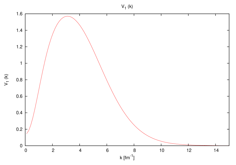
Figure 1: $V_{1}(k)$.

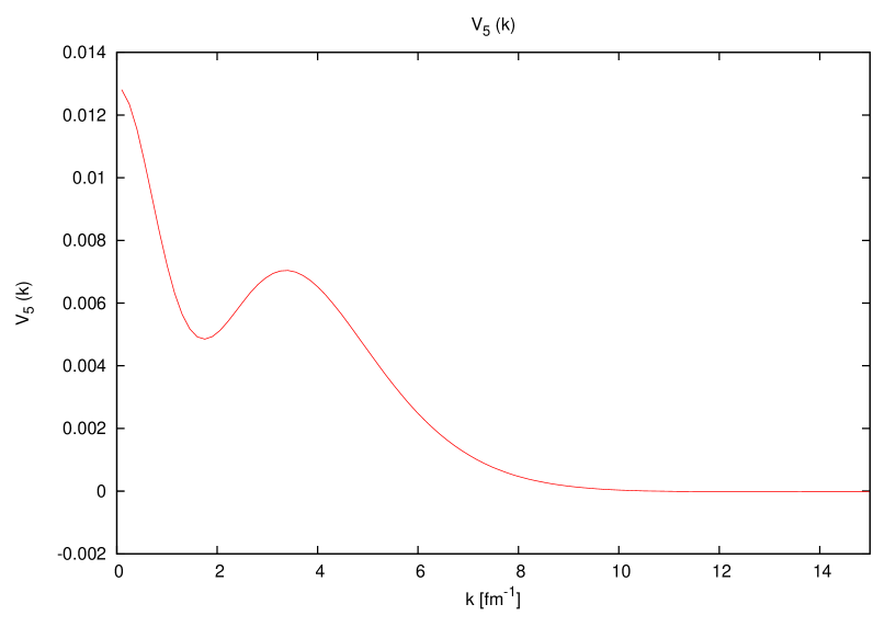
Figure 2: $V_{5}(k)$.

Figures 1 and 2 show the potential functions for the central and tensor parts ($V_{1}(q)$ and $V_{5}(q)$) of the interaction to illustrate the structure of typical potentials.

III.1 Chebyshev expansions

This section discusses the Chebyshev basis. The functions $\tilde{V}_{m}(q)$ are replaced by a Chebyshev polynomial approximation on the interval $q\in[a,b]$ using broucke

$$\tilde{V}_{m}(q)\approx c_{0}/2+\sum_{n=1}^{100}c_{n}T_{n}(-{a+b\over b-a}+{2\over b-a}q)$$ (8)

where

$$T_{n}(x)=\cos(n\cos^{-1}(x)))$$ (9)

are Chebyshev polynomials and the coefficients $c_{n}$ are computed using a Clenshaw-Curtiss quadrature broucke :

$$c_{n}={2\over N}[{1\over 2}\tilde{V}_{m}(b)+\sum_{j=1}^{N-1}\tilde{V}_{m}({a+b\over 2}+{b-a\over 2}\cos(\pi j/N))\cos(nj\pi/N)+(-)^{n}{1\over 2}\tilde{V}_{m}(a)]$$ (10)

with $N=101$. The functions $\tilde{V}_{m}(q)$ are evaluated at the quadrature points $q_{j}:={a+b\over 2}+{b-a\over 2}\cos(\pi j/N)$ using the methods discussed above. This is repeated for $q$ in each of three intervals, $[a,b]=[0,10],[10,50],[50,100]$ and the 101 expansion coefficients associated with each of these three intervals are stored. The Chebyshev polynomials are computed using the recurrence relations

$$T_{n+1}(x)=2xT_{n}(x)-T_{n-1}(x),\qquad T_{0}(x)=1,\,T_{1}(x)=x.$$ (11)

For $q$ larger than 100 $fm^{-1}$ $\tilde{V}_{m}(q)$ is approximated by 0.

For the potentials $\tilde{V}_{4}(q)$, $\tilde{V}_{6}(q)$ and $\tilde{V}_{17}(q)$ it was necessary to add additional Chebyshev expansions intervals between zero and ten $fm^{-1}$. For $\tilde{V}_{4}(q)$ 21 polynomials were used on $[0,.2]fm^{-1}$, 31 polynomials were used on $[.2,.5]fm^{-1}$, 41 polynomials were used on $[.5,2.0]fm^{-1}$ and 71 polynomials were used on $[2.0,10.0]fm^{-1}$. For $\tilde{V}_{6}(q)$ 31 polynomials were used on $[0,.5]fm^{-1}$, 41 polynomials were used on $[.5,2.0]fm^{-1}$ and 41 polynomials were used on $[2.0,10.0]fm^{-1}$. Similarly for $\tilde{V}_{17}(q)$ 31 polynomials were used on $[0,1.0]fm^{-1}$, 51 polynomials were used on $[1.0,5.0]fm^{-1}$ and 51 polynomials were used on $[5.0,10.0]fm^{-1}$.

This method provides an accurate and efficient representation for computing a momentum space $V18$ interaction. One of the supplementary programs (chebyshev-argonne.c) uses this method to compute the 24 coefficient functions in Table 2.

III.2 Rational basis functions

While the method of the previous section gives accurate results, a more straightforward approach is to represent the potential directly as an expansion in basis functions that have analytic Fourier transforms. In order to represent the potential, each of the scalar potentials $\tilde{V}_{m}(q)$, is approximated by an expansion in known basis functions. A method to compute both the expansion coefficients and a recursion formula to compute basis functions are given below.

The functions $V_{m}(r)$, $rV_{m}(r)$, and $r^{2}V_{m}(r)$ that appear in the integrands of the integrals in Table 2 are expanded using an orthonormal set of radial functions that have analytic Fourier-Bessel transforms keister . These functions are associated Laguerre polynomials multiplied by decaying exponentials in configuration space. Their Fourier-Bessel transforms have power-law fall of in momentum space. In addition, they vanish at the origin in a manner that can be used to explicitly cancel the factors $1/q$ and $1/q^{2}$ that appear in the definitions of $\tilde{V}_{m}$ in Table 2. Both sets of basis functions can be generated efficiently using recursion relations. The cancellation of the factors $1/q$ and $1/q^{2}$ can be directly incorporated into the recursion that generates the momentum-space basis functions so the final expression for the potential does not require a special treatment for $q$ near $0$.

The radial basis functions for different values of $l$ are given below. The dimensionless parameter $x:=\Lambda r$ is used in the basis functions, where $\Lambda$ is a scale parameter that can be chosen to improve efficiency. The parameterization of the Argonne V18 interaction uses the value $\Lambda=7(fm)^{-1}$. The configuration-space basis functions are

$$\phi_{nl}(r)={1\over\sqrt{N_{nl}}}x^{l}L_{n}^{2l+2}(2x)e^{-x}$$ (12)

where

$$L_{n}^{\alpha}=\sum_{m=0}^{n}(-)^{m}\left(\begin{array}[]{c}n+\alpha\\ n-m\\ \end{array}\right){x^{m}\over m!}$$ (13)

and the normalization coefficient is

$$N_{nl}=\Lambda^{-3}({1\over 2})^{2l+3}{\Gamma(n+\alpha+1)\over n!}.$$ (14)

These functions satisfy the orthogonality relations

$$\int_{0}^{\infty}\phi_{nl}(r)\phi_{ml}(r)r^{2}dr=\delta_{mn}.$$ (15)

They have analytic Fourier-Bessel transforms given by

$$\tilde{\phi}_{nl}(q)=\sqrt{2\over\pi}\int_{0}^{\infty}j_{l}(qr)\phi_{nl}(r)r^{2}dr.$$ (16)

For $y=q/\Lambda$ the $\tilde{\phi}_{nl}(q)$ can be expressed in terms of Jacobi polynomials:

$$\tilde{\phi}_{nl}(q)={1\over\sqrt{\tilde{N}_{nl}}}{y^{l}\over(y^{2}+1)^{l+2}}P_{n}^{l+{3\over 2},l+{1\over 2}}({y^{2}-1\over y^{2}+1})$$ (17)

with normalization coefficient

$$\tilde{N}_{nl}={\Lambda^{3}\over 2(2n+2l+3)}{\Gamma(n+l+{5\over 2})\Gamma(n+l+{3\over 2})\over n!\Gamma(n+2l+3)}$$ (18)

and

$$P^{(\alpha,\beta)}_{n}(x)={\Gamma(\alpha+n+1)\over n!\Gamma(\alpha+\beta+n+1)}\sum_{m=0}^{n}\left(\begin{array}[]{c}n\\ m\end{array}\right){\Gamma(\alpha+\beta+n+m+1)\over 2^{m}\Gamma(\alpha+m+1)}(x-1)^{m}.$$ (19)

These functions satisfy the orthogonality relations

$$\int_{0}^{\infty}\tilde{\phi}_{nl}(q)\tilde{\phi}_{ml}(q)q^{2}dq=\delta_{mn}.$$ (20)

These basis functions can be generated by using the recursion formulas for the associated Laguerre functions and Jacobi polynomials

$$(n+1)L^{\alpha}_{n+1}(x)=(2n+\alpha+1-x)L^{\alpha}_{n+}(x)-(n+\alpha)L^{\alpha}_{n-1}(x)$$ (21)

and

$$2(n+1)(n+\alpha+\beta+1)(2n+\alpha+\beta)P_{n+1}^{(\alpha,\beta)}(x)=$$

$$[(2n+\alpha+\beta+1)(\alpha^{2}-\beta^{2})+x((2n+\alpha+\beta)(2n+\alpha+\beta+1)(2n+\alpha+\beta+2)]P_{n}^{(\alpha,\beta)}(x)$$

$$-2(n+\alpha)(n+\beta)(2n+\alpha+\beta+2)P_{n-1}^{(\alpha,\beta)}(x).$$ (22)

These recursion relations can be modified to incorporate the normalization constants (14) and (18) directly into the recursion. The recursion for the normalized radial basis functions with $(x=\Lambda r)$ is given by:

$$\phi_{0l}(r)={1\over\sqrt{(2l+1)!}}{1\over\sqrt{2^{2l+3}}}\Lambda^{3/2}x^{l}e^{-x}$$ (23)

$$\phi_{1l}(r)={2l+3-2x\over\sqrt{2l+3}}\phi_{0l}(r)$$ (24)

$$\phi_{nl}(r)={2n+1+2l-2x\over\sqrt{n+1+2l}\sqrt{n}}\phi_{n-1,l}(r)-\sqrt{{(n-1)(n+1+2l)\over n(n+2+2l)}}\phi_{n-2,l}(r).$$ (25)

Similarly, the normalized momentum-space basis functions with $(y=q/\Lambda)$ are generated by the recursion:

$$\tilde{\phi}_{0l}(q)=$$

$${1\over\sqrt{(2l+3)!}}{1\over\sqrt{\Lambda^{3}}}{1\over\sqrt{{1\over 2}\cdots{2l+3\over 2}}}{1\over\sqrt{{1\over 2}\cdots{2l+1\over 2}}}y^{l}{1\over(y^{2}+1)^{2l+2}}$$ (26)

$$\tilde{\phi}_{1l}(q)=({1\over 2}+(l+2){y^{2}-1\over y^{2}+1})\sqrt{{2l+5\over(l+2+{1\over 2})(l+1+{1\over 2})}}\tilde{\phi}_{0l}(q)$$ (27)

$$\tilde{\phi}_{nl}(q)=$$

$$\sqrt{{(2n+2l+3)n(n+2l+2)\over(2n+2l+1)(n+l+{3\over 2})(n+l+{1\over 2})}}$$

$$\times{(2n+2l+1)(2l+2)(y^{2}+1)+(2n+2l+1)(2n+2l)(2n+2l+2)(y^{2}-1)\over 2n(n+2l+2)(2n+2l)(y^{2}-1)}\tilde{\phi}_{n-1l}(q)$$

$$-\sqrt{{(2n+2l+3)(n-1)n(n+1+2l)(n+2l+2)\over(2n+2l-1)(n+l+{3\over 2})(n+l+{1\over 2})(n+l+{1\over 2})(n+l-{1\over 2})}}$$

$$\times{(n+l+{1\over 2})(n+l-{1\over 2})(2n+2l+2)\over(n)(n+2l+2)(2n+2l)}\tilde{\phi}_{n-1l}(q).$$ (28)

Replacing $\tilde{\phi}_{0l}(q)$ in (26) by $\hat{\phi}_{0l}(q):=\tilde{\phi}_{0l}(q)/q^{l}$ given by

$$\hat{\phi}_{0l}(q)=$$

$${1\over\sqrt{(2l+3)!}}{1\over\sqrt{\Lambda^{3}}}{1\over\sqrt{{1\over 2}\cdots{2l+3\over 2}}}{1\over\sqrt{{1\over 2}\cdots{2l+1\over 2}}}\Lambda^{-l}{1\over(y^{2}+1)^{2l+2}}$$ (29)

to start the recursion in equations (27)-(28) generates $\hat{\phi}_{nl}(q):=\tilde{\phi}_{nl}(q)/q^{l}$, which are well-behaved as $q\to 0$. Seventy expansion coefficients are used to construct the momentum-space potential for each value of $m$

$$c_{nm}={1\over 2\pi^{2}}\int_{0}^{\infty}\phi_{n0}(r)V_{m}(r)r^{2}dr\qquad m\in\{1,2,3,4,15,16,18\}$$ (30)

$$c_{nm}={1\over 2\pi^{2}}\int_{0}^{\infty}\phi_{n1}(r)V_{m}(r)r^{3}dr\qquad m\in\{7,8,9b,10b,11b,12b,13b,14b\}$$ (31)

$$c_{nm}={1\over 2\pi^{2}}\int_{0}^{\infty}\phi_{n2}(r)V_{m}(r)r^{4}dr\qquad m\in\{9a,10a,11a,12a,13a,14a\}$$ (32)

$$c_{nm}={1\over 2\pi^{2}}\int_{0}^{\infty}\phi_{n2}(r)V_{m}(r)r^{2}dr\qquad m\in\{5,6,17\}.$$ (33)

The integrals are approximated using an 80 point Gauss-Legendre quadrature between 0 and 10$fm$. The basis functions $\phi_{nl}(r)$ are generated using (23-25). The scale parameter in the recursion for $\phi_{nl}(r)$ is taken as $\Lambda=7fm^{-1}$.

The 70x24 expansion coefficients $c_{nm}$ are stored. The momentum-space potential functions are then given by

$$\tilde{V}_{m}(q)=\sum_{n=1}^{70}c_{nm}\hat{\phi}_{nl}(q)$$ (34)

where the reduced expansion functions $\hat{\phi}_{nl}(q):=\tilde{\phi}_{nl}(q)/q^{l}$ are generated recursively using (27-29).

The full momentum-space potential in operator form is given by

$$V=\sum_{m\in S}\tilde{V}_{m}(q)\tilde{O}_{m}$$ (35)

where $\tilde{O}_{m}$ are the 24 operators in Table 3 and $q=\sqrt{k^{2}+k^{\prime 2}-2\mathbf{k}^{\prime}\cdot\mathbf{k}}$.

One of the supplementary programs (rational-argonne.c) uses this method to compute the 24 coefficient functions in Table 2.

IV Tests

Two tests are performed on the potentials. First, the momentum-space coefficient functions, $\tilde{V}_{m}(q)$, computed using the accurate numerical Fourier Bessel transforms, the Chebyshev expansion and the rational basis function expansion are compared. For the second test both representations of potential are used to compute the deuteron binding energy and wave functions. These results are compared to a direct calculation of these quantities using the partial-wave expansion of the original configuration space potential.

The results of the first test are shown in Tables 4-7, which list values of the Fourier-Bessel transforms of the 24 radial functions computed using these three different methods for momentum transfers of 1,5,15 and 25 $fm^{-1}$.

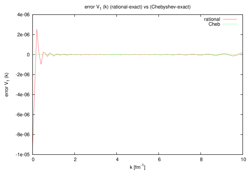
Figure 3: $\Delta V_{1\,rational}(k),\,\Delta V_{1\,Chebyshev}(k)$.

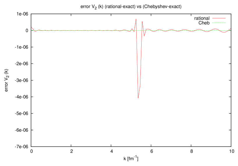
Figure 4: $\Delta V_{2\,rational}(k),\,\Delta V_{2\,Chebyshev}(k)$.

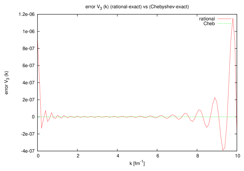
Figure 5: $\Delta V_{3\,rational}(k),\,\Delta V_{3\,Chebyshev}(k)$.

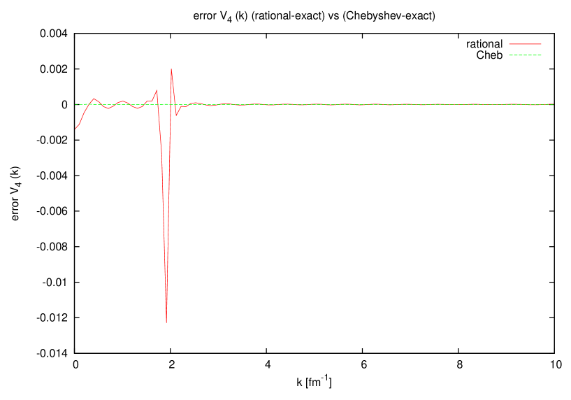
Figure 6: $\Delta V_{4\,rational}(k),\,\Delta V_{4\,Chebyshev}(k)$.

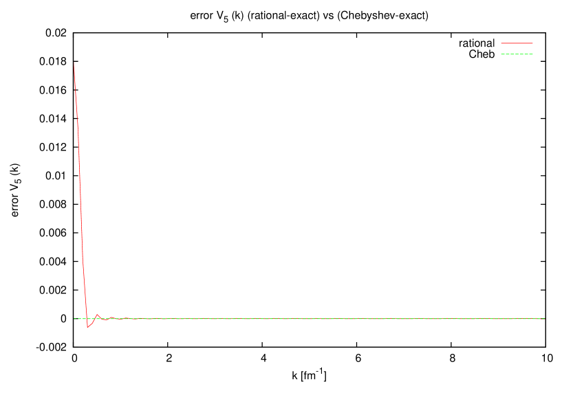
Figure 7: $\Delta V_{5\,rational}(k),\,\Delta V_{5\,Chebyshev}(k)$.

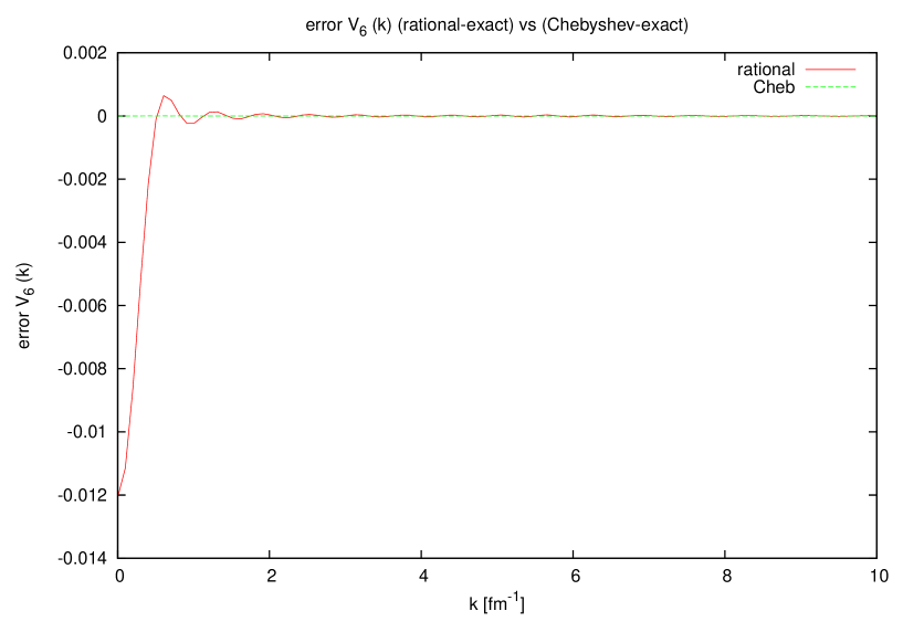
Figure 8: $\Delta V_{6\,rational}(k),\,\Delta V_{6\,Chebyshev}(k)$.

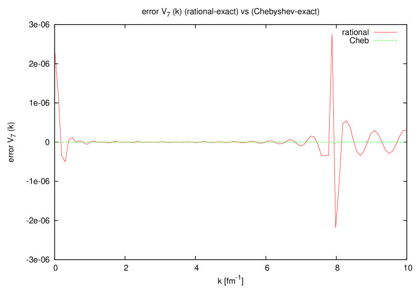
Figure 9: $\Delta V_{7\,rational}(k),\,\Delta V_{7\,Chebyshev}(k)$.

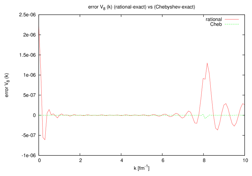
Figure 10: $\Delta V_{8\,rational}(k),\,\Delta V_{8\,Chebyshev}(k)$.

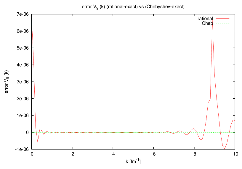
Figure 11: $\Delta V_{9b\,rational}(k),\,\Delta V_{9b\,Chebyshev}(k)$.

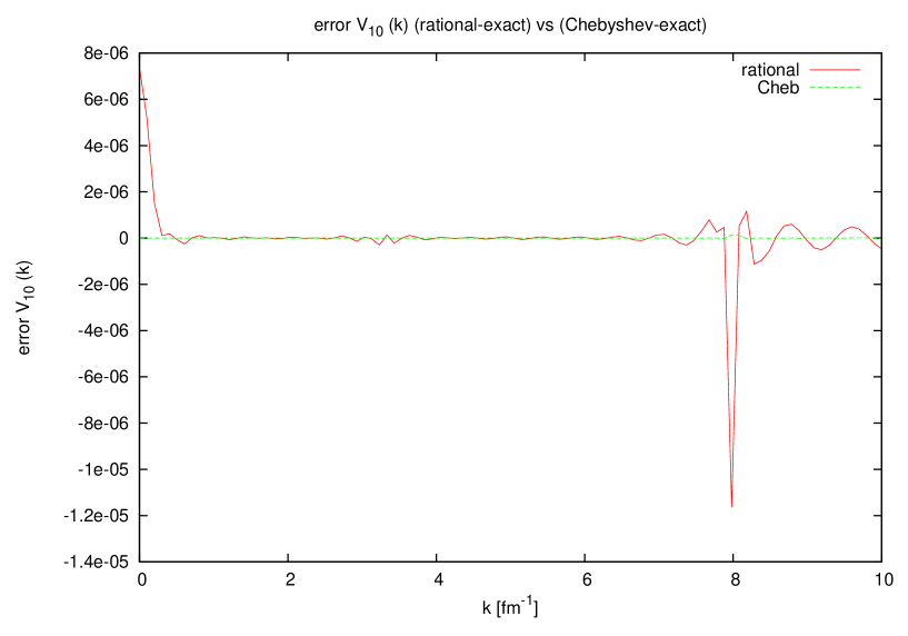
Figure 12: $\Delta V_{10b\,rational}(k),\,\Delta V_{10b\,Chebyshev}(k)$.

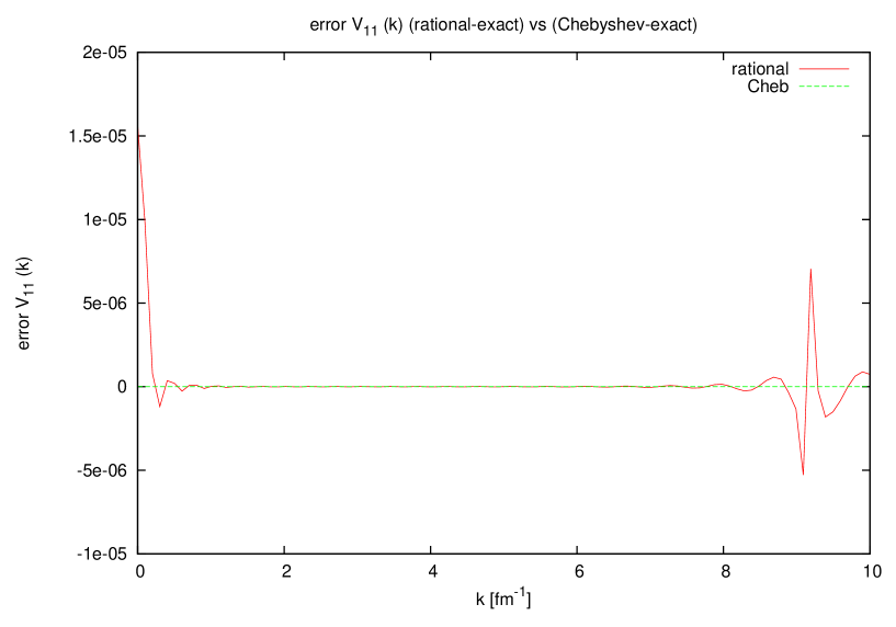
Figure 13: $\Delta V_{11b\,rational}(k),\,\Delta V_{11b\,Chebyshev}(k)$.

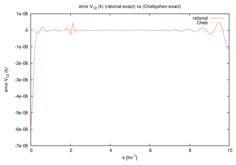
Figure 14: $\Delta V_{12b\,rational}(k),\,\Delta V_{12b\,Chebyshev}(k)$.

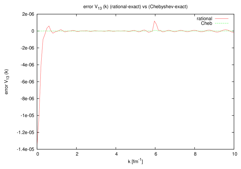
Figure 15: $\Delta V_{13b\,rational}(k),\,\Delta V_{13b\,Chebyshev}(k)$.

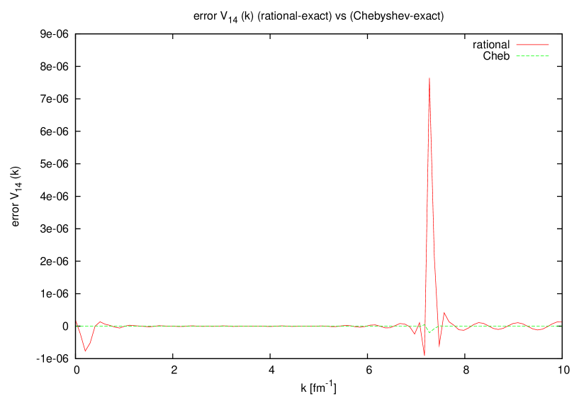
Figure 16: $\Delta V_{14b\,rational}(k),\,\Delta V_{14b\,Chebyshev}(k)$.

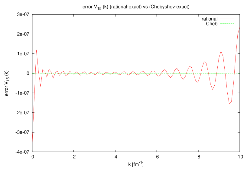
Figure 17: $\Delta V_{15\,rational}(k),\,\Delta V_{15\,Chebyshev}(k)$.

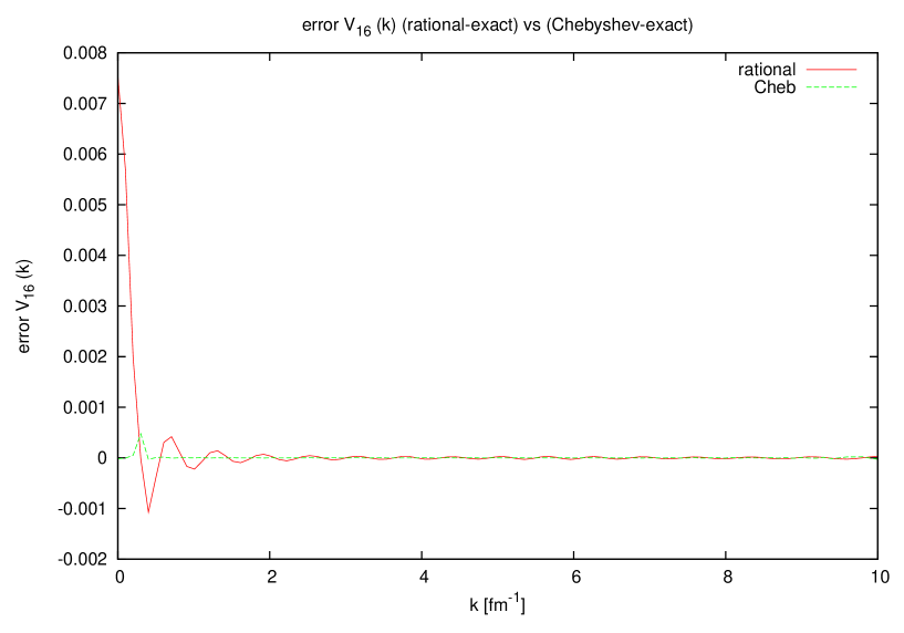
Figure 18: $\Delta V_{16\,rational}(k),\,\Delta V_{16\,Chebyshev}(k)$.

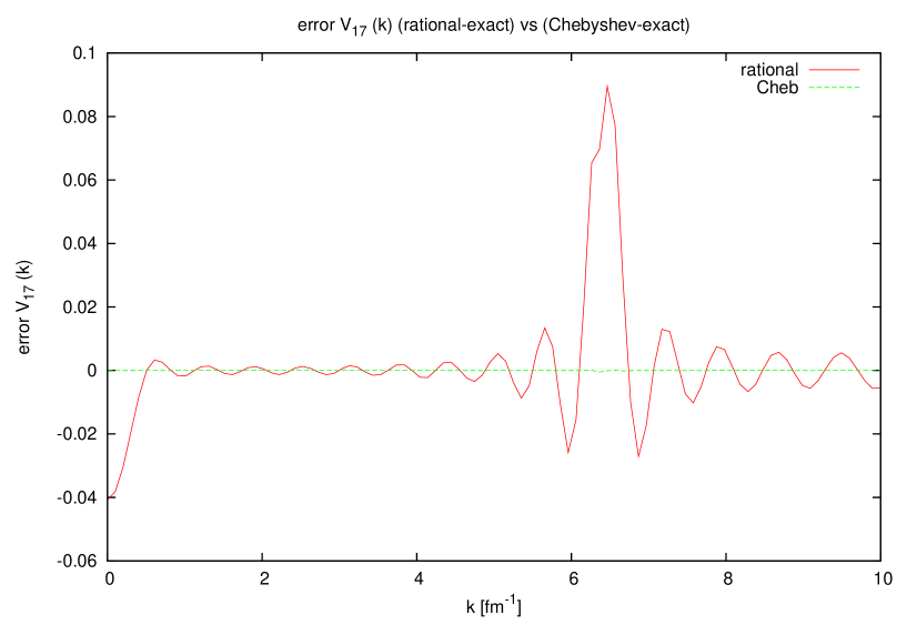
Figure 19: $\Delta V_{17\,rational}(k),\,\Delta V_{17\,Chebyshev}(k)$.

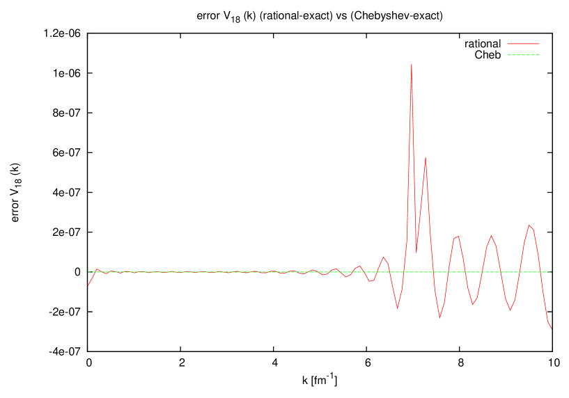
Figure 20: $\Delta V_{18\,rational}(k),\,\Delta V_{18\,Chebyshev}(k)$.

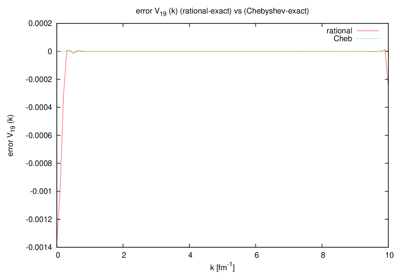
Figure 21: $\Delta V_{9a\,rational}(k),\,\Delta V_{9a\,Chebyshev}(k)$.

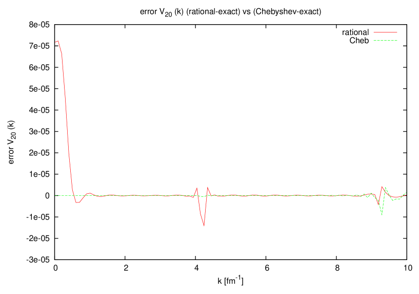
Figure 22: $\Delta V_{10a\,rational}(k),\,\Delta V_{10a\,Chebyshev}(k)$.

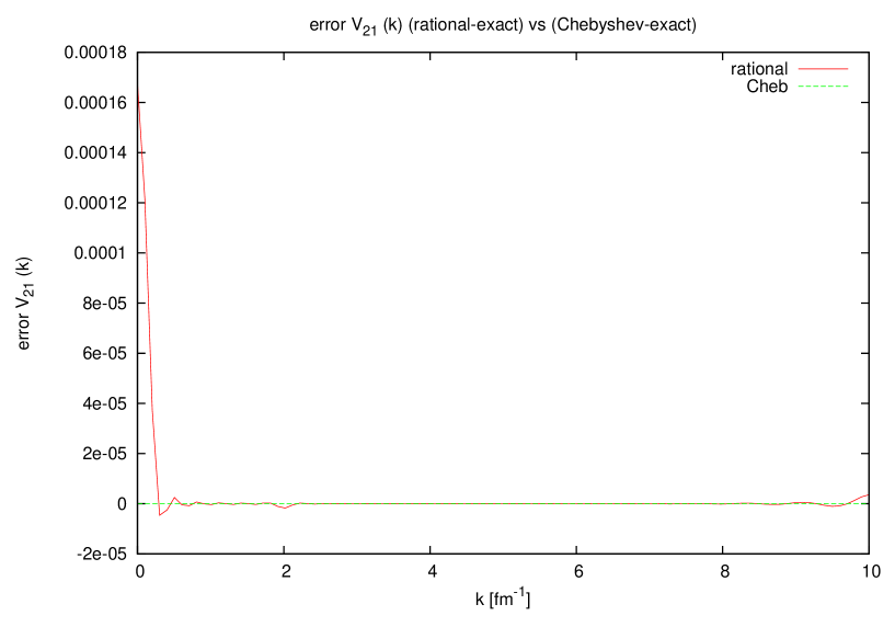
Figure 23: $\Delta V_{11a\,rational}(k),\,\Delta V_{11a\,Chebyshev}(k)$.

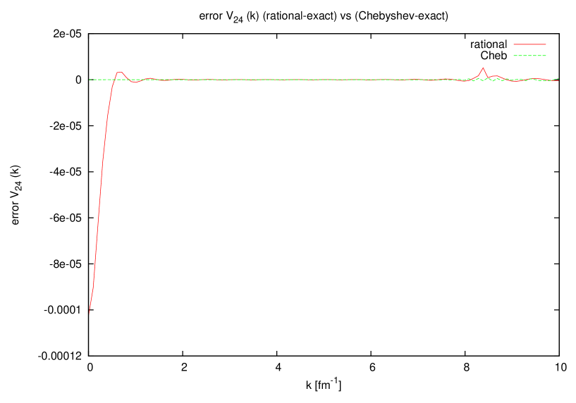
Figure 26: $\Delta V_{14a\,rational}(k),\,\Delta V_{14a\,Chebyshev}(k)$.

These results are shown in Tables 4,5,6 and 7 for all 24 operators and a representative range of the momentum transfers. The columns labeled RFExp show the scalar potential functions using the rational function expansion, the columns labeled CExp show the same quantities using the Chebyshev expansion, while the columns labeled NFT show the results of the direct numerical Fourier transform. Figures 3-26 plot the difference of the approximate Fourier transforms with an accurate Fourier Bessel transform divided by half of the sum of these quantities. The solid curves are for the rational function expansion and the dotted curved are for the Chebyshev expansion.

Table 4: Values of scalar coefficients at 1 fm^-1

n	RFExp	CExp	NFT
1	6.789973e-01	6.789977e-01	6.789977e-01
2	-4.019392e-01	-4.019392e-01	-4.019392e-01
3	-1.692090e-01	-1.692090e-01	-1.692090e-01
4	2.358519e-01	2.356704e-01	2.356705e-01
5	7.216739e-03	7.218217e-03	7.218217e-03
6	2.857732e-01	2.860471e-01	2.860467e-01
7	-5.511547e-01	-5.511547e-01	-5.511547e-01
8	-1.678888e-01	-1.678888e-01	-1.678888e-01
9	1.741415e-01	1.741415e-01	1.741415e-01
10	-3.272988e-02	-3.272987e-02	-3.272987e-02
11	1.999136e-02	1.999136e-02	1.999136e-02
12	-7.414060e-03	-7.414060e-03	-7.414060e-03
13	9.084422e-02	9.084424e-02	9.084424e-02
14	1.245017e-01	1.245017e-01	1.245017e-01
15	1.122388e-02	1.122389e-02	1.122389e-02
16	-1.214926e-02	-1.216021e-02	-1.216031e-02
17	2.403290e-03	2.420818e-03	2.420818e-03
18	6.124964e-03	6.124964e-03	6.124964e-03
19	1.304278e-02	1.304274e-02	1.304274e-02
20	-1.702409e-02	-1.702401e-02	-1.702401e-02
21	-7.227244e-03	-7.227256e-03	-7.227256e-03
22	-7.849686e-03	-7.849707e-03	-7.849707e-03
23	4.518193e-02	4.518262e-02	4.518262e-02
24	3.980251e-02	3.980269e-02	3.980269e-02

Table 5: Value of scalar coefficients at 5 fm^-1

n	RFExp	CExp	NFT
1	1.160699e+00	1.160699e-00	1.160699e-00
2	-1.360382e-02	-1.360382e-02	-1.360382e-02
3	-1.148807e-01	-1.148807e-01	-1.148807e-01
4	-1.065288e-01	-1.065203e-01	-1.065203e-01
5	4.489757e-03	4.489763e-03	4.489763e-03
6	4.405849e-03	4.405371e-03	4.405370e-03
7	-4.623736e-02	-4.623736e-02	-4.623736e-02
8	-1.871380e-02	-1.871380e-02	-1.871380e-02
9	2.471311e-02	2.471311e-02	2.471311e-02
10	1.480758e-03	1.480758e-03	1.480758e-03
11	6.027203e-03	6.027203e-03	6.027203e-03
12	1.465070e-03	1.465070e-03	1.465070e-03
13	5.222260e-03	5.222260e-03	5.222260e-03
14	8.233502e-03	8.233502e-03	8.233502e-03
15	4.828280e-03	4.828280e-03	4.828280e-03
16	-4.815794e-03	-4.815305e-03	-4.815305e-03
17	1.656921e-06	1.627533e-06	1.627533e-06
18	4.274306e-04	4.274306e-04	4.274306e-04
19	4.273833e-03	4.273832e-03	4.273832e-03
20	1.791462e-04	1.791461e-04	1.791461e-04
21	9.672551e-04	9.672550e-04	9.672550e-04
22	1.814761e-04	1.814761e-04	1.814761e-04
23	1.620319e-03	1.620318e-03	1.620318e-03
24	1.790086e-03	1.790085e-03	1.790085e-03

Table 6: Value of scalar coefficients at 15 fm^-1

n	RFExp	CExp	NFT
1	9.321365e-04	9.321031e-04	9.321031e-04
2	4.123439e-05	4.123387e-05	4.123387e-05
3	-1.924812e-05	-1.924669e-05	-1.924669e-05
4	-6.648375e-05	-6.643904e-05	-6.643770e-05
5	-9.010902e-06	-9.010512e-06	-9.010512e-06
6	1.026393e-05	1.026324e-05	1.026323e-05
7	5.541260e-06	5.540856e-06	5.540856e-06
8	2.632043e-06	2.631901e-06	2.631901e-06
9	-1.962835e-06	-1.962585e-06	-1.962585e-06
10	-9.304609e-07	-9.304846e-07	-9.304846e-07
11	-6.015901e-07	-6.015363e-07	-6.015363e-07
12	-1.047669e-07	-1.047529e-07	-1.047529e-07
13	-4.725022e-06	-4.725152e-06	-4.725152e-06
14	-1.527634e-06	-1.527584e-06	-1.527584e-06
15	2.942747e-06	2.942623e-06	2.942623e-06
16	-2.895027e-06	-2.892432e-06	-2.892244e-06
17	-2.865458e-10	-3.049671e-10	-3.061292e-10
18	9.986465e-08	9.985107e-08	9.985107e-08
19	-2.604487e-07	-2.604660e-07	-2.604660e-07
20	-6.335039e-08	-6.334951e-08	-6.334951e-08
21	-7.055132e-08	-7.055521e-08	-7.055521e-08
22	-1.454468e-08	-1.454569e-08	-1.454569e-08
23	-3.115148e-07	-3.115089e-07	-3.115089e-07
24	-1.394089e-07	-1.394129e-07	-1.394129e-07

Table 7: Value of scalar coefficients at 25 fm^-1

n	RFExp	CExp	NFT
1	-1.386301e-05	-1.383431e-05	-1.383431e-05
2	-6.108349e-08	-6.010007e-08	-6.010007e-08
3	8.598072e-07	8.595154e-07	8.595154e-07
4	1.014189e-06	1.003839e-06	1.003915e-06
5	-4.600082e-07	-4.599210e-07	-4.599210e-07
6	4.739733e-07	4.738710e-07	4.738711e-07
7	2.443040e-08	2.442088e-08	2.442088e-08
8	9.428095e-09	9.412965e-09	9.412965e-09
9	-1.534834e-08	-1.533919e-08	-1.533919e-08
10	3.457372e-10	3.607579e-10	3.607579e-10
11	-3.619628e-09	-3.613201e-09	-3.613201e-09
12	-1.005784e-09	-1.003137e-09	-1.003137e-09
13	4.666338e-09	4.709390e-09	4.709390e-09
14	-3.274714e-09	-3.270324e-09	-3.270324e-09
15	-5.425469e-08	-5.415686e-08	-5.415686e-08
16	5.452722e-08	5.398602e-08	5.399643e-08
17	-2.888773e-12	-4.263050e-12	-4.213031e-12
18	-5.852151e-09	-5.841440e-09	-5.841440e-09
19	-2.512190e-10	-2.555613e-10	-2.555613e-10
20	7.827015e-12	7.411785e-12	7.411785e-12
21	-5.864134e-11	-5.980761e-11	-5.980761e-11
22	-1.617550e-11	-1.652711e-11	-1.652711e-11
23	8.297311e-11	8.271942e-11	8.271943e-11
24	-5.322500e-11	-5.424546e-11	-5.424546e-11

These tables show generally good agreement among the three methods of computation. At 1$fm^{-1}$ and 5$fm^{-1}$ the Chebyshev expansion agrees with the direct numerical Fourier transform to between 5-7 significant figures for all 24 potentials. There is similar agreement at 15$fm^{-1}$ and 25$fm^{-1}$ except in potentials 17. The agreement between the potentials calculated using the rational function expansion do not agree with the direct numerical Fourier transforms as well as the Chebyshev expansion. The accuracy depends on the particular potential and gets worse as the momentum transfer increases. Thus for precision calculations the Chebyshev expansion is preferred.

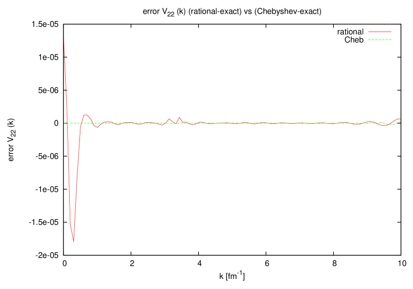
Figure 24: $\Delta V_{12a\,rational}(k),\,\Delta V_{12a\,Chebyshev}(k)$.

Figures 1-24 provide a more complete picture of the nature of the errors in both approximations. Spikes in the errors occur near points where the potentials change sign. Some of the errors near zero are enhanced because the some of the plotted potential are divided by powers of the momentum transfer. For these terms the operators include compensating powers of the momentum transfer that vanish near the origin, so the contribution of the error in the full potential near the origin is reduced. The rational function expansions have larger relative errors near higher and lower values of the momentum transfer. This is not surprising because the basis functions are not local. The Chebyshev expansion is uniformly good, in part because it is a local expansion, so more intervals can be added as needed. The largest errors are in potential 17. At $10fm^{-1}$ its value is about $-1.2\times 10^{-8}$, which is several orders of magnitude smaller than any of the other potentials at that momentum transfer.

Table 8: deuteron $s$ and $d$ wave functions using Chebyshev expansion,

rational function expansion and $r$-space partial waves

k$fm^{-1}$	$u_{s}(k)$-CExp.	$u_{s}(k)$-RFExp	$u_{s}(k)$-pw	$u_{d}(k)$-CExp,	$u_{d}(k)$-RFExp	$u_{d}(k)$-pw
0.0	1.2695e+01	1.2695e+01	1.2693e+01	0.00000e+00	0.00000e+00	0.00000e+00
0.5	1.9609e+00	1.9609e+00	1.9609e+00	-2.19827e-01	-2.19811e-01	-2.19826e-01
1.0	3.7684e-01	3.7685e-01	3.7684e-01	-1.72164e-01	-1.72159e-01	-1.72164e-01
1.5	8.2472e-02	8.2472e-02	8.2471e-02	-1.12429e-01	-1.12429e-01	-1.12429e-01
2.0	6.0809e-03	6.0808e-03	6.0806e-03	-7.10857e-02	-7.10863e-02	-7.10857e-02
2.5	-1.3615e-02	-1.3616e-02	-1.3615e-02	-4.45428e-02	-4.45432e-02	-4.45428e-02
3.0	-1.6153e-02	-1.6153e-02	-1.6153e-02	-2.76853e-02	-2.76854e-01	-2.76853e-02
3.5	-1.3648e-02	-1.3648e-02	-1.3648e-02	-1.69880e-02	-1.69881e-02	-1.69881e-02
4.0	-1.0153e-02	-1.0153e-02	-1.0153e-02	-1.02233e-02	-1.02234e-02	-1.02234e-02
4.5	-6.9954e-03	-6.9954e-03	-6.9953e-03	-5.98472e-03	-5.98475e-03	-5.98472e-03
5.0	-4.5270e-03	-4.5270e-03	-4.5270e-03	-3.37040e-03	-3.37043e-03	-3.37041e-03

As a second test the deuteron binding energy and wave functions are computed using the two different momentum-space potentials are compared to each other and to the direct Fourier transform of wave functions computed using a configuration-space partial-wave calculation.

The deuteron binding energy and the $s$ and $d$ wave functions are computed using the operator form of the Fourier transformed potential, by direct integration of the vector variables. The method of solution, which is discussed in charlotte , uses the expansion (7) directly without using partial waves. Calculations are performed for both the Chebyshev and rational-function representations of the momentum space potentials.

These calculations are compared to a configuration-space partial-wave calculation. In that calculation, labeled $pw$ in table 9, the wave functions are represented by an expansion in 70 configuration-space basis functions using the configuration-space basis functions (12). Matrix elements of the partial wave projection of the Hamiltonian, with the configuration space Argonne V18 potential, are computed in this basis and the eigenvalue problem is solved numerically. The Fourier transform is computed by analytically Fourier transforming the basis functions. The solution of the eigenvalue problem gives an independent evaluation of both the binding energy and wave functions constructed directly from the configuration space potential.

The deuteron binding energy obtained using the Chebyshev representation of the Fourier transform gives a deuteron binding energy of $E_{d}=-2.242233$ MeV. The rational function representation gives a d deuteron binding energy of $E_{d}=-2.242193$ MeV compared with $E_{d}=-2.242211$ MeV using the configuration space partial-wave calculation. The binding energies based on all three calculation agree to within 22 eV. The computation used in the configuration-space partial-wave calculation is a Galerkin calculation and thus gives a variational bound on the binding energy.

These eigenvalues differ from the experimental deuteron binding energy. This is because the momentum-space potentials used in these computations do not include electromagnetic corrections that appear in the Argonne V18 codes. The electromagnetic corrections contribute an additional $+17.6$ keV wiringa to the binding energy which is consistent with the experimental binding energy of $-2.2246$ MeV.

The $s$ and $d$ wave functions for all three calculations are compared in Table 10. The wave functions differ in the fifth or sixth significant figure, while binding energies of all three calculations differ in the sixth significant figure.

The electromagnetic contributions to the Argonne V18 potential are important for low-energy high-precision calculations. The Fourier transform of the electromagnetic contributions of the Argonne V18 potential can be computed analytically, and can be added to the strong interaction contribution discussed in this paper when necessary. The analytic Fourier transform of the electromagnetic contribution is discussed in appendix 3.

While this paper gives the momentum-space version of the operator expansion of the Argonne V18 potential, it is often useful to have partial-wave contributions of the potential. These can be computed from the operator matrix elements using a one-dimensional integration over the cosine of the angle between the initial and final momenta. A simple method to compute the partial-wave projections from the operator expansion is given in the appendix 2.

The programs to compute the potentials $\tilde{V}_{m}(q)$ using both methods are available as supplementary material to the electronic version of this article.

This work supported by the U.S. Department of Energy, contract # DE-FG02-86ER40286 and National Science Foundation grants NSF-PHY-1005578 and NSF-PHY-1005501. The authors would like to acknowledge useful comments from Prof. C. Elster in preparing this manuscript.

V Appendix 1

In this appendix we compute the Fourier transform of the parts of the potential containing the five types of operators, $\mathbf{I}$, $\mathbf{L}\cdot\mathbf{S}$, $\mathbf{L}\cdot\mathbf{L}$,$(\mathbf{L}\cdot\mathbf{S})^{2}$, and $S_{12}$ that appear in equations(3-6).

$\mathbf{L}\cdot\mathbf{S}$:

Let $\mathbf{q}:=\mathbf{k}^{\prime}-\mathbf{k}$.

The Fourier transform is

$${1\over(2\pi)^{3}}\int e^{-i\mathbf{k}^{\prime}\cdot\mathbf{r}}V_{j}(r)\mathbf{L}\cdot\mathbf{S}e^{i\mathbf{k}\cdot\mathbf{r}}d\mathbf{r}={1\over(2\pi)^{3}}\int e^{-i\mathbf{k}^{\prime}\cdot\mathbf{r}}V_{j}(r)\mathbf{S}\cdot(\mathbf{r}\times\mathbf{p})e^{i\mathbf{k}\cdot\mathbf{r}}d\mathbf{r}=$$

$${1\over(2\pi)^{3}}\int e^{-i\mathbf{k}^{\prime}\cdot\mathbf{r}}V_{j}(r)\mathbf{S}\cdot(\mathbf{r}\times\mathbf{k})e^{i\mathbf{k}\cdot\mathbf{r}}d\mathbf{r}={1\over(2\pi)^{3}}\int e^{-i\mathbf{q}\cdot\mathbf{r}}V_{j}(r)\mathbf{S}\cdot(\mathbf{r}\times\mathbf{k})d\mathbf{r}=$$

$${4\pi\over(2\pi)^{3}}\int\sum_{l=0}^{\infty}\sum_{m=-l}^{l}(-i)^{l}j_{l}(qr)Y_{lm}(\hat{\mathbf{q}})Y_{lm}^{*}(\hat{\mathbf{r}})V_{j}(r)\mathbf{S}\cdot(\mathbf{r}\times\mathbf{k})d\mathbf{r}.$$ (36)

Since $\mathbf{r}$ can be expanded as a linear combination of spherical harmonics, $Y_{1m}(\hat{\mathbf{r}})$, the only terms that survive are the $l=1$ terms. The integral over angles and the spherical harmonics replace $\hat{\mathbf{r}}$ by $\hat{\mathbf{q}}$, giving

$$-{4\pi i\over(2\pi)^{3}}\int_{0}^{\infty}j_{1}(qr)V_{j}(r)\mathbf{S}\cdot(\mathbf{q}\times\mathbf{k})r^{3}dr=$$

$$i\mathbf{S}\cdot(\mathbf{k}\times\mathbf{k}^{\prime})\times[{1\over 2\pi^{2}q}\int_{0}^{\infty}j_{1}(qr)V_{j}(r)r^{3}dr].$$ (37)

Thus the Fourier transform has the form

$${1\over(2\pi)^{3}}\int e^{-i\mathbf{k}^{\prime}\cdot\mathbf{r}}V_{j}(r)\mathbf{L}\cdot\mathbf{S}e^{i\mathbf{k}\cdot\mathbf{r}}d\mathbf{r}=i\mathbf{S}\cdot(\mathbf{k}\times\mathbf{k}^{\prime})I_{1}(q)$$ (38)

where

$$I_{1}(q):={1\over 2\pi^{2}q}\int_{0}^{\infty}j_{1}(qr)V_{j}(r)r^{3}dr.$$ (39)

The following relations are used to compute Fourier transforms of the remaining three operators:

$$\boldsymbol{\nabla}_{q}f(q)=f^{\prime}(q){\mathbf{q}\over q}$$ (40)

$$\nabla_{q}^{2}f(q)=f^{\prime\prime}(q)+{2\over q}f^{\prime}(q)$$ (41)

$$(\mathbf{a}\cdot\boldsymbol{\nabla}_{q})(\mathbf{b}\cdot\boldsymbol{\nabla}_{q})f(q)=$$

$${\mathbf{a}\cdot\mathbf{q}\over q}{\mathbf{b}\cdot\mathbf{q}\over q}(f^{\prime\prime}(q)-{f^{\prime}(q)\over q})+{\mathbf{a}\cdot\mathbf{b}\over q}f^{\prime}(q).$$ (42)

$\mathbf{L}\cdot\mathbf{L}$:

The Fourier transform of this operator is

$${1\over(2\pi)^{3}}\int e^{-i\mathbf{k}^{\prime}\cdot\mathbf{r}}V_{j}(r)(\mathbf{r}\times\mathbf{p})\cdot(\mathbf{r}\times\mathbf{p})e^{i\mathbf{k}\cdot\mathbf{r}}d\mathbf{r}={1\over(2\pi)^{3}}\int e^{-i\mathbf{k}^{\prime}\cdot\mathbf{r}}V_{j}(r)(\mathbf{r}\times\mathbf{k}^{\prime})\cdot(\mathbf{r}\times\mathbf{k})e^{i\mathbf{k}\cdot\mathbf{r}}d\mathbf{r}=$$

$$(i\boldsymbol{\nabla}_{q}\times\mathbf{k}^{\prime})\cdot(i\boldsymbol{\nabla}_{q}\times\mathbf{k}){1\over(2\pi)^{3}}\int V_{j}(r)e^{-i\mathbf{q}\cdot\mathbf{r}}d\mathbf{r}=-(\boldsymbol{\nabla}_{q}\times\mathbf{k}^{\prime})\cdot(\boldsymbol{\nabla}_{q}\times\mathbf{k}){4\pi\over(2\pi)^{3}}\int_{0}^{\infty}V_{j}(r)j_{0}(qr)r^{2}dr.$$ (43)

To compute the derivatives use

$$(\boldsymbol{\nabla}_{q}\times\mathbf{k}^{\prime})\cdot(\boldsymbol{\nabla}_{q}\times\mathbf{k})=(\mathbf{k}\cdot\mathbf{k}^{\prime})(\boldsymbol{\nabla}_{q}\cdot\boldsymbol{\nabla}_{q})-(\mathbf{k}\cdot\boldsymbol{\nabla}_{q})(\mathbf{k}\cdot\boldsymbol{\nabla}_{q})$$

in the above to get

$$-(\boldsymbol{\nabla}_{q}\times\mathbf{k}^{\prime})\cdot(\boldsymbol{\nabla}_{q}\times\mathbf{k}){4\pi\over(2\pi)^{3}}\int_{0}^{\infty}V_{j}(r)j_{0}(qr)r^{2}dr=-\left((\mathbf{k}^{\prime}\cdot\mathbf{k})\nabla^{2}_{q}-(\mathbf{k}^{\prime}\cdot\boldsymbol{\nabla}_{q})(\mathbf{k}\cdot\boldsymbol{\nabla}_{q})\right)I_{0}(q)$$ (44)

where

$$I_{0}(q)={4\pi\over(2\pi)^{3}}\int_{0}^{\infty}V_{j}(r)j_{0}(qr)r^{2}dr={1\over 2\pi^{2}}\int_{0}^{\infty}V_{j}(r)j_{0}(qr)r^{2}dr.$$ (45)

Evaluating this gives

$$-\left((\mathbf{k}^{\prime}\cdot\mathbf{k})\nabla^{2}_{q}-(\mathbf{k}^{\prime}\cdot\boldsymbol{\nabla}_{q})(\mathbf{k}\cdot\boldsymbol{\nabla}_{q})\right)I_{0}(q)=$$

$$-(\mathbf{k}^{\prime}\cdot\mathbf{k})(I_{0}^{\prime\prime}(q)+{1\over q}I_{0}^{\prime}(q))+{(\mathbf{k}^{\prime}\cdot\mathbf{q})(\mathbf{k}\cdot\mathbf{q})\over q^{2}}(I_{0}^{\prime\prime}(q)-{1\over q}I_{0}^{\prime}(q)).$$ (46)

To eliminate the derivatives use

$$I_{0}^{\prime\prime}(q)-{1\over q}I_{0}^{\prime}(q)=$$

$${1\over 2\pi^{2}}\int_{0}^{\infty}V(r)(j_{0}^{\prime\prime}(qr)-j_{0}^{\prime}(qr){1\over qr})r^{4}dr={1\over 2\pi^{2}}\int_{0}^{\infty}V(r)j_{2}(qr)r^{4}dr=I_{2}(q)$$

and

$$I_{0}^{\prime\prime}(q)+{1\over q}I_{0}^{\prime}(q)={1\over 2\pi^{2}}\int_{0}^{\infty}V(r)(j_{0}^{\prime\prime}(qr)-j_{0}^{\prime}(qr){1\over qr}+2j_{0}^{\prime}(qr){1\over qr})r^{4}dr=$$

$${1\over 2\pi^{2}}\int_{0}^{\infty}V(r)j_{2}^{\prime\prime}(qr)r^{4}dr-{1\over 2\pi^{2}}{2\over q}\int_{0}^{\infty}V(r)j_{1}(qr)r^{3}dr=I_{2}(q)-{2\over q}I_{1}(q).$$

This gives

$${1\over(2\pi)^{3}}\int e^{-i\mathbf{k}^{\prime}\cdot\mathbf{r}}V_{j}(r)(\mathbf{r}\times\mathbf{p})\cdot(\mathbf{r}\times\mathbf{p})e^{i\mathbf{k}\cdot\mathbf{r}}d\mathbf{r}=-(\mathbf{k}^{\prime}\cdot\mathbf{k})(I_{2}(q)-{2\over q}I_{1}(q))+{(\mathbf{k}^{\prime}\cdot\mathbf{q})(\mathbf{k}\cdot\mathbf{q})\over q^{2}}I_{2}(q)$$ (47)

which can be reexpressed in terms of cross products:

$${1\over(2\pi)^{3}}\int e^{-i\mathbf{k}^{\prime}\cdot\mathbf{r}}V_{j}(r)(\mathbf{r}\times\mathbf{p})\cdot(\mathbf{r}\times\mathbf{p})e^{i\mathbf{k}\cdot\mathbf{r}}d\mathbf{r}=-I_{2}(q){(\mathbf{k}^{\prime}\times\mathbf{k})\cdot(\mathbf{k}^{\prime}\times\mathbf{k})\over q^{2}}+{2\over q}(\mathbf{k}^{\prime}\cdot\mathbf{k})I_{1}(q).$$ (48)

$(\mathbf{L}\cdot\mathbf{S})^{2}$:

The Fourier transform is

$${1\over(2\pi)^{3}}\int e^{-i(\mathbf{k}^{\prime}-\mathbf{k})\cdot\mathbf{r}}V_{j}(r)(\mathbf{L}\cdot\mathbf{S})^{2}d\mathbf{r}={1\over(2\pi)^{3}}\int e^{-i(\mathbf{k}^{\prime}-\mathbf{k})\cdot\mathbf{r}}V_{j}(r)(\mathbf{S}\cdot(\mathbf{r}\times\mathbf{p}))^{2}d\mathbf{r}=$$

$$-{4\pi\over(2\pi)^{3}}((\mathbf{k}^{\prime}\times\mathbf{S})\cdot\boldsymbol{\nabla}_{q})((\mathbf{k}\times\mathbf{S})\cdot\boldsymbol{\nabla}_{q})\int j_{0}(qr)V_{j}(r)r^{2}dr=$$

$$-((\mathbf{k}^{\prime}\times\mathbf{S})\cdot\boldsymbol{\nabla}_{q})((\mathbf{k}\times\mathbf{S})\cdot\boldsymbol{\nabla}_{q})I_{0}(q)=$$

$$-((\mathbf{k}^{\prime}\times\mathbf{S})\cdot\mathbf{q}((\mathbf{k}\times\mathbf{S})\cdot\mathbf{q})){1\over q^{2}}(I_{0}^{\prime\prime}(q)-{1\over q}I^{\prime}_{0}(q))-(\mathbf{k}^{\prime}\times\mathbf{S})\cdot(\mathbf{k}\times\mathbf{S}){1\over q}I^{\prime}_{0}(q)=$$

$$-((\mathbf{k}^{\prime}\times\mathbf{S})\cdot\mathbf{q}((\mathbf{k}\times\mathbf{S})\cdot\mathbf{q}))={1\over q^{2}}I_{2}(q)+(\mathbf{k}^{\prime}\times\mathbf{S})\cdot(\mathbf{k}\times\mathbf{S}){1\over q}I_{1}(q)$$ (49)

which gives

$$-((\mathbf{S}\cdot(\mathbf{k}\times\mathbf{k}^{\prime}))^{2}{1\over q^{2}}I_{2}(q)+(\mathbf{k}^{\prime}\times\mathbf{S})\cdot(\mathbf{k}\times\mathbf{S}){1\over q}I_{1}(q)$$ (50)

or

$${1\over(2\pi)^{2}}\int e^{-i(\mathbf{k}^{\prime}-\mathbf{k})}V_{j}(r)(\mathbf{L}\cdot\mathbf{S})^{2}d\mathbf{r}=-((\mathbf{S}\cdot(\mathbf{k}\times\mathbf{k}^{\prime}))^{2}{1\over q^{2}}I_{2}(q)+(\mathbf{k}^{\prime}\times\mathbf{S})\cdot(\mathbf{k}\times\mathbf{S}){1\over q}I_{1}(q).$$ (51)

${1\over 3}S_{12}=\left(\hat{\mathbf{r}}\cdot\boldsymbol{\sigma}_{1})(\hat{\mathbf{r}}\cdot\boldsymbol{\sigma}_{2})-{1\over 3}\boldsymbol{\sigma}_{1}\cdot\boldsymbol{\sigma}_{2}\right)$:

The Fourier transform is

$${1\over(2\pi)^{3}}\int e^{-i\mathbf{k}^{\prime}\cdot\mathbf{r}}V(r)\left((\hat{\mathbf{r}}\cdot\boldsymbol{\sigma}_{1})(\hat{\mathbf{r}}\cdot\boldsymbol{\sigma}_{2})-{1\over 3}\boldsymbol{\sigma}_{1}\cdot\boldsymbol{\sigma}_{2}\right)e^{i\mathbf{k}\cdot\mathbf{r}}d\mathbf{r}=$$

$$-\left((\boldsymbol{\nabla}_{q}\cdot\boldsymbol{\sigma}_{1})(\boldsymbol{\nabla}_{q}\cdot\boldsymbol{\sigma}_{2})-{1\over 3}\boldsymbol{\sigma}_{1}\cdot\boldsymbol{\sigma}_{2}\boldsymbol{\nabla}_{q}^{2}\right){4\pi\over(2\pi)^{3}}\int V(r){r^{2}\over r^{2}}j_{0}(qr)dr=$$

$$-{\boldsymbol{\sigma}_{1}\cdot\mathbf{q}\over q}{\boldsymbol{\sigma}_{2}\cdot\mathbf{q}\over q}((I_{0-}^{\prime\prime}(q)-{I_{0-}^{\prime}(q)\over q})-{\mathbf{s}_{1}\cdot\mathbf{s}_{2}\over q}I_{0}^{\prime}(q)=$$

$$+{1\over 3}\boldsymbol{\sigma}_{1}\cdot\boldsymbol{\sigma}_{2}(I^{\prime\prime}_{0-}(q)+{2\over q}I_{0-}^{\prime}(q))$$ (52)

Thus,

$${1\over(2\pi)^{3}}\int e^{-i\mathbf{k}^{\prime}\cdot\mathbf{r}}V(r)\left(3(\hat{\mathbf{r}}\cdot\boldsymbol{\sigma}_{1})(\hat{\mathbf{r}}\cdot\boldsymbol{\sigma}_{2})-\boldsymbol{\sigma}_{1}\cdot\boldsymbol{\sigma}_{2}\right)e^{i\mathbf{k}\cdot\mathbf{r}}d\mathbf{r}=-\left(3{\boldsymbol{\sigma}_{1}\cdot\mathbf{q}\over q}{\boldsymbol{\sigma}_{2}\cdot\mathbf{q}\over q}-\boldsymbol{\sigma}_{1}\cdot\boldsymbol{\sigma}_{2}\right)I_{2-}(q)$$ (53)

where

$$I_{0-}(q)={4\pi\over(2\pi)^{3}}\int V(r)j_{2}(qr)r^{2}dr.$$ (54)

VI Appendix 2

In this appendix we compute the partial-wave projection of potentials from the vector representation of the momentum-space potential. Using rotational invariance the partial-wave potentials can be expressed using a one-dimensional integral over the cosine of the angle between the initial and final momentum vectors. The method below is similar to the method first proposed in ce11 .

Rotational invariance of the potential implies

$$\langle j,\mu,k,l,s|V|j^{\prime},\mu^{\prime},k^{\prime},l^{\prime},s^{\prime}\rangle$$

$$=\langle j,\mu,k,l,s|U^{\dagger}(R)VU(R)|j^{\prime},\mu^{\prime},k^{\prime},l^{\prime},s^{\prime}\rangle$$

$$=\sum_{\nu\nu^{\prime}}D^{j*}_{\nu\mu}(R)D^{j}_{\nu^{\prime}\mu^{\prime}}(R)\langle j,\nu,k,l,s|V|j^{\prime},\nu^{\prime},k^{\prime},l^{\prime},s^{\prime}\rangle$$

$$=\int dR\sum_{\nu\nu^{\prime}}D^{j*}_{\nu\nu^{\prime}}(R)D^{j}_{\nu^{\prime}\mu^{\prime}}(R)\langle j,\nu,k,l,s|V|j^{\prime},\nu^{\prime},k^{\prime},l^{\prime},s^{\prime}\rangle$$

$$=\delta_{jj^{\prime}}\sum_{\mu^{\prime}\nu^{\prime}}\delta_{\mu\mu^{\prime}}{\delta_{\nu\nu^{\prime}}\over 2j+1}\langle j,\nu,k,l,s|V|j^{\prime},\nu^{\prime},k^{\prime},l^{\prime},s^{\prime}\rangle$$

$$=\delta_{\mu\mu^{\prime}}\delta_{jj^{\prime}}\langle k,l,s\|V^{j}\|k^{\prime},l^{\prime},s^{\prime}\rangle$$ (55)

where we have integrated over the $SU(2)$ Haar measure with normalization $\int dR=1$ and defined the partial-wave potentials by

$$\langle k,l,s\|V^{j}\|k^{\prime},l^{\prime},s^{\prime}\rangle:={1\over 2j+1}\sum_{\mu=-j}^{j}\sum_{m_{l}m_{l}^{\prime}}\sum_{m_{s}m_{s}^{\prime}}\langle j,\mu,k,l,s|V|j,\mu,k^{\prime},l^{\prime},s^{\prime}\rangle.$$ (56)

This kernel is rotationally invariant. Formally the partial-wave potential is

$$\langle k,l,s\|V^{j}\|k^{\prime},l^{\prime},s^{\prime}\rangle$$

$$=\int d\hat{\mathbf{k}}d\hat{\mathbf{k}}^{\prime}{1\over 2j+1}\sum_{\mu=-j}^{j}\langle{1\over 2},\mu_{1},{1\over 2},\mu_{2}|s,m_{s}\rangle\langle l,m_{l},s,m_{s}|j,\mu\rangle Y_{lm_{l}}^{*}(\hat{\mathbf{k}})$$

$$\times\langle\mathbf{k},\mu_{1},\mu_{2}\|V\|\mathbf{k}^{\prime},\mu_{1}^{\prime},\mu_{2}^{\prime}\rangle$$

$$\times\langle{1\over 2},\mu_{1}^{\prime},{1\over 2},\mu_{2}^{\prime}|s^{\prime},m_{s}^{\prime}\rangle\langle l^{\prime},m_{l}^{\prime},s^{\prime},m_{s}^{\prime}|j,\mu\rangle Y_{l^{\prime}m_{l}^{\prime}}(\hat{\mathbf{k}}^{\prime}).$$ (57)

For any fixed rotation, $R$, rotational invariance of $V$ gives

$$\langle\mathbf{k},\mu_{1},\mu_{2}\|V\|\mathbf{k}^{\prime},\mu_{1}^{\prime},\mu_{2}^{\prime}\rangle$$

$$=\langle\mathbf{k},\mu_{1},\mu_{2}\|U^{\dagger}(R)VU(R)\|\mathbf{k}^{\prime},\mu_{1}^{\prime},\mu_{2}^{\prime}\rangle$$

$$=\sum_{\mu_{1}^{\prime\prime}\mu_{2}^{\prime\prime}}\sum_{\mu_{1}^{\prime\prime\prime}\mu_{2}^{\prime\prime\prime}}D^{*1/2}_{\mu_{1}^{\prime\prime}\mu_{1}}(R)D^{*1/2}_{\mu_{2}^{\prime\prime}\mu_{2}}(R)\langle R\mathbf{k},\mu_{1}^{\prime\prime},\mu_{2}^{\prime\prime}\|V\|R\mathbf{k}^{\prime},\mu_{1}^{\prime\prime\prime},\mu_{2}^{\prime\prime\prime}\rangle D^{1/2}_{\mu_{1}^{\prime\prime\prime}\mu_{1}^{\prime}}(R)D^{1/2}_{\mu_{2}^{\prime\prime\prime}\mu_{2}^{\prime}}(R).$$ (58)

Using this expression in eq. (57) gives

$$\langle k,l,s\|V^{j}\|k^{\prime},l^{\prime},s^{\prime}\rangle$$

$$=\int d\hat{\mathbf{k}}d\hat{\mathbf{k}}^{\prime}{1\over 2j+1}\sum_{\mu=-j}^{j}\langle{1\over 2},\mu_{1},{1\over 2},\mu_{2}|s,m_{s}\rangle\langle l,m_{l},s,m_{s}|j\mu\rangle\langle Y^{*}_{lm_{l}}(\hat{\mathbf{k}})\times$$

$$D^{*1/2}_{\mu_{1}^{\prime\prime}\mu_{1}}(R)D^{*1/2}_{\mu_{2}^{\prime\prime}\mu_{2}}(R)\langle R\mathbf{k},\mu_{1}^{\prime\prime},\mu_{2}^{\prime\prime}\|V\|R\mathbf{k}^{\prime},\mu_{1}^{\prime\prime\prime},\mu_{2}^{\prime\prime\prime}\rangle D^{1/2}_{\mu_{1}^{\prime\prime\prime}\mu_{1}^{\prime}}(R)D^{1/2}_{\mu_{2}^{\prime\prime\prime}\mu_{2}^{\prime}}(R)\times$$

$$\langle{1\over 2},\mu_{1}^{\prime},{1\over 2},\mu_{2}^{\prime}|s^{\prime},m_{s}^{\prime}\rangle\langle l^{\prime},m_{l}^{\prime},s^{\prime},m_{s}^{\prime}|j\mu\rangle\langle Y_{l^{\prime}m_{l}^{\prime}}(\hat{\mathbf{k}}^{\prime}).$$ (59)

Next we eliminate three of the integrals in the potential matrix. For any fixed $\mathbf{k}^{\prime}$ there is an $R$ such that $R(k^{\prime})\hat{\mathbf{k}}^{\prime}=\mathbf{\hat{z}}$. Obviously $R^{-1}(k^{\prime})=R_{z}(\phi^{\prime})R_{y}(\theta^{\prime})R_{z}(\xi)$ where $(\theta^{\prime},\phi^{\prime})$ are the polar angles of $\mathbf{k}^{\prime}$ and $\xi$ is arbitrary has this property where

$$R_{y}(\theta)=\left(\begin{array}[]{ccc}\cos(\theta)&0&\sin(\theta)\\ 0&1&\\ -\sin(\theta)&0&\cos(\theta)\\ \end{array}\right)$$ (60)

$$R_{z}(\phi)=\left(\begin{array}[]{ccc}\cos(\phi)&-\sin(\phi)&0\\ \sin(\phi)&\cos(\phi)&0\\ 0&0&1\\ \end{array}\right).$$ (61)

In this case

$$R\mathbf{k}^{\prime}=k^{\prime}\hat{\mathbf{z}}$$ (62)

and

$$R\mathbf{k}=R^{-1}_{z}(\xi)R^{-1}_{y}(\theta^{\prime})R^{-1}_{z}(\phi^{\prime})\mathbf{k}.$$ (63)

For fixed $\mathbf{k}^{\prime}$ define $\mathbf{k}^{\prime\prime}$ by

$$\mathbf{k}^{\prime\prime}=R^{-1}_{y}(\theta^{\prime})R^{-1}_{z}(\phi^{\prime})\mathbf{k}.$$ (64)

Given these fixed (primed) angles we change the unprimed integration variables $\mathbf{k}\to\mathbf{k}^{\prime\prime}$. We also have

$$R\mathbf{k}=R^{-1}_{z}(\xi)\mathbf{k}^{\prime\prime}$$ (65)

We are also free to choose the angle $\xi$ in $R^{-1}_{z}(\xi)$. We choose it so it transforms $\mathbf{k}^{\prime\prime}$ to the $x-z$ plane. This is achieved by letting $\xi$ be the azimuthal angle of $\mathbf{k^{\prime}}^{\prime\prime}$

$$R_{z}^{-1}(\phi^{\prime\prime})=\left(\begin{array}[]{ccc}\cos(\phi^{\prime\prime})&\sin(\phi^{\prime\prime})&0\\ -\sin(\phi^{\prime\prime})&\cos(\phi^{\prime\prime})&0\\ 0&0&1\\ \end{array}\right)$$ (66)

$$R_{z}^{-1}(\phi^{\prime\prime})\mathbf{k}^{\prime\prime}=\left(\begin{array}[]{ccc}\cos(\phi^{\prime\prime})&\sin(\phi^{\prime\prime})&0\\ -\sin(\phi^{\prime\prime})&\cos(\phi^{\prime\prime})&0\\ 0&0&1\\ \end{array}\right)\left(\begin{array}[]{c}k^{\prime\prime}\sin(\theta^{\prime\prime})\cos(\phi^{\prime\prime})\\ k^{\prime\prime}\sin(\theta^{\prime\prime})\sin(\phi^{\prime\prime})\\ k^{\prime\prime}\cos(\theta^{\prime\prime})\\ \end{array}\right)=\left(\begin{array}[]{c}k^{\prime\prime}\sin(\theta^{\prime\prime})\\ 0\\ k^{\prime\prime}\cos(\theta^{\prime\prime})\\ \end{array}\right).$$ (67)

With these substitutions the partial wave integral becomes

$$\langle k,l,s\|V^{j}\|k^{\prime},l^{\prime},s^{\prime}\rangle$$

$$=\int d\hat{\mathbf{k}}^{\prime\prime}d\hat{\mathbf{k}}^{\prime}{1\over 2j+1}\sum_{\mu=-j}^{j}\langle{1\over 2},\mu_{1},{1\over 2},\mu_{2}|s,m_{s}\rangle\langle l,m_{l},s,m_{s}|j,\mu\rangle Y^{*}_{lm}(R^{-1}R_{z}^{-1}(\phi^{\prime\prime})\hat{\mathbf{k}}^{\prime\prime})$$

$$\times D^{*1/2}_{\mu_{1}^{\prime\prime}\mu_{1}}(R)D^{*1/2}_{\mu_{2}^{\prime\prime}\mu_{2}}(R)\langle k^{\prime\prime}(\hat{\mathbf{x}}\sin(\theta^{\prime\prime})+\hat{\mathbf{z}}\cos(\theta^{\prime\prime})),\mu_{1}^{\prime\prime},\mu_{2}^{\prime\prime}\|V\|k^{\prime}\hat{\mathbf{z}},\mu_{1}^{\prime\prime\prime},\mu_{2}^{\prime\prime\prime}\rangle D^{1/2}_{\mu_{1}^{\prime\prime\prime}\mu_{1}^{\prime}}(R)D^{1/2}_{\mu_{2}^{\prime\prime\prime}\mu_{2}^{\prime}}(R)$$

$$\times\langle{1\over 2},\mu_{1}^{\prime},{1\over 2},\mu_{2}^{\prime}|s^{\prime},m_{s}^{\prime}\rangle\langle l^{\prime},m_{l}^{\prime},s^{\prime},m_{s}^{\prime}|j,\mu\rangle\langle Y_{l^{\prime}m_{l}^{\prime}}(R^{-1}\hat{\mathbf{z}}^{\prime})$$

$$=\int d\hat{\mathbf{k}}^{\prime\prime}d\hat{\mathbf{k}}^{\prime}{1\over 2j+1}\sum_{\mu=-j}^{j}\langle{1\over 2},\mu_{1},{1\over 2},\mu_{2}|s,m_{s}\rangle\langle l,m_{l},s,m_{s}|j,\mu\rangle Y_{lm}^{*}(\hat{\mathbf{x}}\sin(\theta^{\prime\prime})+\hat{\mathbf{z}}\cos(\theta^{\prime\prime}))D^{l*}_{m_{l}^{\prime\prime}m_{l}}(R)$$

$$\times D^{*1/2}_{\mu_{1}^{\prime\prime}\mu_{1}}(R)D^{*1/2}_{\mu_{2}^{\prime\prime}\mu_{2}}(R)\langle k^{\prime\prime}(\hat{\mathbf{x}}\sin(\theta^{\prime\prime})+\hat{\mathbf{z}}\cos(\theta^{\prime\prime}),\mu_{1}^{\prime\prime},\mu_{2}^{\prime\prime}\|V\|k^{\prime}\hat{\mathbf{z}},\mu_{1}^{\prime\prime\prime},\mu_{2}^{\prime\prime\prime}\rangle D^{1/2}_{\mu_{1}^{\prime\prime\prime}\mu_{1}^{\prime}}(R)D^{1/2}_{\mu_{2}^{\prime\prime\prime}\mu_{2}^{\prime}}(R)$$

$$\times\langle{1\over 2},\mu_{1}^{\prime},{1\over 2},\mu_{2}^{\prime}|s^{\prime},m_{s}^{\prime}\rangle\langle l^{\prime},m_{l}^{\prime},s^{\prime},m_{s}^{\prime}|j\mu\rangle Y_{l^{\prime}m_{l}^{\prime}}(\hat{\mathbf{z}})D^{l^{\prime}}_{m_{l}^{\prime\prime\prime}m_{l}^{\prime}}(R).$$ (68)

Using properties of Clebsch-Gordan coefficients (i.e. $D(R)<|>=<|>D(R)\otimes D(R)$) we get

$$\langle k,l,s\|V^{j}\|k^{\prime},l^{\prime},s^{\prime}\rangle$$

$$=\int d\hat{\mathbf{k}}^{\prime\prime}d\hat{\mathbf{k}}^{\prime}{1\over 2j+1}\sum_{\mu=-j}^{j}D^{j*}_{\mu^{\prime\prime}\mu}(R)\langle{1\over 2},\mu_{1},{1\over 2},\mu_{2}|s,m_{s}\rangle\langle l,m_{l},s,m_{s}|j,\mu\rangle Y^{*}_{lm_{l}}(\hat{\mathbf{x}}\sin(\theta^{\prime\prime})+\hat{\mathbf{z}}\cos(\theta^{\prime\prime})|l,m_{l})$$

$$\times\langle k^{\prime\prime}(\hat{\mathbf{x}}\sin(\theta^{\prime\prime})+\hat{\mathbf{z}}\cos(\theta^{\prime\prime}),\mu_{1},\mu_{2}\|V\|k^{\prime}\hat{\mathbf{z}},\mu_{1}^{\prime},\mu_{2}^{\prime}\rangle$$

$$\times\langle{1\over 2},\mu_{1}^{\prime},{1\over 2},\mu_{2}^{\prime}|s^{\prime},m_{s}^{\prime}\rangle\langle l^{\prime},m_{l}^{\prime},s^{\prime},m_{s}^{\prime}|j,\mu^{\prime\prime\prime}\rangle Y_{l^{\prime}m_{L}^{\prime}}(\hat{\mathbf{z}})D^{j}_{\mu^{\prime\prime\prime}\mu}(R)$$

$$=\int d\hat{\mathbf{k}}^{\prime\prime}d\hat{\mathbf{k}}^{\prime}{1\over 2j+1}\sum_{\mu^{\prime\prime}=-j}^{j}\langle{1\over 2},\mu_{1},{1\over 2},\mu_{2}|s,m_{s}\rangle\langle l,m_{l},s,m_{s}|j,\mu^{\prime\prime}\rangle Y^{*}_{lm_{l}}(\hat{\mathbf{x}}\sin(\theta^{\prime\prime})+\hat{\mathbf{z}}\cos(\theta^{\prime\prime}))$$

$$\times\langle k^{\prime\prime}(\hat{\mathbf{x}}\sin(\theta^{\prime\prime})+\hat{\mathbf{z}}\cos(\theta^{\prime\prime}),\mu_{1},\mu_{2}\|V\|k^{\prime}\hat{\mathbf{z}},\mu_{1}^{\prime},\mu_{2}^{\prime}\rangle$$

$$\times\langle{1\over 2},\mu_{1}^{\prime},{1\over 2},\mu_{2}^{\prime}|s^{\prime},m_{s}^{\prime}\rangle\langle l^{\prime},m_{l}^{\prime},s^{\prime},m_{s}^{\prime}|j,\mu^{\prime\prime}\rangle Y_{l^{\prime}m_{l}^{\prime}}(\hat{\mathbf{z}}).$$ (69)

Since all of the dependence on $\phi^{\prime},\theta^{\prime},\phi^{\prime\prime}$ is in $R$, and the integrand is independent of $R$, these three angular integrals can be computed giving the multiplicative phase space factor of $8\pi^{2}$. What remains is the following integral over the cosine of the angle between the final and initial momentum:

$$\langle k,l,s\|V^{j}\|k^{\prime},l^{\prime},s^{\prime}\rangle$$

$$=\int_{-1}^{1}du^{\prime\prime}{8\pi^{2}\over 2j+1}\sum_{\mu^{\prime\prime}=-j}^{j}\langle{1\over 2},\mu_{1},{1\over 2},\mu_{2}|s,m_{s}\rangle\langle l,m_{l},s,m_{s}|j,\mu^{\prime\prime}\rangle Y^{*}_{lm_{l}}(\hat{\mathbf{x}}\sqrt{1-u^{\prime\prime 2}})+\hat{\mathbf{z}}u^{\prime\prime})$$

$$\times\langle k^{\prime\prime}(\hat{\mathbf{x}}\sqrt{1-u^{\prime\prime 2}})+\hat{\mathbf{z}}u^{\prime\prime}),\mu_{1},\mu_{2}\|V\|k^{\prime}\hat{\mathbf{z}}),\mu_{1}^{\prime},\mu_{2}^{\prime}\rangle$$

$$\times\langle{1\over 2},\mu_{1}^{\prime},{1\over 2},\mu_{2}^{\prime}|s^{\prime},m_{s}^{\prime}\rangle\langle l^{\prime},m_{l}^{\prime},s^{\prime},m_{s}^{\prime}|j,\mu^{\prime\prime}\rangle Y_{l^{\prime}m_{l}^{\prime}}(\hat{\mathbf{z}}).$$ (70)

The last thing that needs for be addressed for an explicit formula is the spherical harmonics

$$Y_{lm}^{*}(\hat{\mathbf{x}}\sqrt{1-u^{\prime\prime 2}})+\hat{\mathbf{z}}u^{\prime\prime})=(-)^{m_{l}}\sqrt{{2l+1\over 4\pi}}\sqrt{{(l-m_{l}^{\prime})!\over(l+m_{l})!}}P^{m}_{l}(u^{\prime\prime})=\sqrt{{2l+1\over 4\pi}}D^{l}_{m0}(R_{y}(\theta^{\prime\prime}))$$ (71)

$$Y_{l^{\prime}m_{l}^{\prime}}(\hat{\mathbf{z}})=\delta_{m_{l}^{\prime}0}\sqrt{{2l^{\prime}+1\over 4\pi}}.$$ (72)

Using these in the above expression we are left with a 1 dimensional integral

$$\langle k,l,s\|V^{j}\|k^{\prime},l^{\prime},s^{\prime}\rangle$$

$$=\int_{-1}^{1}du^{\prime\prime}{8\pi^{2}\over 2j+1}\sum_{\mu^{\prime\prime}=-j}^{j}\langle{1\over 2},\mu_{1},{1\over 2},\mu_{2}|s,m_{s}\rangle\langle l,m_{l},s,m_{s}|j,\mu^{\prime\prime}\rangle\sqrt{{2l+1\over 4\pi}}D^{l}_{m0}(R_{y}(\theta^{\prime\prime}))$$

$$\times\langle k^{\prime\prime}(\hat{\mathbf{x}}\sqrt{1-u^{\prime\prime 2}})+\hat{\mathbf{z}}u^{\prime\prime}),\mu_{1},\mu_{2}\|V\|k^{\prime}\hat{\mathbf{z}},\mu_{1}^{\prime},\mu_{2}^{\prime}\rangle$$

$$\times\langle{1\over 2},\mu_{1}^{\prime},{1\over 2},\mu_{2}^{\prime}|s^{\prime},m_{s}^{\prime}\rangle\langle l^{\prime},0,s^{\prime},m_{s}^{\prime}|j,\mu^{\prime\prime}\rangle\sqrt{{2l^{\prime}+1\over 4\pi}}.$$ (73)

Cleaning this up gives the following expression for the partial wave amplitude:

$$\langle j,\mu,k,l,s|V|j^{\prime},\mu^{\prime},k^{\prime},l^{\prime},s^{\prime}\rangle=$$

$$\delta_{jj^{\prime}}\delta_{\mu\mu^{\prime}}\langle k,l,s\|V^{j}\|k^{\prime},l^{\prime},s^{\prime}\rangle$$

with

$$\langle k,l,s\|V^{j}\|k^{\prime},l^{\prime},s^{\prime}\rangle$$

$$={8\pi^{2}\over 2j+1}\sqrt{{2l+1\over 4\pi}}\sqrt{{2l^{\prime}+1\over 4\pi}}\sum_{\mu^{\prime\prime}=-j}^{j}\sum\langle{1\over 2},\mu_{1},{1\over 2},\mu_{2}|s,m_{s}\rangle\langle l,m_{l},s,m_{s}|j\mu^{\prime\prime}\rangle$$

$$\times\int_{-1}^{1}du^{\prime\prime}D^{l}_{m0}(R_{y}(cos^{-1}(u^{\prime\prime}))\langle k^{\prime\prime}(\hat{\mathbf{x}}\sqrt{1-u^{\prime\prime 2}})+\hat{\mathbf{z}}u^{\prime\prime}),\mu_{1},\mu_{2}\|V\|k^{\prime}\hat{\mathbf{z}},\mu_{1}^{\prime},\mu_{2}^{\prime}\rangle$$

$$\times\langle{1\over 2},\mu_{1}^{\prime},{1\over 2},\mu_{2}^{\prime}|s^{\prime},m_{s}^{\prime}\rangle\langle l^{\prime},0,s^{\prime},m_{s}^{\prime}|j\mu^{\prime\prime}\rangle$$ (74)

where all repeated spin indicies are summed. This reduces the partial-wave integral to a one-dimensional integral. In this case there are no traces, and no momentum-dependent spin bases, but there are a number of spin sums.

Explicit computation requires

$$D^{l}_{m0}(R_{y}(cos^{-1}(u^{\prime\prime}))=\sum_{s=0}^{2j}{\sqrt{j+m)!(j-m)!j!j!}\over(j+m-s)!s!(s-m)!(j-s)!}R_{11}^{j+m-s}R_{12}^{s}R_{21}^{s-m}R_{22}^{j+s}$$ (75)

where all negative factorials are ^∞ and

$$R_{ij}(\cos^{-1}(u^{\prime\prime}))=\left(\begin{array}[]{cc}\sqrt{{1+u^{\prime\prime 2}\over 2}}&\sqrt{{1-u^{\prime\prime 2}\over 2}}\\ -\sqrt{{1-u^{\prime\prime 2}\over 2}}&\sqrt{{1+u^{\prime\prime 2}\over 2}}\\ \end{array}\right)$$ (76)

or

$$D^{l}_{m0}(R_{y}(cos^{-1}(u^{\prime\prime}))=$$

$$=\sum_{s=0}^{2j}{\sqrt{j+m)!(j-m)!j!j!}\over(j+m-s)!s!(s-m)!(j-s)!}(-1)^{s-m+0}(\sqrt{{1+u^{\prime\prime 2}\over 2}})^{2j+m}(\sqrt{{1-u^{\prime\prime 2}\over 2}})^{2s-m}.$$ (77)

VII Appendix 3

The electromagnetic corrections to the nucleon-nucleon interaction have the following forms for the $pp$, $np$, and $nn$ systems:

$$V_{em\,pp}(r)=$$

$$(v_{em,1}(r)+v_{em,2}(r)+v_{em,3}(r)+v_{em,4}(r))I+v_{em,6}(r)\boldsymbol{\sigma}_{1}\cdot\boldsymbol{\sigma}_{2}+v_{em,9}(r)S_{12}+v_{em,12}(r)\mathbf{L}\cdot\mathbf{S}$$ (78)

$$V_{em\,np}(r)=v_{em,5}(r)I+v_{em,8}(r)\boldsymbol{\sigma}_{1}\cdot\boldsymbol{\sigma}_{2}+v_{em,11}(r)S_{12}+v_{em,14}(r)\mathbf{L}\cdot\mathbf{S}$$ (79)

$$V_{em\,nn}(r)=v_{em,7}(r)\boldsymbol{\sigma}_{1}\cdot\boldsymbol{\sigma}_{2}+v_{em,10}(r)S_{12}+v_{em,13}(r)\mathbf{L}\cdot\mathbf{S}$$ (80)

The Fourier transforms have the same structure as they do for the strong interactions.

$$\tilde{V}_{em\,pp}(q)=(v_{em,1}(q)+v_{em,2}(q)+v_{em,3}(q)+v_{em,4}(q))I+$$

$$v_{em,6}(q)\boldsymbol{\sigma}_{1}\cdot\boldsymbol{\sigma}_{2}+v_{em,9}(q)\tilde{S}_{12}+iv_{em,12}(q)(\mathbf{k}\times\mathbf{k}^{\prime})\cdot\mathbf{S}.$$ (81)

$$\tilde{V}_{em\,np}(q)=v_{em,5}(q)I+v_{em,8}(q)\boldsymbol{\sigma}_{1}\cdot\boldsymbol{\sigma}_{2}+v_{em,11}(q)\tilde{S}_{12}+iv_{em,14}(q)(\mathbf{k}\times\mathbf{k}^{\prime})\cdot\mathbf{S}.$$ (82)

$$\tilde{V}_{em\,nn}(q)=v_{em,7}(q)\boldsymbol{\sigma}_{1}\cdot\boldsymbol{\sigma}_{2}+v_{em,10}(q)\tilde{S}_{12}+iv_{em,13}(q)(\mathbf{k}\times\mathbf{k}^{\prime})\cdot\mathbf{S}.$$ (83)

where

$$\tilde{S}_{12}:=-3((\mathbf{q}\cdot\boldsymbol{\sigma}_{1})(\mathbf{q}\cdot\boldsymbol{\sigma}_{2})-\boldsymbol{\sigma}_{1}\cdot\boldsymbol{\sigma}_{2}).$$ (84)

The coefficients of $I,\boldsymbol{\sigma}_{1}\cdot\boldsymbol{\sigma}_{2}$ are

$$\tilde{v}_{em,n}(q)={1\over 2\pi^{2}}\int_{0}^{\infty}j_{0}(qr)v_{em,n}(r)r^{2}dr\qquad n\in\{1,2,3,4,5,6,7,8\};$$ (85)

the coefficients of $i(\mathbf{k}\times\mathbf{k}^{\prime})\cdot\mathbf{S}$ are

$$\tilde{v}_{em,n}(q)={1\over 2\pi^{2}q}\int_{0}^{\infty}j_{1}(qr)v_{em,n}(r)r^{3}dr\qquad n\in\{12,13,14\}$$ (86)

and the coefficients of $\tilde{S}_{12}$, are

$$\tilde{v}_{em,n}(q)={1\over 2\pi^{2}q^{2}}\int_{0}^{\infty}j_{2}(qr)v_{em,n}(r)r^{2}dr\qquad n\in\{9,10,11\}$$ (87)

where the individual terms are

$$v_{em,1}(r)={\alpha\hbar c\over r}(1-(1+{11\over 16}br+{3\over 16}(br)^{2}+{1\over 48}(br)^{3})e^{-br}),$$ (88)

$$v_{em,2}(r)=-{\alpha(\hbar c)^{3}\over 4m_{p}^{2}}{b^{3}\over 16}(1+br+{1\over 3}(br)^{2})e^{-br}),$$ (89)

$$v_{em,3}(r)=-{1\over m_{p}}v_{em}(1)^{2},$$ (90)

$$v_{em,4}(r)={2\alpha\over 3\pi}(-\gamma-{5\over 6}+|\ln(ar)|)v_{em,1}(r),$$ (91)

$$v_{em,5}(r)=\alpha\hbar c\beta{b^{3}\over 384}(15+15br+6(br)^{2}+(br)^{3})e^{-br}),$$ (92)

$$v_{em,6}(r)=-{\alpha(\hbar c)^{3}\mu_{p}^{2}\over 6m_{p}^{2}}{b^{3}\over 16}(1+br+{1\over 3}(br)^{2})e^{-br}),$$ (93)

$$v_{em,7}(r)=-{\alpha(\hbar c)^{3}\mu_{n}^{2}\over 6m_{n}^{2}}{b^{3}\over 16}(1+br+{1\over 3}(br)^{2})e^{-br}),$$ (94)

$$v_{em,8}(r)=-{\alpha(\hbar c)^{3}\mu_{n}\mu_{p}\over 6m_{n}m_{p}}{b^{3}\over 16}(1+br+{1\over 3}(br)^{2})e^{-br}),$$ (95)

$$v_{em,9}(r)=-{\alpha(\hbar c)^{3}\mu_{p}^{2}\over 4m_{p}^{2}}{1\over r^{3}}(1-(1+br+{1\over 2}(br)^{2}+{1\over 6}(br)^{3}+{1\over 24}(br)^{4}+{1\over 144}(br)^{5})e^{-br}),$$ (96)

$$v_{em,10}(r)=-{\alpha(\hbar c)^{3}\mu_{n}^{2}\over 4m_{n}^{2}}{1\over r^{3}}(1-(1+br+{1\over 2}(br)^{2}+{1\over 6}(br)^{3}+{1\over 24}(br)^{4}+{1\over 144}(br)^{5})e^{-br}),$$ (97)

$$v_{em,11}(r)=-{\alpha(\hbar c)^{3}\mu_{p}\mu_{n}\over 4m_{p}m_{n}}{1\over r^{3}}(1-(1+br+{1\over 2}(br)^{2}+{1\over 6}(br)^{3}+{1\over 24}(br)^{4}+{1\over 144}(br)^{5})e^{-br}),$$ (98)

$$v_{em,12}(r)=-{\alpha(\hbar c)^{3}(4\mu_{p}-1)\mu_{p}\mu_{n}\over 2m_{p}^{2}}{1\over r^{3}}(1-(1+br+{1\over 2}(br)^{2}+{7\over 48}(br)^{3})e^{-br}),$$ (99)

$$v_{em,13}(r)=0,$$ (100)

and

$$v_{em,14}(r)=-{\alpha(\hbar c)^{3}\mu_{n}\over 2m_{n}m_{r}}{1\over r^{3}}(1-(1+br+{1\over 2}(br)^{2}+{7\over 48}(br)^{3})e^{-br})$$ (101)

where $b=4.27$ and $a=m_{e}/(\hbar c)$, $\mu_{p}=2.7928474$, and $\mu_{n}=-1.9130427$, $\beta=.0189$.

The Fourier transform of most of the terms in the potential can be computed using direct integration, the identities

$$j_{1}(x)=-{d\over dx}j_{0}(x)\qquad{1\over x}j_{2}(x)=-{d\over dx}{j_{1}(x)\over x},$$ (102)

and the following relation gradshteyn1 , with $\nu=l+{1\over 2}$ and $\mu=n+1/2$, gives the relation

$$\int_{0}^{\infty}e^{-br}j_{l}(qr)r^{n}dx$$

$$={q^{l}\over b^{n+l+1}}{(n+l)!\over(2l+1)!!}F({n+l+1\over 2},{n+l+2\over 2},{2l+3\over 2},-q^{2}/b^{2})$$ (103)

which is valid for $n+l>-1$.

The only integral that can not be computed using these formulas involves the $|\ln(kr)|$ term that appears in $v_{em\,4}(r)$, which is an approximation to the vacuum polarization correction to the $pp$ interaction. The required integrals, which are evaluated in this appendix are:

$$\int_{0}^{\infty}j_{0}(qr)|\ln(ar)|rdr={a^{2}\over q}[\gamma+3\ln(q/a)-2\mbox{ci}(q/a)],$$ (104)

$$\int_{0}^{\infty}j_{0}(qr)|\ln(ar)|re^{-br}dr=$$

$${a^{3}\over b^{2}+q^{2}}[b\tan^{-1}({q\over b})-q\gamma+{q\over 2}\ln(q^{2}/a^{2}+b^{2}/a^{2})]+$$

$${a^{3}\over q^{2}+b^{2}}\left[q{(E_{1}({b-iq\over a})+E_{1}({b+iq\over a}))\over 2}+b{(E_{1}({b-iq\over a})-E_{1}({b+iq\over a}))\over 2i}\right],$$ (105)

$$\int_{0}^{\infty}j_{0}(qr)|\ln(ar)|r^{2}e^{-br}dr=-{\partial\over\partial b}\int_{0}^{\infty}j_{0}(qr)|\ln(ar)|re^{-br}dr,$$ (106)

$$\int_{0}^{\infty}j_{0}(qr)|\ln(ar)|r^{3}e^{-br}dr={\partial^{2}\over\partial b^{2}}\int_{0}^{\infty}j_{0}(qr)|\ln(ar)|re^{-br}dr,$$ (107)

$$\int_{0}^{\infty}j_{0}(qr)|\ln(ar)|r^{4}e^{-br}dr=-{\partial^{3}\over\partial b^{3}}\int_{0}^{\infty}j_{0}(qr)|\ln(ar)|re^{-br}dr$$ (108)

and

$$\int_{0}^{\infty}j_{2}(qr)r^{-1}dr=\lim_{x\to 0}j_{1}(x)/x=1/3.$$ (109)

The vacuum polarization integral only appears in the Coulomb potential which has the approximate form given in ak - this approximation is adequate for binding energy calculations. It appears in the following contribution to the proton-proton interaction

$$v_{em(4)}(r)={2\alpha\over 3\pi}(-\gamma-{5\over 6}+|\ln(ar)|+{6\pi kr\over 8}){\alpha\hbar c\over r}(1-e^{-br}(1+{11\over 16}br+{3\over 16}(br)^{2}+{1\over 48}(br)^{3}).$$ (110)

The Fourier Bessel transform of this interaction,

$${1\over 2\pi^{2}q}\int_{0}^{\infty}j_{0}(qr)V_{em(4)}(r)r^{2}dr=$$

$${1\over 2\pi^{2}q^{2}}\int_{0}^{\infty}\sin(qr){2\alpha\over 3\pi}(-\gamma-{5\over 6}+|\ln(ar)|+{6\pi kr\over 8}){\alpha\hbar c}(1-e^{-br}(1+{11\over 16}br+{3\over 16}(br)^{2}+{1\over 48}(br)^{3}),dr$$ (111)

can be computed analytically. There are three types of contributions

$$(I)={1\over 2\pi^{2}q^{2}}\int_{0}^{\infty}\sin(qr){2\alpha\over 3\pi}(-\gamma-{5\over 6}){\alpha\hbar c}(1-e^{-br}(1+{11\over 16}br+{3\over 16}(br)^{2}+{1\over 48}(br)^{3})dr,$$ (112)

$$(II)={1\over 2\pi^{2}q^{2}}\int_{0}^{\infty}\sin(qr){2\alpha\over 3\pi}|\ln(ar)|{\alpha\hbar c}(1-e^{-br}(1+{11\over 16}br+{3\over 16}(br)^{2}+{1\over 48}(br)^{3}),dr,$$ (113)

and

$$(III)={1\over 2\pi^{2}q^{2}}\int_{0}^{\infty}\sin(qr){2\alpha\over 3\pi}{6\pi kr\over 8}{\alpha\hbar c}(1-e^{-br}(1+{11\over 16}br+{3\over 16}(br)^{2}+{1\over 48}(br)^{3})dr.$$ (114)

Integrals of the form (I) and (III) have the same form as the integrals discussed above. To calculate the integral (II) first replace $r^{\prime}=ar\to r=r^{\prime}/a$ to get

$$(II)={1\over 2a\pi^{2}q^{2}}\int_{0}^{\infty}\sin(qr^{\prime}/a){2\alpha\over 3\pi}|\ln(r^{\prime})|{\alpha\hbar c}(1-e^{-br^{\prime}/a}(1+{11\over 16}{br^{\prime}\over a}+{3\over 16}({br^{\prime}\over a})^{2}+{1\over 48}({br^{\prime}\over a})^{3}))dr^{\prime}=$$

$$={1\over 2a\pi^{2}q^{2}}{2\alpha\over 3\pi}{\alpha\hbar c}\int_{0}^{\infty}\sin(qr^{\prime}/a)|\ln(r^{\prime})|dr^{\prime}$$

$$-{1\over 2a\pi^{2}q^{2}}{2\alpha\over 3\pi}{\alpha\hbar c}(1+{11\over 16}(-b{d\over db})+{3\over 16}(b^{2}{d^{2}\over d^{2}b})+{1\over 48}(-b^{3}{d^{3}\over d^{3}b}))\int_{0}^{\infty}\sin(qr^{\prime}/a)e^{-br^{\prime}/a}|\ln(r^{\prime})|dr^{\prime}.$$ (115)

Two integrals need to be performed to compute this term. They are

$$\int_{0}^{\infty}\sin(qr^{\prime}/a)|\ln(r^{\prime})|dr^{\prime}$$ (116)

and

$$\int_{0}^{\infty}\sin(qr^{\prime}/a)e^{-br^{\prime}/a}|\ln(r^{\prime})|dr^{\prime}.$$ (117)

The integral

$$\int_{0}^{\infty}\sin(qr^{\prime}/a)|\ln(r^{\prime})|dr^{\prime}=$$

$$-\int_{0}^{1}\sin(qr^{\prime}/a)\ln(r^{\prime})dr^{\prime}+\lim_{d\to 0}[\int_{0}^{\infty}\sin(qr^{\prime}/a)e^{-dr^{\prime}}\ln(r^{\prime})dr^{\prime}-\int_{0}^{1}\sin(qr^{\prime}/a)\ln(r^{\prime})dr^{\prime}].$$ (118)

These integrals can be found in gradshteyn2 :

$$\int_{0}^{1}\sin(qx)\ln(x)dx=-{1\over q}[\gamma+\ln(q)-\mbox{ci}(q)]$$ (119)

where

$$\mbox{ci}(x)=\mbox{Ci}(x)=-\int_{x}^{\infty}{\cos(t)\over t}$$ (120)

and

$$\int_{0}^{\infty}e^{-br}\sin(qr)\ln(r)dr={1\over b^{2}+q^{2}}[b\tan^{-1}({q\over b})-q\gamma+{q\over 2}\ln(q^{2}+b^{2})].$$ (121)

The quantity $\gamma$ is the Euler constant.

Thus the first of the required integrals needed to compute the vacuum polarization contribution is

$$\int_{0}^{\infty}|\ln(r^{\prime})|\sin(qr^{\prime}/a)dr^{\prime}=$$

$$-\int_{0}^{1}\sin(qr^{\prime}/a)\ln(r^{\prime})dr^{\prime}+\lim_{d\to 0}[\int_{0}^{\infty}e^{-dr^{\prime}}\sin(qr^{\prime}/a)\ln(r^{\prime})dr^{\prime}-\int_{0}^{1}\ln(r^{\prime})\sin(qr^{\prime}/a)]=$$

$$-2\int_{0}^{1}\ln(r^{\prime})\sin(qr^{\prime}/a)dr^{\prime}+\lim_{d\to 0}\int_{0}^{\infty}e^{-dr^{\prime}}\sin(qr^{\prime}/a)\ln(r^{\prime})dr^{\prime}=$$

$${2a\over q}[\gamma+\ln(q/a)-\mbox{ci}(q/a)]+{a\over q}[-\gamma+{1\over 2}\ln(q^{2}/a^{2})]=$$

$${a\over q}[\gamma+3\ln(q/a)-2\mbox{ci}(q/a)].$$ (122)

Returning to the original expression - the first term in (II) is

$${1\over 2a\pi^{2}q^{2}}{2\alpha\over 3\pi}{\alpha\hbar c}\int_{0}^{\infty}\sin(qr^{\prime}/a)|\ln(r^{\prime})|dr^{\prime}$$

$$={\alpha^{2}\hbar c\over 3\pi^{3}q^{3}}[\gamma+3\ln(q/a)-2\mbox{ci}(q/a)]$$ (123)

where $\gamma$ is the Euler constant. Or

$${1\over 2\pi^{2}q^{2}}\int_{0}^{\infty}\sin(qr){2\alpha\over 3\pi}|\ln(ar)|{\alpha\hbar c}={\alpha^{2}\hbar c\over 3\pi^{3}q^{3}}[\gamma+3\ln(q/a)-2\mbox{ci}(q/a)].$$ (124)

We also have to compute the second term in (II). The integral that is needed is

$$-{\alpha^{2}\hbar c\over 3\pi^{3}aq^{2}}\int_{0}^{\infty}\sin(qr^{\prime}/a)|\ln(r^{\prime})|e^{-br^{\prime}/a}(1+{11\over 16}{br^{\prime}\over a}+{3\over 16}({br^{\prime}\over a})^{2}+{1\over 48}({br^{\prime}\over a})^{3})dr^{\prime}.$$ (125)

This can be evaluated using

$$-\int_{0}^{\infty}\sin(qr^{\prime}/a)|\ln(r^{\prime})|e^{-br^{\prime}/a}dr^{\prime}=$$

$$\int_{0}^{\infty}\sin(qr^{\prime}/a)\ln(r^{\prime})e^{-br^{\prime}/a}dr^{\prime}-2\int_{1}^{\infty}\sin(qr^{\prime}/a)\ln(r^{\prime})e^{-br^{\prime}/a}dr^{\prime}$$ (126)

by differentiation with respect to $b$. The integral

$$\int_{1}^{\infty}\sin(qr^{\prime}/a)\ln(r^{\prime})e^{-br^{\prime}/a}dr^{\prime}=$$

$${1\over 2i}\int_{1}^{\infty}(e^{(iq/a-b/a)r^{\prime}}-e^{(-iq/a-b/a)r^{\prime}})\ln(r^{\prime})dr^{\prime}=$$

$$-{a\over 2i}\int_{1}^{\infty}{dr^{\prime}\over r^{\prime}}[{e^{(iq/a-b/a)r^{\prime}}\over iq-b}+{e^{(-iq/a-b/a)r^{\prime}}\over iq+b}]$$

$$-{a\over 2i}[{E_{1}({b-iq\over a})\over iq-b}+{E_{1}({b+iq\over a})\over iq+b}]$$

$${a\over 2i(q^{2}+b^{2})}[(iq+b)E_{1}({b-iq\over a})+(iq-b)E_{1}({b+iq\over a}]=$$

$${a\over q^{2}+b^{2}}[\left[q{(E_{1}({b-iq\over a})+E_{1}({b+iq\over a}))\over 2}+b{(E_{1}({b-iq\over a})-E_{1}({b+iq\over a}))\over 2i}\right].$$ (127)

Thus

$$\int_{1}^{\infty}\sin(qr^{\prime}/a)\ln(r^{\prime})e^{-br^{\prime}/a}dr^{\prime}$$

$$={a\over q^{2}+b^{2}}[\left[q{(E_{1}({b-iq\over a})+E_{1}({b+iq\over a}))\over 2}+b{(E_{1}({b-iq\over a})-E_{1}({b+iq\over a}))\over 2i}\right].$$ (128)

Combining the two integrals gives

$$-{\alpha^{2}\hbar c\over 3\pi^{3}aq^{2}}\int_{0}^{\infty}\sin(qr^{\prime}/a)|\ln(r^{\prime})|e^{-br^{\prime}/a}dr^{\prime}=$$

$$-{\alpha^{2}\hbar c\over 3\pi^{3}aq^{2}}\times\left\{\left.\right.\right.$$

$${a\over b^{2}+q^{2}}[b\tan^{-1}({q\over b})-q\gamma+{q\over 2}\ln(q^{2}/a^{2}+b^{2}/a^{2})]+$$

$$\left.{a\over q^{2}+b^{2}}\left[q{(E_{1}({b-iq\over a})+E_{1}({b+iq\over a}))\over 2}+b{(E_{1}({b-iq\over a})-E_{1}({b+iq\over a}))\over 2i}\right]\right\}.$$ (129)

Putting all of the parts together gives the $ln(r)$ contribution to the vacuum polarization contribution

$$(II)_{b}={\alpha^{2}\hbar c\over 3\pi^{3}q^{3}}[\gamma+3\ln(q/a)-2\mbox{ci}(q/a)]+$$

$$-(1+{11\over 16}(-b{d\over db})+{3\over 16}(b^{2}{d^{2}\over db^{2}})+{1\over 48}(-b^{3}{d^{3}\over db^{3}}))$$

$${\alpha^{2}\hbar c\over 3\pi^{3}aq^{2}}\times\left\{\right.$$

$${a\over b^{2}+q^{2}}[b\tan^{-1}({q\over b})-q\gamma+{q\over 2}\ln(q^{2}/a^{2}+b^{2}/a^{2})]+$$

$$\left.{a\over q^{2}+b^{2}}[\left[q{(E_{1}({b-iq\over a})+E_{1}({b+iq\over a}))\over 2}+b{(E_{1}({b-iq\over a})-E_{1}({b+iq\over a}))\over 2i}\right]\right\}.$$ (130)

This needs to be added to (I) and (II) to get the full vacuum polarization integral. These integrals can be computed using the methods used for all of the other potentials.

The exponential integrals have simple derivatives

$${d\over dx}E_{1}(x)=-{e^{-x}\over x}.$$ (131)

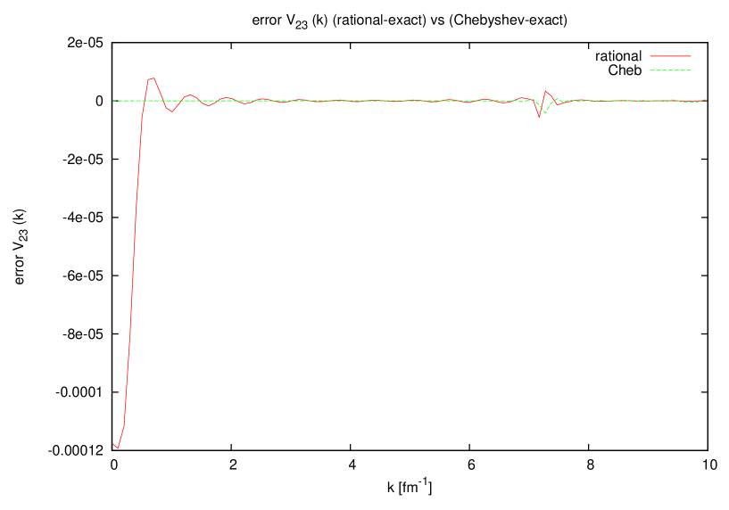
Figure 25: $\Delta V_{13a\,rational}(k),\,\Delta V_{13a\,Chebyshev}(k)$.

References

• (1) R.B. Wiringa, V.G.J. Stoks, R. Schiavilla, Phys. Rev. C51(1995)38.
• (2) V.G.J. Stoks, R.A.M. Klomp, C.P.F. Terheggen, J. J. de Swart, Phys. Rev. C49(1994)2950.
• (3) R. Machleidt, Phys. Rev. C63(2001)024001.
• (4) W. GlΓΆckle, H. Witala, D. HΓΌber, H. Kamada, J. Golak, Phys. Rep. 274Β , 107 (1986).
• (5) S. Veerasamy, University of Iowa Thesis, 2011.
• (6) R. Broucke, Communications of the Association for Computing Machinery, 16,(1973)254.
• (7) B. D. Keister and W. N. Polyzou, J. Comp. Phys. 134(1997),231.
• (8) J. Golak, W. GlΓΆckle , R. SkibiΕ„ski, H. WitaΕ‚a, D. Rozpkedzik, K. Topolnicki, I. Fachruddin, Ch. Elster, A. Nogga, Phys. Rev. C81(2010)034006.
• (9) Private communication with Robert Wiringa.
• (10) http://arxiv.org/abs/arXiv:0911.4173 .
• (11) I. S. Gradshteyn and I. M. Ryzhik, Tables of Integrals, Series, and Products, Associated Press, (1965), page 711 eq. 6.621.
• (12) N. Auerbach, J. HΓΌfner, A. K. Kerman, and C. M. Shakin, Β Reviews of Modern Physics, 44,(1972)48.
• (13) I. S. Gradshteyn and I. M. Ryzhik, Tables of Integrals, Series, and Products, Associated Press, (1965), page 583 eq. 4.381,page 605 eq. 4.401.
Refer to caption