Lyapunov stochastic stability and control of robust dynamic coalitional games with transferable utilities

Abstract

This paper considers a dynamic game with transferable utilities (TU), where the characteristic function is a continuous-time bounded mean ergodic process. A central planner interacts continuously over time with the players by choosing the instantaneous allocations subject to budget constraints. Before the game starts, the central planner knows the nature of the process (bounded mean ergodic), the bounded set from which the coalitions’ values are sampled, and the long run average coalitions’ values. On the other hand, he has no knowledge of the underlying probability function generating the coalitions’ values. Our goal is to find allocation rules that use a measure of the extra reward that a coalition has received up to the current time by re-distributing the budget among the players. The objective is two-fold: i) guaranteeing convergence of the average allocations to the core (or a specific point in the core) of the average game, ii) driving the coalitions’ excesses to an a priori given cone. The resulting allocation rules are robust as they guarantee the aforementioned convergence properties despite the uncertain and time-varying nature of the coaltions’ values. We highlight three main contributions. First, we design an allocation rule based on full observation of the extra reward so that the average allocation approaches a specific point in the core of the average game, while the coalitions’ excesses converge to an a priori given direction. Second, we design a new allocation rule based on partial observation on the extra reward so that the average allocation converges to the core of the average game, while the coalitions’ excesses converge to an a priori given cone. And third, we establish connections to approachability theory [9, 18] and attainability theory [4, 19].

Keywords Coalitional games with transferable utilities; allocation processes; approachability theory; Lyapunov stochastic stability.

I Introduction

Coalitional games with transferable utilities (TU), introduced first by Von Neuman and Morgenstern [25], have recently sparked much interest in the control and communication engineering communities [21]. In essence, coalitional TU games are comprised of a set of players who can form coalitions and a characteristic function associating a real number with every coalition. This real number represents the value of the coalition and can be thought of as a monetary value that can be distributed among the members of the coalition according to some appropriate fairness allocation rule. The value of a coalition also reflects the monetary benefit demanded by a coalition to be a part of the grand coalition.

This paper considers a dynamic TU game, where the characteristic function is a bounded mean ergodic process. Bounded means that the characteristic function takes values in a convex set according to an unknown probability distribution. Mean ergodic means that the expected value of the coalitions values at each time coincides with the long term average. With the dynamic game we associate a dynamic average game obtained by averaging over time the coalitions’ values, and assume that the core of the average game is nonempty on the long run. Given the above dynamic TU game, a central planner interacts continuously over time with the players by choosing the instantaneous allocations subject to budget constraints. Before the game starts, the central planner knows the nature of the process (bounded mean ergodic), the bounded set and the long run average coalitions’ values. On the other hand, he has no knowledge of the underlying probability function generating the instantaneous coalitions’ values. Our goal is to find allocation rules that use a measure of the extra reward that a coalition has received up to the current time by re-distributing the budget among the players. The objective is two-fold: i) guaranteeing convergence of the average allocations to the core (or a specific point in the core) of the average game, ii) driving the coalitions’ excesses to an a priori given cone. The resulting allocation rules are robust as they guarantee the aforementioned convergence properties despite the uncertain and time-varying nature of the coaltions’ values.

In the context of coalitional TU games, robustness and dynamics naturally arise in all the situations where the coalitions values are uncertain and time-varying, see e.g., [7]. Robustness has to do with modeling coalitions’ values as unknown entities and this is in spirit with some literature on stochastic coalitional games [23, 24]. However, we deviate from the latter works since the probability function generating the random coalitions values is unknown, and this is more in line with the concept of Unknown But Bounded (UBB) variables formalized in [8]. It is worth to mention that this formulation shares some common elements with the recent literature on interval valued games [1], where the authors use intervals to describe coalitions values quite similar to what is done in this paper. The interval nature of coalitions’ values arises generally due to the optimistic and pessimistic expectations of the coalitions [11] when cooperation is achieved from a strategic form game. We also note some differences in that we focus here more on the time-varying nature of the coalitions’ values. In doing so, we also link the approach to the set invariance theory [10] and stochastic stability theory [20] which provides us some nice tools for stability analysis (see, e.g., the use of a Lyapunov function in the proof of Theorem IV.1).

Bringing dynamical aspects into the framework of coalitional TU games is an element in common with other papers [13, 16, 17]. The main difference with those works is that the values of coalitions are realized exogenously and no relation exists between consecutive samples.

Convergence conditions together with the idea that allocation rules use a measure of the extra reward that a coalition has received up to the current time by re-distributing the budget among the players are a main issue in a number of other papers [2, 12, 15, 18, 22] as well. However, this paper departs from the aforementioned ones mainly in that dynamics in those works is captured by a bargaining mechanism with fixed coalitions’ values while we let the values be time-varying and uncertain. This last element adds some robustness to our allocation rule which has not been dealt with before.

The main contribution of this paper is captured by the following three results. First, we design an allocation rule based on full observation of the extra reward so that the average allocation approaches a specific point in the core of the average game, while the coalitions’ excesses converge to an a priori given direction. Second, we design a new allocation rule based on partial observation on the extra reward so that the average allocation converges to the core of the average game, while the coalitions’ excesses converge to an a priori given cone. Convergence of both allocation rules is proved via Lyapunov stochastic stability theory. And third, we establish connections of the Lyapunov stochastic stability theory to the approachability theory [9, 18] and attainability theory [4, 19].

A few other contributions of the paper are the definition of average game, whose role becomes fundamental when the coalitions’ values variations are known with delay by the planner; the reformulation of the problem as a network flow control problem, where the allocation rule turns into a robust control policy is a novel aspect, with the importance of such a reformulation lying in the fact that we can prove the convergence of the allocations using the strong tools of the Lyapunov stochastic stability theory; and finally, the idea of turning a coalitional TU game set up into a control theoretic problem is a novel one, which represents, by far, the main characteristics of this work.

The paper is organized as follows. In Section II, we formulate the problem. In Section III, we present the basic idea of our solution approach. In Section IV we state the three main results of this work and postpone the derivation of such results to Section V. In Section VI, we provide some numerical illustrations. Finally, in Section VII, we draw some concluding remarks.

Notation. We view vectors as columns. For a vector $x$, we use $x_{i}$ or $[x]_{i}$ to denote its $i$th coordinate component. For two vectors $x$ and $y$, we use $x<y$ ($x\leq y$) to denote $x_{i}<y_{i}$ ($x_{i}\leq y_{i}$) for all coordinate indices $i$. We let $x^{T}$ denote the transpose of a vector $x$, and $\|x\|_{n}$ denote its $n$-norm. For a matrix $A$, we use $a_{ij}$ or $[A]_{ij}$ to denote its $ij$th entry. We use $|a_{ij}|$ to denote the absolute value of scalar $a_{ij}$. Given two sets $U$ and $S$, we write $U\subset S$ to denote that $U$ is a proper subset of $S$. We use $|S|$ for the cardinality of a given finite set $S$. Let $\Phi$ be a closed and convex set in $\mathbb{R}^{m}$, we use $P(y)$ to denote the projection of any point $y\in\mathbb{R}^{m}$ onto $\Phi$ (closest point to $y$ in $\Phi$). We also denote by $\partial\Phi$ the boundary of $\Phi$ and $n_{y}$ the outward normal for any $y\in\partial\Phi$. We use $dist(y,\Phi)$ to denote the euclidean distance between point $y$ and set $\Phi$. Given a set $N$ of players and a function $\eta:S\mapsto\mathbb{R}$ defined for each nonempty coalition $S\subseteq N$, we write $<N,\eta>$ to denote the transferable utility (TU) game with the players’ set $N$ and the characteristic function $\eta$. We let $\eta_{S}$ be the value $\eta(S)$ of the characteristic function $\eta$ associated with a nonempty coalition $S\subseteq N$. Given a TU game $<N,\eta>$, we use $C(\eta)$ to denote the core of the game, $C(\eta)=\left\{x\in\mathbb{R}^{|N|}\,\Big{|}\,\sum_{i\in N}x_{i}=\eta_{N},\ \sum_{i\in S}x_{i}\geq\eta_{S}\hbox{ for all nonempty }S\subset N\right\}.$ Also, $\mathbb{R}_{+}$ denotes the set of nonnegative real numbers. Given a random vector $\xi$ the notation $\mathbb{E}[\xi]$ denotes its expected value. Given a random process $\{v(t)\}$ we denote by $\tilde{v}(t)=\int_{0}^{t}v(\tau)d\tau$, its integral and $\bar{v}(t)=\frac{\tilde{v}(t)}{t}$ its average up to time $t$.

II Model and problem formulation

In this section, we formulate the problem in its generic form and elaborate on the role of information. Let $N=\{1,\ldots,n\}$ be a set of players and $S\subseteq N$ the set of all (nonempty) coalitions arising among these players. Denote by $m=2^{n}-1$ the number of possible coalitions. We assume that time is continuous and use $t\in\mathbb{R}_{+}$ to index the time slots.

We consider a dynamic TU game, denoted $<N,\{v(t)\}>$, where $\{v(t)\}$ is a continuous flow of characteristic functions. The flow $\{v(t)\}$ describes a bounded mean ergodic process. By bounded we mean that given a bounded convex set $\mathcal{V}\in\mathbb{R}^{m}$ and a probability function $\mathbb{P}\in\Delta(\mathcal{V})$, where $\Delta(\mathcal{V})$ is the set of probability functions on $\mathcal{V}$, then for all $t\in\mathbb{R}_{+}$ each random variable $v(t)$ takes values in $\mathcal{V}\in\mathbb{R}^{m}$ according to probability $\mathbb{P}$ as expressed in (1); by mean ergodic we mean that its expected value coincides with the long term average as in (2):

$$v(t)\in\mathcal{V}\subset\mathbb{R}^{m},\quad\mbox{for all }t\in\mathbb{R}_{+}$$ (1)

$$\mathbb{E}[v(t)]=lim_{\tau\rightarrow\infty}\bar{v}(\tau),\quad\mbox{for all }t\in\mathbb{R}_{+}.$$ (2)

Thus, in the dynamic TU game $<N,\{v(t)\}>$, the players are involved in a sequence of instantaneous TU games whereby, at each time $t$, the instantaneous TU game is $<N,v(t)>$ with $v(t)\in\mathcal{V}$ for all $t\geq 0$. Further, we let $v_{S}(t)$ denote the value assigned to a nonempty coalition $S\subseteq N$ in the instantaneous game $<N,v(t)>$.

With the dynamic game we associate a dynamic average game $<N,\{\bar{v}(t)\}>$ and an instantaneous average game at time $t\geq 0$, $<N,\bar{v}(t)>$.

The motivation of formalizing the above dynamic TU games is in that such games represent a stylized model of all those scenarios where the coalitions’ values vary with time.

We assume that the core of the average game is nonempty on the long run. We will see that without this assumption the problem under study has no solution. Thus, denote by $v_{nom}$ the (long run) average coalitions’ values, namely, $v_{nom}:=\lim_{t\rightarrow\infty}\bar{v}(t)$ and let $C(v_{nom})$ be the core of the average game.

Assumption 1

(balancedness) The core of the average game is nonempty in the limit: $C(v_{nom})\not=\emptyset$.

We can view the above assumption as introducing some steady-state (average) conditions on a game scenario subject to instantaneous fluctuations. However, note that we do not make assumptions regarding the balancedness of the instantaneous games which is the case with [7]. Thus, the core of the instantaneous game can be empty at some time $t$.

Given the above dynamic TU game, a central planner interacts continuously over time with the players by choosing the instantaneous allocations denoted by $a(t)\in\mathbb{R}^{n}$. We assume that the allocations are subject to the following budget constraints.

Assumption 2

(bounded allocation) The instantaneous allocation is bounded within a hyperbox in $\mathbb{R}^{n}$

$$a(t)\in\mathcal{A}:=\{a\in\mathbb{R}^{n}:\,a_{min}\leq a\leq a_{max}\},$$

with a priori given lower and upper bounds $a_{min}$, $a_{max}\in\mathbb{R}^{n}$.

As regards the information available a priori (before the game starts) to the central planner, we assume that he knows the nature of the process $\{v(t))\}$ (bounded mean ergodic), the bounded set $\mathcal{V}$ and the long run average coalitions’ values $v_{nom}$. The latter is the same as saying that he knows the expected coalitions’ values for all $t\in\mathbb{R}_{+}$. On the other hand, he has no knowledge of the underlying probability function $\mathbb{P}$.

Assumption 3

(on available information) The planner knows $v_{nom}$.

Beside this, during the game the central planner also observes the extra reward of the coalitions up to $t$ and for all $t\in\mathbb{R}_{+}$. Given this, and in line with a number of other papers [2, 12, 15, 18, 22], our goal is to find allocation rules that use a measure of the extra reward that a coalition has received up to the current time by re-distributing the budget among the players. To do this, a first step is to define excesses for the coalitions. For any coalition $S\subseteq N$, we define excess (extra reward) at time $t\geq 0$ as the excess at time $t=0$ plus the difference between the total integral reward, given to it, and the integral value of the coalition itself, i.e.,

$${\epsilon}_{S}(t)=\sum_{i\in S}\tilde{a}_{i}(t)-\tilde{v}_{S}(t)+{\epsilon}_{S}(0).$$

Furthermore, assuming without loss of generality ${\epsilon}_{S}(0)=0$, we say that $S$ is in excess at time $t\geq 0$ if the excess is nonnegative, i.e., $\sum_{i\in S}\tilde{a}_{i}(t)\geq\tilde{v}_{S}(t)$. Let $\epsilon(t)$ represent the vector of coalitions’ excesses, formally given as:

$$\epsilon(t)=\left\{\epsilon_{S}(t)\right\}_{N\supseteq S\neq\emptyset}.$$

We are interested in answering two main questions for this class of games.

• Question 1: Are there allocation rules such that the average allocations converge? If yes, let us denote by $\mathcal{A}_{0}$ the set where the average allocations converge to. Can we make it converge to the core of the average game $\mathcal{A}_{0}\subseteq C(v_{nom})$? Can we guarantee the convergence to a specific point of the core, call it nominal allocation $a_{nom}$, that we have a priori selected?

• Question 2: Are there allocation rules such that the coalitions’ excesses $\epsilon(t)$ converge to an a priori given cone $\Sigma_{0}$, say for instance the nonnegative $m$-dimensional orthant $\mathbb{R}_{+}^{m}$, or any direction $\alpha t$ for $t\geq 0$ with fixed $\alpha\in\mathbb{R}_{+}^{m}$?

To motivate the above questions think of a situation where the objective of the central planner is to maintain the stability of grand coalition in an average sense, while controlling the coalitions’ excesses at each time $t\in\mathbb{R}_{+}$.

We are now in the position of providing a formal and generic statement of the problem. Henceforth, we use the symbol w.p.1 to mean “with probability one”.

Problem II.1

Find an allocation rule $f:\mathbb{R}^{m}\rightarrow\mathcal{A}\in\mathbb{R}^{n}$, such that if $a(t)=f\left(\epsilon(t)\right)$ then i) $\lim_{t\rightarrow\infty}\bar{a}(t)\in\mathcal{A}_{0}\subseteq C(v_{nom})$ w.p.1, and ii) $\lim_{t\rightarrow\infty}\epsilon(t)\in\Sigma_{0}\subseteq\mathbb{R}_{+}^{m}$ w.p.1.

Observe that because of the random nature of the coalitions’ values $v(t)$, both the excesses $\epsilon(t)$ and the allocations $a(t)$ are random and as such we look at the convergence of $\bar{a}(t)$ w.p.1. Essentially, we require that the probability of $\bar{a}(t)$ converging in the limit to $\mathcal{A}_{0}\subseteq C(v_{nom})$ is 1. Similarly for $\epsilon(t)$ and $\Sigma_{0}$. This type of convergence is also known as almost sure convergence [20].

We will show that if the planner has full observation of $\epsilon(t)$ at every time $t$ then the above problem is solvable even under the very strict condition of $\mathcal{A}_{0}=a_{nom}$ and $\Sigma_{0}=\alpha t$ $t\geq 0$ with fixed $\alpha$. Conversely, if the planner has partial observation of $\epsilon(t)$ in that he only knows the sign of each component of $\epsilon(t)$, then the problem is still solvable but under the relaxed condition of $\mathcal{A}_{0}=C(v_{nom})$ and $\Sigma_{0}\subseteq\mathbb{R}_{+}^{m}$.

II-A Motivations

Dynamic coalitional games capture coordination in a number of network flow applications. Network flows model flow of goods, materials, or other resources between different production/distribution sites [3]. We next provide a supply chain application that justifies the model under study.

A single warehouse ${\bf v}_{0}$ serves a number of retailers ${\bf v}_{i}$, $i=1,\ldots,n$, each one facing a demand $d_{i}(t)$ unknown but bounded by pre-assigned values $d_{i}^{\min}\in\mathbb{R}$ and $d_{i}^{\max}\in\mathbb{R}$ at any time period $t\geq 0$. After demand $d_{i}(t)$ has been realized, retailer ${\bf v}_{i}$ must choose to either fulfill the demand or not. The retailers do not hold any private inventory and, therefore, if they wish to fulfill their demands, they must reorder goods from the central warehouse. Retailers benefit from joint reorders as they may share the total transportation cost $K$ (this cost could also be time and/or players dependent). In particular, if retailer ${\bf v}_{i}$ “plays” individually, the cost of reordering coincides with the full transportation cost $K$. Actually, when necessary a single truck will serve only him and get back to the warehouse. This is illustrated by the dashed cycles $({\bf v}_{0},{\bf v}_{8},{\bf v}_{0})$, $({\bf v}_{0},{\bf v}_{9},{\bf v}_{0})$, and $({\bf v}_{0},{\bf v}_{10},{\bf v}_{0})$ in the network of Figure 1. The cost of not reordering is the cost of the unfulfilled demand $d_{i}(t)$.

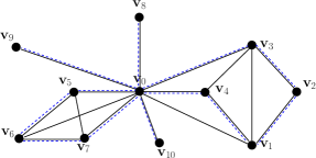
(a) Five trucks (cycles) leaving ${\bf v}_{0}$ and serving coalitions $\{{\bf v}_{1},\ldots,{\bf v}_{4}\}$, $\{{\bf v}_{5},\ldots,{\bf v}_{7}\}$, $\{{\bf v}_{8}\}$, $\{{\bf v}_{9}\}$, and $\{{\bf v}_{10}\}$ respectively.

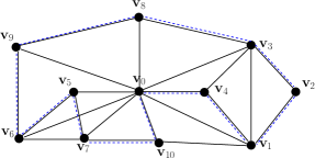
(b) One single truck (cycle) leaving ${\bf v}_{0}$ and serving coalition $\{{\bf v}_{1},\ldots,{\bf v}_{10}\}$.

Figure 1: Example of a distribution network

If two or more retailers “play” in a coalition, they agree on a joint decision (“everyone reorders” or “no one reorders”). The cost of reordering for the coalition also equals the total transportation cost that must be shared among the retailers. In this case, when necessary a single truck will serve all retailers in the coalition and get back to the warehouse. This is illustrated, with reference to coalition $\{{\bf v}_{1},\ldots,{\bf v}_{4}\}$ by the dashed cycle $({\bf v}_{0},{\bf v}_{4},{\bf v}_{1},{\bf v}_{2},{\bf v}_{3},{\bf v}_{0})$ in Figure 1(a). A similar comment applies to the coalition $\{{\bf v}_{5},{\bf v}_{6},{\bf v}_{7}\}$ and the cycle $({\bf v}_{0},{\bf v}_{5},{\bf v}_{6},{\bf v}_{7},{\bf v}_{0})$ in Figure 1(a). The network topology in Figure 1(a) describes the existing coalitions. This is clear if we look at the subgraph induced by the vertex-set $\{{\bf v}_{1},\ldots,{\bf v}_{10}\}$ (all vertices except ${\bf v}_{0}$) and observe that such a subgraph has 5 connected components, i.e., $\{{\bf v}_{1},\ldots,{\bf v}_{4}\}$, $\{{\bf v}_{5},\ldots,{\bf v}_{7}\}$, $\{{\bf v}_{8}\}$, $\{{\bf v}_{9}\}$, and $\{{\bf v}_{10}\}$ and that each component corresponds to an existing coalition. The cost of not reordering is the sum of the unfulfilled demands of all retailers. How the players will share the cost is a part of the solution generated by the bargaining process.

Conversely, the subgraph induced by $\{{\bf v}_{1},\ldots,{\bf v}_{10}\}$ in Figure 1(b) has a single connected component which means that all retailers “play” in the grand coalition and as such one single truck (cycle) will leave ${\bf v}_{0}$ and serve all of them before returning to ${\bf v}_{0}$. This is represented by the dashed cycle $({\bf v}_{0},{\bf v}_{4},\ldots,{\bf v}_{10})$ in the same figure.

The cost scheme can be captured by a game with the set $N=\{{\bf v}_{1},\ldots,{\bf v}_{n}\}$ of players where the cost of a nonempty coalition $S\subseteq N$ is given by

$$c_{S}(t)=\min\left\{K,\sum_{i\in S}d_{i}(t)\right\}.$$

Note that the bounds on the demand $d_{i}(t)$ reflect into the bounds on the cost as follows: for all nonempty $S\subseteq N$ and $t\geq 0$,

$$\min\left\{\sum_{i\in S}K,d_{i}^{\min}\right\}\leq c_{S}(t)\leq\min\left\{K,\sum_{i\in S}d_{i}^{\max}\right\}.$$ (3)

To complete the derivation of the coalitions’ values we need to compute the cost savings $v_{S}(t)$ of a coalition $S$ as the difference between the sum of the costs of the coalitions of the individual players in $S$ and the cost of the coalition itself, namely,

$$v_{S}(t)=\sum_{i\in S}c_{\{i\}}(t)-c_{S}(t).$$

Given the bound for $c_{S}(t)$ in (3), the value $v_{S}(t)$ is also bounded, as given: for any $S\subset N$ and $t\geq 0$,

$$v_{S}(t)\leq\sum_{i\in S}\min\left\{K,d_{i}^{\max}\right\}-\min\left\{K,\sum_{i\in S}d_{i}^{\min}\right\}.$$

Thus, the cost savings (value) of each coalition is bounded uniformly by a maximum value.

Introducing time aspects into a static TU game opens the possibility for modeling aspects such as intertemporal transfers, patience and expectations of players/coalitions. A generic dynamic coalitional game description should capture these features. In a repeated joint replenishment game as the one discussed above, allocation rules having the properties formalized in Problem II.1, encourage patient retailers to “play” in the grand coalition, to coordinate their replenishment policies and therefore to reduce total transportation costs. We say patient retailers since condition i) in Problem II.1 guarantees convergence to core on the long-run, i.e., in an average sense. Condition ii) has the meaning of bounding the excesses during the transient (before convergence occurs).

III Flow transformation based dynamics

The basic idea of our solution approach is to recast the problem into a flow control one. To do this, consider the hyper-graph $\mathcal{H}$ with vertex set $V$ and edge set $E$ as:

$$\mathcal{H}:=\{V,E\},\quad V=\{{\bf v}_{1},\ldots,{\bf v}_{m}\},\quad E:=\{{\bf e}_{1},\ldots,{\bf e}_{n}\}.$$

Figure 2 depicts an example of hypergraph for a 3-player coalitional game. The vertex set $V$ has one vertex per each coalition whereas the edge set $E$ has one edge per each player.

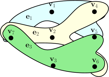
Figure 2: Hypergraph $\mathcal{H}:=\{V,E\}$ for a $3$-player coalitional game.

A generic edge $i$ is incident to a vertex ${\bf v}_{j}$ if the player $i$ is in the coalition associated to ${\bf v}_{j}$. So, incidence relations are described by matrix $B_{\mathcal{H}}$whose rows are the characteristic vectors $c^{S}\in\mathbb{R}^{n}$. We recall that the components of a characteristic vector $c^{S}_{i}=1$ if $i\in S$ and $c^{S}_{i}=0$ if $i\notin S$. The flow control reformulation arises naturally if we view allocation $a_{i}(t)$ as the flow on edge ${\bf e}_{i}$ and the coalition value $v_{S}(t)$ of a generic coalition $S$ as the demand in the corresponding vertex ${\bf v}_{j}$. In view of this, allocation in the core translates into over-satisfying the demand at the vertices. Specifically,

$$a(t)\in C(v(t))\quad\Leftrightarrow\quad B_{\mathcal{H}}a(t)\geq v(t),$$ (4)

with the last inequality satisfied with the equal sign due to the efficiency condition of the core, i.e, $\sum_{i=1}a_{i}(t)=v_{m}(t)$, where $v_{m}(t)$ denotes the $m$th component of $v(t)$ and is equal to the grand coalition value $v_{N}(t)$. Now, since $v(t)$ is unobservable by the planner at time $t$, we need to introduce some allocation error dynamics which accounts for the derivatives of the excesses. Since $\epsilon(t)$ represents the coalition excess, we have:

$$\dot{\epsilon}(t)=B_{\mathcal{H}}a(t)-v(t),\quad v(t)\in\mathcal{V}.$$ (5)

Note that the above differential equation admits a solution at least in the sense of Filippov [14]. From (4) and by averaging and taking the limit in (5), we can reformulate Problem II.1 as a flow control problem where a controller wishes to drive the quantity $\lim_{t\rightarrow\infty}\frac{\epsilon(t)-\epsilon(0)}{t}$ to the target set $\mathcal{T}$, defined below, w.p.1 (see, e.g., Fig. 3):

$$\mathcal{T}:=\{\tau\in\mathbb{R}^{m}:\,\tau_{m}=0,\tau_{j}\geq 0,\,\forall j=1,\ldots,m-1\}.$$

Note, $\tau_{m}=0$ due to efficiency of allocations.

Figure 3: Trajectory for $\frac{\epsilon(t)-\epsilon(0)}{t}$.

Remark III.1

Driving the average allocations to a particular point $a_{nom}\in\mathcal{A}_{0}\subseteq C(v_{nom})$ results in reaching a specific point in the target set $\mathcal{T}$. To see this, note that when $\lim_{t\rightarrow\infty}\bar{a}(t)=a_{nom}$ we have $\mathcal{T}\ni B_{\mathcal{H}}a_{nom}-v_{nom}\geq 0$ due to the property of the core. Thus, we also have that $\lim_{t\rightarrow\infty}\frac{\epsilon(t)-\epsilon(0)}{t}$ is driven to the point $B_{\mathcal{H}}a_{nom}-v_{nom}\in\mathcal{T}$.

The inequality condition in (4) is transformed into equality type by introducing, from standard LP techniques, $m-1$ surplus variables (one per each coalition other than the grand coalition). This increases the dimension of the control space of the planner from $m$ to $n+m-1$ and the dynamics (5) can be rewritten as follows:

$$\dot{x}(t)=Bu(t)-v(t),~{}v(t)\in\mathcal{V}$$ (6)

where $B=\left[B_{\mathcal{H}}~{}\Bigl{|}\begin{array}[]{c}-I_{m-1}\\ 0\end{array}\right]\in\mathbb{R}^{m\times n+m-1}$. Variable $x(t)$ represents the state of the system and captures deviation from the balanced system, i.e., the system characterized by $a_{nom}$ and $v_{nom}$. We introduce the set of feasible controls as:

$$U:=\left\{u(t)\in\mathbb{R}^{n+m-1}:u(t)=[a^{T}(t)~{}~{}s^{T}(t)]^{T},~{}a(t)\in\mathcal{A},~{}s(t)\geq 0\right\}.$$ (7)

Toward the reformulation of the problem as a stochastic stabilizability one, we introduce the following preliminary result.

Lemma III.1

If the variable $x(t)$ is asymptotically stable almost surely, i.e., (8) holds true, then the average allocations converge to the core of the average game w.p.1. as expressed by (9), and the excesses converge to the cone $\mathbb{R}_{+}^{m}$ w.p.1. as described in (10):

$$\lim_{t\rightarrow\infty}{x}(t)=0,\quad\mbox{w.p.1.}$$ (8)

$$\lim_{t\rightarrow\infty}\bar{a}(t)\in C(v_{nom}),\,\mbox{w.p.1}$$ (9)

$$\lim_{t\rightarrow\infty}\epsilon(t)\in\mathbb{R}_{+}^{m},\,\mbox{w.p.1}.$$ (10)

Proof:

To see why (8) implies (9), observe that if $\lim_{t\rightarrow\infty}{x}(t)=0$ w.p.1. then $\lim_{t\rightarrow\infty}\frac{x(t)-x(0)}{t}=0$ w.p.1. and therefore, by integrating and dividing by $t$ in (6) also $\lim_{t\rightarrow\infty}B\bar{u}(t)-\bar{v}(t)=0$ w.p.1. The latter can be rewritten as $\lim_{t\rightarrow\infty}B\bar{u}(t)=v_{nom}$ w.p.1, and as from (7) $\bar{s}(t)=B_{\mathcal{H}}\bar{a}(t)-\bar{v}(t)\geq 0$ and $v_{nom}$ is balanced by Assumption 2 then we conclude that $\lim_{t\rightarrow\infty}\bar{a}(t)\in C(v_{nom})$ w.p.1.

To see why (8) implies (10), observe that if $\lim_{t\rightarrow\infty}{x}(t)=0$ w.p.1., from (7) and under the assumption $x(0)=\epsilon(0)=0$, then $\lim_{t\rightarrow\infty}\epsilon(t)=\lim_{t\rightarrow\infty}\tilde{s}(t)\geq 0$ and (10) is proved.  $\square$

It is worth noting that condition (9) is part of Problem II.1. In other words when solving Problem II.1 we always guarantee (9). If this is clear then, we can use the above lemma to rephrase Problem II.1. In doing this we need to make a partial distinction between cases i) and ii). More specifically, case ii) where $\mathcal{A}_{0}=C(v_{nom})$ can be restated as follows:

$$\text{Find }u(t):=\phi(x(t))\in U\text{ such that }\lim_{t\rightarrow\infty}{x}(t)=0\text{ w.p.1.}$$ (11)

Note that if we wish to reach a specific point $a_{nom}$ then the condition (9) is only necessary and the resulting problem is a stricter version of (11).

IV Main results

In this section we present the three main results of this work. The first one relates to the case where the planner has full observation on $x(t)$ in which case the average allocation can be driven to a specific point in the Core of the average game. The second result applies to the case where the planner has partial observation on $x(t)$, and convergence to the Core can still be guaranteed but not to a specific point of the Core. The third result highlights connections of the implemented solution approach to the approachability principle [9, 18] and attainability principle [4, 19].

IV-A Full information case

In this section, we solve Problem II.1 with $\mathcal{A}_{0}=a_{nom}$ and $\Sigma_{0}=\alpha t,t\geq 0$ with fixed $\alpha$ under the assumption that the planner has full observation of the excesses $\epsilon(t)$ and therefore $x(t)$ as well. We recall that inferring $x(t)$ from $\epsilon(t)$ is possible as the surplus $s(t)$ is selected by the planner. As we have said before, the problem that we solve is a stricter version of (11). This version derives from augmenting the state of dynamics (6) as explained in the rest of this section. Before introducing the augmentation technique let us assume that the fluctuations of the coalitions’ values around the mean $v_{nom}$ are independent of the state $x(t)$. We formalize this in the next assumption where we denote by $\Delta v(t)=v(t)-v_{nom}$ the above fluctuations.

Assumption 4

The state $x(t)$ and the coalitions’ values fluctuations $\Delta v(t)$ are independent.

Introducing the fluctuations $\Delta v(t)$ allows us to rewrite dynamics (6) in a more convenient way. To do this, note first that, as $u(t)=[a(t)^{T}~{}s(t)^{T}]^{T}$ and from $Bu_{nom}=v_{nom}$, if $a_{nom}$ is fixed then $s_{nom}\in\mathbb{R}_{+}^{m-1}$ and therefore also $u_{nom}=[a_{nom}^{T}\>s_{nom}^{T}]^{T}$ are fixed. Let us denote $\Delta u(t)=u(t)-u_{nom}$. Dynamics (6) can be rewritten as follows:

$$\dot{x}(t)=Bu(t)-v(t) = Bu(t)-(v_{nom}+(v(t)-v_{nom}))=Bu(t)-v_{nom}-\Delta v(t)$$

$$= B\left(u(t)-u_{nom}\right)-\Delta v(t)=B\Delta u(t)-\Delta v(t)$$

We mentioned before that we will focus on a stricter version of (11). We do this by augmenting the state as shown next. First, denote by $B^{\dagger}$ a generic pseudo inverse matrix of $B$ and complete matrices $B$ and $B^{\dagger}$ with matrices $C$ and $F$ such that

$$\left[\begin{array}[]{c}B\\ C\end{array}\right]~{}\left[\begin{array}[]{cc}B^{\dagger}&F\end{array}\right]=I.$$ (12)

Then, building upon the new square matrix $\left[\begin{array}[]{c}B\\ C\end{array}\right]$, let us consider the augmented system

$$\begin{array}[]{rcl}\dot{x}(t)&=&B\Delta u(t)-\Delta v(t)\\ \dot{y}(t)&=&C\Delta u(t).\end{array}$$ (13)

Here we assume that $v(t)$ is independent of $y(t)$ as well. After integrating the above system (see (14), right) we define a new variable $z(t)$ as follows:

$$z(t)=\left[\begin{array}[]{cc}B^{\dagger}&F\end{array}\right]~{}\left[\begin{array}[]{c}x(t)\\ y(t)\end{array}\right],~{}~{}~{}\left[\begin{array}[]{c}x(t)\\ y(t)\end{array}\right]=\left[\begin{array}[]{c}B\\ C\end{array}\right]~{}z(t).$$ (14)

It turns out that to drive $x(t)$ to zero w.p.1, and obtain $u_{nom}$ as average allocation on the long run, we can rely on a simple function $\hat{\phi}(.)$, which depends on $z(t)$. Before introducing this function, for future purposes observe that the dynamics for $z(t)$ satisfies the first-order differential equation:

Figure 4: Dynamical System

$$\begin{array}[]{lll}\dot{z}(t)&=&\left[\begin{array}[]{cc}B^{\dagger}&F\end{array}\right]~{}\left[\begin{array}[]{c}\dot{x}(t)\\ \dot{y}(t)\end{array}\right]\\ &=&\left[\begin{array}[]{cc}B^{\dagger}&F\end{array}\right]~{}\left[\begin{array}[]{c}B\\ C\end{array}\right]\Delta u(t)-\left[\begin{array}[]{cc}B^{\dagger}&F\end{array}\right]\left[\begin{array}[]{c}\Delta v(t)\\ 0\end{array}\right]\\ &=&\Delta u(t)-B^{\dagger}\Delta v(t).\end{array}$$ (15)

Let $\Delta u^{min}$ and $\Delta u^{max}$ be the minimal and maximal values of $\Delta u(t)$ for the following constraints to hold true: $u(t)=u_{nom}+\Delta u(t)\in U$. Then, let us formally define $\hat{\phi}(z(t))$ as:

$$\hat{\phi}(z(t)):=u_{nom}+\Delta u(t)\in U,\quad\Delta u(t)=sat_{[\Delta u^{min},~{}\Delta u^{max}]}(-z(t)),$$ (16)

where with $sat_{[a,b]}(\xi)$ we denote the saturated function that, given a generic vector $\xi$ and lower and upper bounds $a$ and $b$ of same dimensions as $\xi$, returns

$$sat_{[a,b]}(\xi)\doteq\left\{\begin{array}[]{lll}b_{i}&\mbox{for all $i$}&\xi_{i}>b_{i}\\ a_{i}&\mbox{for all $i$}&\xi_{i}<a_{i}\\ \xi_{i}&\mbox{for all $i$}&a_{i}\leq\xi_{i}\leq b_{i}\end{array}\right..$$

Now, taking the control $u(t)=\hat{\phi}(z(t))$, we obtain the dynamic system $\dot{z}(t)=B\hat{\phi}(z(t))-v(t)$ as displayed in Fig. 4. With the above preamble in mind, we are ready to state the following convergence property.

Theorem IV.1

Using the controller $\hat{\phi}(z(t))$, as in (16), we have $\lim_{t\rightarrow\infty}z(t)=0$ w.p.1 and therefore $\lim_{t\rightarrow\infty}\bar{u}(t)=u_{nom}$.

In the next corollary, we use the previous result to provide an answer to Problem II.1.

Corollary IV.1

The state $x(t)$ is driven to zero w.p.1 as expressed in (11), the average allocation converges to the nominal allocation i.e., $\lim_{t\rightarrow\infty}\bar{a}(t)=a_{nom}$, w.p.1 and the excesses converge to the direction $\Sigma_{0}=\alpha t$ with $\alpha=s_{nom}$, i.e., $\lim_{t\rightarrow\infty}\epsilon(t)\in\Sigma_{0}$.

Proof:

This is a direct consequence of the result proved in the previous theorem. From (14), and $[B^{\dagger}~{}F]$ being a non singular matrix, we have $\lim_{t\rightarrow\infty}x(t)=0$ w.p.1. From the previous theorem we also have $\lim_{t\rightarrow\infty}\bar{u}(t)=u_{nom}$. Since $u(t)=[a^{T}(t)~{}s^{T}(t)]^{T}$, we have that $\lim_{t\rightarrow\infty}\bar{a}(t)=a_{nom}$ and $\lim_{t\rightarrow\infty}\epsilon(t)=\tilde{s}(t)=s_{nom}t$.  $\square$

To summarize, in the full information case, the controller $u(t)$ defined by (16) induces an allocation sequence $a(t)$ such that the average $\bar{a}(t)$ converges to $\mathcal{A}_{0}=a_{nom}$ and the excesses approach $s_{nom}t$.

IV-B Partial information case

In the previous section we observed that if the planner has full observation of the excesses and therefore of $x(t)$ then he can design an allocation rule so that the average allocations are driven to $a_{nom}$ and the excesses approach $s_{nom}t$. In this section, we solve Problem II.1 with $\mathcal{A}_{0}=C(v_{nom})$ and under the assumption that the planner has partial observation of $x(t)$. In particular, we assume that the planner observes the sign of $x(t)$ for all $t\in\mathbb{R}_{+}$. An information structure based on the sign of $x(t)$ has an oracle-based interpretation which we discuss in detail in Subsection IV-B1.

Similarly to the previous section, suppose that we know a particular allocation $a_{nom}$ in the core $C(v_{nom})$, and let us study the convergence properties of the average allocations. In particular, using an allocation rule $u(t)=\phi(x(t))$, we require that $x(t)$ satisfying the dynamics $\dot{x}(t)=B\phi(x(t))-v(t)$, converge to zero in probability. In this section, we state the second main result of this work which provides a solution to Problem II.1 with partial information structure. To do this, let us denote again by $B^{\dagger}$ a generic pseudo inverse matrix of $B$ and take a feasible allocation $u_{nom}$ such that

$$Bu_{nom}=v_{nom}:=\lim_{t\rightarrow\infty}\bar{v}(t),\quad u_{nom}\in U.$$

Also, for future purposes, define a function $\hat{\phi}(.)$, which depends only on the sign of $x(t)$, as follows:

$$\hat{\phi}(sgn(x(t))):=u_{nom}+\Delta u(t)\in U,\quad\Delta u(t)=-\delta B^{\dagger}sgn(x(t)).$$ (17)

Now, taking the control $u(t)=\hat{\phi}(sgn(x(t)))$, we obtain the dynamic system $\dot{x}(t)=B\hat{\phi}(sgn(x(t)))-v(t)$ as displayed in Fig. 5. Now, we state the following convergence property.

Figure 5: Dynamical System

Theorem IV.2

Using the controller $u(t)=\hat{\phi}(sgn(x(t)))$ as in (17) we have $\lim_{t\rightarrow\infty}x(t)=0$ w.p.1.

Corollary IV.2

The average allocation converges to the core of the average game as in (9) and the excesses $\epsilon(t)$ converge to $\mathbb{R}_{+}^{m}$ as in (10).

Proof:

Direct consequence of Theorem IV.2 and Lemma III.1.  $\square$

IV-B1 Oracle-based interpretation

In this subsection we elaborate more on the partial information structure. In particular, we highlight how the feedback on state $x(t)$ can be reviewed as the result of an oracle-based procedure. To see this, assume that the planner knows the sign of $x(t)$. Since $x(t)=\left(\epsilon(t)-\tilde{s}(t)\right)-\left(\epsilon(0)-x(0)\right)$, $\text{sgn}(x(t))$ reflects over-satisfaction of coalitions with respect to the threshold $\tilde{s}(t)$. In particular, take without loss of generality $\epsilon(0),x(0)=0$, then with reference to component $j$, the sign of $x_{j}(t)$ yields:

$$sgn\left(x_{j}(t)\right):=\left\{\begin{array}[]{cl}1&\epsilon_{j}(t)>\tilde{s}_{j}(t)\\ 0&\epsilon_{j}(t)=\tilde{s}_{j}(t)\\ -1&\epsilon_{j}(t)<\tilde{s}_{j}(t).\end{array}\right.$$ (18)

To summarize, we can think of a situation where the planner approaches an oracle that tells him the sign of $x(t)$. Since $s(t)$ is chosen by the planner for every $t$, the accumulated surplus, $\tilde{s}(t)$, is given as an input to the oracle. The oracle returns “yes” if the actual excess is greater than $\tilde{s}(t)$ and “no” otherwise. The use of an oracle is an element in common with the ellipsoid method in optimization and with a large literature [26] on cutting planes.

Recall that nonnegativeness of the threshold has its roots in the feasibility condition $u(t)\in U$ for all $t\geq 0$ with feasible set $U$ as in (7).

Nonnegativeness of the threshold provides us with a further comment on the information available to the planner. Actually, from the first condition in (18), we can conclude that coalitions associated to a positive state $x(t)$ are certainly in excess. This is clear if we observe that $sgn\left(x_{j}(t)\right)=1$ implies $\epsilon_{j}(t)>\tilde{s}_{j}(t)\geq 0$. We can then summarize the information content available to the planner as follows, where $S$ is the generic coalition associated with component $j$:

$$sgn\left(x_{j}(t)\right):=\left\{\begin{array}[]{cl}1&\mbox{then coalition $S$ in excess}\\ -1,0&\mbox{nothing can be said}.\end{array}\right.$$

Trivially, the development in the full information case in Section IV-A, which is all based on control strategy (16), fits the case where $x(t)$ is revealed completely. In this last case, the fact that the planner knows $x(t)$ implies that he knows $\epsilon(t)$ as well. Also, it is intuitive to infer that in this last set up, exact knowledge of $x(t)$ can only influence positively the planner in terms of speed of convergence of allocations to the core of the average game.

Remark IV.1

As the planner knows a priori the nominal game and a corresponding nominal allocation vector, a natural question that arises is why one has to design an allocation rule as given by (16) and (17) instead of a stationary rule $\hat{\phi}(.)=u_{nom}$. The rules given by (16) and (17) intuitively translate to meeting the demands of coalitions in an average sense. This feature reflects patience aspect of coalitions in a dynamic setting, i.e., even if a demand is not met instantaneously a coalition is willing to wait and stay in the grand coalition as the demand is fulfilled in an average sense.

IV-C Connections to Approachability and Attainability

IV-C1 Approachability

Approachability theory was developed by Blackwell in 1956 [9] and is captured in the well known Blackwell’s Theorem. Along the lines of Section 3.2 in [18], we recall next the geometric (approachability) principle that lies behind Blackwell’s Theorem. The goal of this section is to show that such a geometric principle shares striking similarities with the solution approach used in the previous sections.

To introduce the approachability principle, let $\Phi$ be a closed and convex set in $\mathbb{R}^{m}$ and let $P(y)$ be the projection of any point $y\in\mathbb{R}^{m}$ (closest point to $y$ in $\Phi$). Also denote by $\bar{y}_{k}$ the average of $y_{1}\ldots,y_{k}$, i.e., $\bar{y}_{k}=\frac{\sum_{t=0}^{k}y_{t}}{k}$ and let $dist(\bar{y}_{k},\Phi)$ be the euclidean distance between point $\bar{y}_{k}$ and set $\Phi$.

Lemma IV.1

(Approachability principle [18]) Suppose that a sequence of uniformly bounded vectors $y_{k}$ in $\mathbb{R}^{m}$ satisfies condition (19),

$$[\bar{y}_{k}-P(\bar{y}_{k})]^{T}[y_{k+1}-P(\bar{y}_{k})]\leq 0,$$ (19)

then $\lim_{k\rightarrow\infty}dist(\bar{y}_{k},\Phi)=0$.

Now, to make use of the above principle in our set up, let us consider the discrete time analog of the excess dynamics (6):

$$x_{k+1}=x_{k}+B\Delta u_{k}-\Delta v_{k},$$

and define a new variable $y_{k}=x_{k}-x_{k-1}$ so that we can look at the sequence of $y_{k}$ in $\mathbb{R}^{m}$. Likewise, consider the discrete time version of control (17) as displayed below:

$$\hat{\phi}(sgn(x_{k})):=u_{nom}+\Delta u_{k}\in U,\quad\Delta u_{k}=-\delta B^{\dagger}sgn(x_{k}-x_{0}).$$ (20)

We are now in a position to state the main result of this section.

Theorem IV.3

Using the controller $u_{k}=\hat{\phi}(sgn(x_{k}-x_{0}))$ as in (20) we have that

• the vector $0$ is approachable by the sequence $\bar{y}_{k}$,

  $$\lim_{k\rightarrow\infty}\bar{y}_{k}=0,\,\mbox{w.p.1},$$ (21)

  and therefore

• the average allocations converge to the core of the average game,

  $$\lim_{k\rightarrow\infty}\bar{a}_{k}\in C(v_{nom}),\,\mbox{w.p.1}.$$ (22)

The strength of the above result is in that it sheds light on how the convergence problem dealt with in this work has a stochastic stability interpretation as well as an approachability one.

Remark IV.2

(Continuous-time approachability) We can reformulate Theorem IV.3 in the continuous time. To see this, let us first define $y(t):=\dot{x}(t)$. Next we need to derive the continuous time version of (19). To this aim, let $t\rightarrow r(t)$ be a differentiable continuous time variable and let $z(t)=\frac{r(t)-r(0)}{t}$, so $t\dot{z}(t)+z(t)=\dot{r}(t)$. Discrete time versions are given as $z_{k}=\frac{1}{k}r_{k}$ and $z_{k+1}=\frac{1}{k+1}r_{k+1}$. The approachability principle is given as

$$\left[z_{k}-P(z_{k})\right]^{T}\left[\phi-P(z_{k})\right]\leq 0$$

where $\phi=(k+1)z_{k+1}-kz_{k}$. In continuous time the above condition translates to

$$\left[z(t)-P(z(t))\right]^{T}\left[\phi-P(z(t))\right]\leq 0$$

and $\phi=(t+\Delta t)z(t+\Delta t)-tz(t)=t\left(z(t+\Delta t)-z(t)\right)+\Delta tz(t+\Delta t)$. We see that $\frac{\phi}{\Delta t}=t\frac{z(t+\Delta t)-z(t)}{\Delta t}+z(t+\Delta t)$. Further, as $\Delta t\rightarrow 0$ we have $\lim_{\Delta t\rightarrow 0}\frac{\phi}{\Delta t}=t\dot{z}(t)+z(t)=\dot{r}(t)$. The approachability principle in continuous time can then be reproposed as

$$\left[z(t)-P(z(t))\right]^{T}\left[\dot{r}(t)-P(z(t))\right]\leq 0,$$ (23)

which constitutes the continuous time version of (19). If $\Phi=\{0\}$ we have $P(z(t))=0$ and $z^{T}(t)\dot{r}(t)\leq 0$. Now, taking $r(t)=x(t)$ we see that $z(t)$ is the average of $y(t)$. Then condition (23) guarantees that $z(t)$ converges to zero as well as $\bar{y}(t)$. But this implies that $\lim_{t\rightarrow\infty}\frac{x(t)-x(0)}{t}=0$ and therefore from Lemma III.1 we arrive at (9) which represents the continuous time version of (22).

IV-C2 Attainability

Attainability is a new notion developed in [4, 19] in the context of 2-player continuous-time repeated games with vector payoffs. Attainability finds its roots in transportation networks, distribution networks, production networks applications. The main question is the following one: “Under what conditions a strategy for player 1 exists such that the cumulative payoff converges (in the lim sup sense) to a pre-assigned set (in the space of vector payoffs) independently of the strategy used by player 2”.

Attainability shares similarities with two main notions in robust control theory [10]. The first notion is called robust global attractiveness and refers to the property of a set to “attract” the state of the system under a proper control strategy and independently of the effects of the disturbance. The second notion is referred to as robustly controlled invariance and describes the property of a set to bound the state trajectory under a proper control strategy and independently of the effects of the disturbance. Both notions are used in the following formalization of the attainability principle. The principle is accompanied by a sketch of the proof but no formal proof is reported as attainability is the main focus of another paper and here it is just auxiliary to the solution of our main problem and also because the aforementioned two notions are well known in robust control theory. We refer the readers to [10] and [4, 19] for further details.

Let $\Phi$ be a closed and convex set in $\mathbb{R}^{m}$ and consider a differentiable continuous-time variable $t\mapsto y(t)$ taking value in $\mathbb{R}^{m}$ for all $t\geq 0$.

Lemma IV.2

(Attainability principle [4, 19]) Suppose that the differentiable continuous-time variable $t\mapsto y(t)$ satisfies conditions (24)-(25),

$$[y(t)-P(y(t))]^{T}\left[\dot{y}(t)-P(y(t))\right]<0, y(t)\not\in\Phi$$ (24)

$$n^{T}_{y(t)}\left[\dot{y}(t)-P(y(t))\right]\leq 0, y(t)\in\partial\Phi,$$ (25)

then $\lim_{t\rightarrow\infty}dist(y(t),\Phi)=0$.

Essentially, condition (25) is strictly related to the subtangentiality conditions as formulated by Nagumo in 1942 and surveyed in [10]. Such conditions are proven to characterize robustly controlled invariant sets. We provide a geometric perspective on such a condition in Fig. 7(b). Consider a 2 player continuous-time repeated game and let $y(t)$ be the cumulative payoff up to time $t$. Denote by $Y$ the set of possible instantaneous vector payoffs, call them $\dot{y}(t)$, for a fixed strategy of player 1 and for varying strategy of player 2. Condition (25) is equivalent to $Y\subset H^{-}:=\{y\in\mathbb{R}^{m}|\,n_{y(t)}\dot{y}(t)\leq 0\}$ and guarantees that the cumulative payoff up to time $t+dt$ ($dt$ is the infinitesimal time interval) $y(t+dt)$ does not quit $\Phi$.

As regards condition (24), suppose without loss of generality that $\Phi:=\{x\in\mathbb{R}^{m}|\,V(x)\leq\hat{\kappa}\}$ for a fixed scalar $\kappa$. Condition (24) establishes that the set $\Phi=\{x\in\mathbb{R}^{m}|\,V(x)\leq\hat{\kappa}\}$ for any scalar $\hat{\kappa}$ satisfying $\hat{\kappa}>\kappa$ is a contractive set. By contractive set we mean that it is invariant and, whenever the state is on the boundary, the control can “push it towards the interior”. This is illustrated in Fig. 7(a). Let $Y$ and $y(t)$ have the same meaning as before. Condition (24) establishes that $Y\subset H^{-}:=\{y\in\mathbb{R}^{m}|\,[y(t)-P(y(t))]^{T}\dot{y}(t)<0\}$ which implies that $dist(y(t+dt),\Phi)<dist(y(t),\Phi)$ and therefore $\Phi$ is robustly attractive.

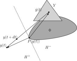
(a) Robust global attractiveness: condition (24).

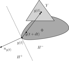
(b) Robust control invariance: condition (25).

Figure 6: Geometric representation of conditions (24) and (25).

Based on the above lemma, we can rephrase Theorem IV.2 as follows.

Theorem IV.4

Using the controller $u(t)=\hat{\phi}(sgn(x(t)))$ as in (17) we have that the vector $0$ is attainable by $x(t)$.

V Derivation of the main results

V-A Proof of Theorem IV.1

This proof is derived in the context of Lyapunov stochastic stability theory [20]. We start by observing that using $u(t)=\hat{\phi}(z(t))$ we have:

$$\dot{z}(t)=B\hat{\phi}(z(t))-v(t).$$ (26)

Consider a candidate Lyapunov function $V(z(t))=\frac{1}{2}z^{T}(t)z(t)$. The idea is to show that $\mathbb{E}[\dot{V}(z(t))]<0$ for all $t\geq 0$. Actually, the theory establishes that if the last condition holds true, then $V(z(t))$ is a supermartingale and therefore by the martingale convergence theorem $\lim_{t\rightarrow\infty}V(z(t))=0$ w.p.1 (almost surely). To see that $\mathbb{E}[\dot{V}(z(t))]<0$ is true, observe that from (15) we have

$$\mathbb{E}[\dot{V}(z(t))] = \mathbb{E}[z^{T}(t)\dot{z}(t)]$$

$$= \mathbb{E}[z^{T}(t)\Delta u(t)]-\mathbb{E}[z^{T}(t)B^{\dagger}\Delta v(t)]$$

$$= \mathbb{E}[z^{T}(t)sat(-z(t))]<0,$$

where condition $\mathbb{E}[z^{T}(t)B^{\dagger}\Delta v(t)]=0$ is a direct consequence of the assumption that $\Delta v(t)$ is independent of $x(t)$ and $y(t)$. But the above condition implies that $\lim_{t\rightarrow\infty}V(z(t))=0$ w.p.1 and therefore also $\lim_{t\rightarrow\infty}z(t)=0$ w.p.1. So far we have proved the first part of the statement, i.e., that the dynamic system (26) converges to zero w.p.1. For the second part, after integrating dynamics (15), we have

$$\lim_{t\rightarrow\infty}\frac{\int_{0}^{t}[\Delta u(\tau)-B^{\dagger}\Delta v(\tau)]d\tau}{t}=\lim_{t\rightarrow\infty}\frac{z(t)-z(0)}{t}=0.$$

This last condition together with the assumption $v_{nom}:=\lim_{t\rightarrow\infty}\bar{v}(t)$ yields

$$\lim_{t\rightarrow\infty}\frac{\int_{0}^{t}B^{\dagger}\Delta v(\tau)d\tau}{t}=\lim_{t\rightarrow\infty}\frac{\int_{0}^{t}\Delta u(\tau)d\tau}{t}=0$$

from which we can conclude $\lim_{t\rightarrow\infty}\bar{u}(t)=\lim_{t\rightarrow\infty}\frac{\int_{0}^{t}u_{nom}+\Delta u(\tau)d\tau}{t}=u_{nom}$ as claimed in the statement.

V-B Proof of Theorem IV.2

Consider a candidate Lyapunov function $V(x(t))=\frac{1}{2}x^{T}(t)x(t)$. The idea is to show that $\mathbb{E}[\dot{V}(x(t))]<0$ for all $t\geq 0$. For this to be true, it must be

$$\mathbb{E}[\dot{V}(x(t))] = \mathbb{E}[x^{T}(t)\dot{x}(t)]$$

$$= \mathbb{E}[x^{T}(t)Bu(t)]-\mathbb{E}[x^{T}(t)v(t)]$$

$$= \mathbb{E}[x^{T}(t)Bu_{nom}]+\mathbb{E}[x^{T}(t)B\Delta u(t)]-\mathbb{E}[x^{T}(t)v_{nom}]-\underbrace{\mathbb{E}[x^{T}(t)\Delta v(t)]}_{=0}$$

$$= \mathbb{E}[x^{T}(t)B\Delta u(t)]<0.$$

where condition $\mathbb{E}[x^{T}(t)\Delta v(t)]=0$ is a direct consequence of Assumption 4. But the above condition $\mathbb{E}[x^{T}(t)B\Delta u(t)]<0$ is satisfied since $B\Delta u(t)=-\delta sgn(x)$, which in turn implies

$$\mathbb{E}[x^{T}(t)B\Delta u(t)]=\mathbb{E}[-\delta\|x(t)\|_{1}]<0.$$

Then we obtain that $\lim_{t\rightarrow\infty}V(x(t))=0$ w.p.1 and therefore also $\lim_{t\rightarrow\infty}x(t)=0$ w.p.1 and this concludes the proof.

V-C Proof of Theorem IV.3

We first prove that (21) implies (22). Invoking the discrete time reformulation of Lemma III.1, we can infer that $\lim_{k\rightarrow\infty}\frac{x_{k}-x_{0}}{k}=0$ w.p.1. implies $\lim_{k\rightarrow\infty}\bar{a}_{k}\in C(v_{nom}),\,\mbox{w.p.1}$. Observing that $\bar{y}_{k}=\frac{x_{k}-x_{0}}{k}$ then we can conclude that $\lim_{k\rightarrow\infty}\bar{y}_{k}=0$ w.p.1 implies $\lim_{k\rightarrow\infty}\bar{a}_{k}\in C(v_{nom}),\,\mbox{w.p.1}$.

We now prove that using the controller $u_{k}=\hat{\phi}(sgn(x_{k}))$ as in (20) then (21) holds true. To see this, let us invoke the approachability principle in Lemma IV.1 and observe that a sufficient condition for approachability of $\bar{y}_{k}$ to $0$ is $\bar{y}^{T}_{k}y_{k+1}\leq 0$ for all $k$. This is evident if we take set $\Phi$ including only the zero vector, $\Phi=\{0\}$, and thus $P(\bar{y}_{k})=0$ in (19). For the present case, using the definition of $y_{k}$, condition $\bar{y}^{T}_{k}y_{k+1}\leq 0$ would be $\frac{1}{k}\left(x_{k}-x_{0}\right)^{T}\left(x_{k+1}-x_{k}\right)\leq 0$, which implies $(x_{k}-x_{0})^{T}B\Delta u_{k}-(x_{k}-x_{0})^{T}\Delta v_{k}\leq 0$ for all $k$. Taking the expectation, from Assumption 4 we know that $\mathbb{E}[(x_{k}-x_{0})^{T}\Delta v_{k}]=0$ and so we can write

$$\mathbb{E}[(x_{k}-x_{0})^{T}B\Delta u_{k}-(x_{k}-x_{0})^{T}\Delta v_{k}] = \mathbb{E}[(x_{k}-x_{0})^{T}B\Delta u_{k}]$$

$$= \mathbb{E}[(x_{k}-x_{0})^{T}B(-\delta B^{\dagger}sgn(x_{k}-x_{0}))]\leq 0.$$

From the above condition we derive that $\bar{y}^{T}_{k}y_{k+1}\leq 0$ w.p.1 for all $k$ and this concludes our proof.

V-D Proof of Theorem IV.4

Let us invoke the attainability principle in Lemma IV.2 and observe that a sufficient condition for $x(t)$ to attain $0$ w.p.1 is that

$$\mathbb{E}[x^{T}(t)\dot{x}(t)]<0, x(t)\not=0$$ (27)

$$\mathbb{E}[\dot{x}(t)]=0, x(t)=0.$$ (28)

This is evident if we take set $\Phi$ including only the zero vector, $\Phi=\{0\}$, and thus $P(x(t))=0$ in (24) and (25). Now, observe that condition (27) is equivalent to condition $\mathbb{E}[\dot{V}]<0$ used in the proof of Theorem IV.2. Condition (28) is also satisfied as $sgn(0)=0$ and this concludes our proof.

VI Numerical illustrations

Consider a $3$ player coalitional TU game, so $m=7$, with values of coalitions in the following intervals:

$$v(\{1\})\in[0,4],~{}v(\{2\})\in[0,4],~{}v(\{3\})\in[0,4],$$

$$v(\{1,2\})\in[0,4],~{}v(\{1,3\})\in[0,6],$$

$$v(\{2,3\})\in[0,7],~{}v(\{1,2,3\})\in[0,12].$$

The convex set $\mathcal{V}$ is then a hyperbox characterized by the above intervals. From Assumption 3, the planner knows the long run average game, i.e., $\lim_{t\rightarrow\infty}\bar{v}(t)=v_{nom}$. Without loss of generality we take the balanced nominal game be as $v_{nom}=[1~{}2~{}3~{}4~{}5~{}6~{}10]^{T}$. In other words, during the simulations we randomize the instantaneous games $v(t)\in\mathcal{V}$ so that it satisfies the average behavior given by:

$$\lim_{t\rightarrow\infty}\frac{1}{t}\int_{0}^{t}v(\tau)d\tau=v_{nom}.$$ (29)

Next, we describe an algorithm to generate $\mathbb{P}\in\Delta(\mathcal{V})$ and therefore $v(t)\in\mathcal{V}$ such that the above condition holds true.

Algorithm
Input: Set $\mathcal{V}$ and value $v_{nom}$.
Output: Probability function $\mathbb{P}\in\Delta(\mathcal{V})$ to generate $v(t)\in\mathcal{V}$.
$\quad 1:$ Initialize Generate $m$ random points, $r_{i}\in\mathcal{V}\subset\mathbb{R}^{m},~{}i=1,2,\cdots,m$,
$\quad 2:$ Solve $R.p=v_{nom}$, with $R=[r_{1},~{}r_{2},\cdots~{}r_{m}]$,
$\quad 3:$ If $p\geq 0$ and ${\mathbf{1}^{T}p}>0$, then go to (4) else go to (1),
$\quad 4:$ Rescale $R$ as $R=\left(\mathbf{1}^{T}p\right)R$ and $p$ as $p=\frac{p}{\left(\mathbf{1}^{T}p\right)}$,
$\quad 5:$ If $r_{i}\in\mathcal{V},~{}i=1,2,\cdots,m$, then go to (6) else go to (1).
$\quad 6:$ STOP

By construction, $v_{nom}$ is in the relative interior of the convex hull generated by the columns of the matrix $R$. If an instance of the game $v(t)$ is chosen as $r_{i}$ with probability $p_{i}$ from the pair $(R,p)$, Assumption 3 is satisfied. For simulations we ran the algorithm $10$ times to generate $10$ $(R,p)$ pairs in $\mathcal{V}$. Further, from each pair $(R,p)$ we take $100,000$ random selections (using Matlab randsrc function) to realize $v(t)$. The step size is set to $\Delta=0.05$. The results are averaged over the $10$ pairs. The nominal choice of allocations and surplus is taken as $u_{\text{nom}}=[2.5~{}3~{}4.5~{}1.5~{}1~{}1.5~{}1.5~{}2~{}1.5]^{T}$. It can be verified that $Bu_{\text{nom}}=v_{\text{nom}}$.

Full information case: The saturation thresholds $\Delta u^{min}$ and $\Delta u^{max}$ are chosen so as to ensure $u(t)\in U$. This condition translates into $U_{\text{min}}\leq u_{\text{nom}}+sat_{[\Delta u^{min},~{}\Delta u^{max}]}\leq U_{\text{max}}$. Denote $\mathbf{1}$ as a vector with all entries equal to 1. For the instantaneous game a negative allocation/surplus is not allowed, so $U_{min}\geq 0\cdot\mathbf{1}$. Further, an allocation/surplus greater than the value of grand coalition is not allowed, so $U_{max}\leq v_{nom}(N)\cdot\mathbf{1}$. For the given game parameters, we see that the lower and upper thresholds for the saturation function are $-1$ and $5.5$, respectively. Next, we present the performance results of the robust control law given by equation (16). From Theorem IV.1, $\lim_{t\rightarrow\infty}{z}(t)$ converges to zero w.p.1 and as a result $\lim_{t\rightarrow\infty}\frac{x(t)-x(0)}{t}$ converges to zero. Fig. 7(a) illustrates this behavior for the first component of coalition $\{1,2\}$. Further, by Corollary IV.1, the same control law ensures that the average allocations converge to the nominal allocations in the long run, in other words $\lim_{t\rightarrow\infty}\bar{a}(t)=a_{nom}$ and Fig. 7(b) illustrates this behavior.

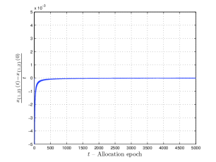
(a) Plot of $\frac{x_{\{1,2\}}(t)-x_{\{1,2\}}(0)}{t}$

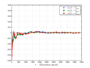
(b) Plot of $\lim_{t\rightarrow\infty}\bar{a}(t)-a_{nom}$

Figure 7: Performance of the control law given by (16).

Partial information case: The choice of $\delta$ is crucial so as to ensure $u(t)\in U$. This condition translates to $U_{\text{min}}\leq u_{\text{nom}}+\delta B^{\dagger}sgn(x)\leq U_{\text{max}}$. We observe $-\sum_{j}|B^{\dagger}_{ij}|\leq\left(B^{\dagger}sgn(x)\right)_{i}\leq\sum_{j}|B^{\dagger}_{ij}|$. A conservative estimate of $\delta$ is obtained as $U_{min}\leq{u_{nom}}\pm\delta\max_{i}\{\sum_{j}|B^{\dagger}_{ij}|\}\leq U_{max}$. For $m=7$, we have $\max_{i}\{\sum_{j}|B^{\dagger}_{ij}|\}=2.11$. For the instantaneous game a negative allocation/surplus is not allowed, so $U_{min}\geq 0.\mathbf{1}$. Furthermore, an allocation/surplus greater than the value of grand coalition is not allowed, so $U_{max}\leq v_{nom}(N).\mathbf{1}$. We chose $\delta=1$, which satisfies the above stated requirements.

(a) Plot of $\frac{x_{\{1,2\}}(t)-x_{\{1,2\}}(0)}{t}$

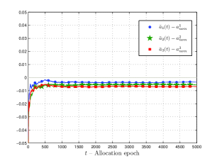
(b) Plot of $\lim_{t\rightarrow\infty}\bar{a}(t)-a_{nom}$

Figure 8: Performance of the control law given by (17).

Next, we present performance results of the robust control law given by equation (17). From Theorem IV.2, $x(t)$ converges to zero in probability with a specific choice of control law and as a result $\lim_{t\rightarrow\infty}\frac{x(t)-x(0)}{t}$ converges to zero. Fig. 8(a) illustrates this behavior for the first component of coalition $\{1,2\}$. Further, by Corollary IV.2, the same control law ensures that the average allocations converge to the core $C(v_{nom})$ and from equation (17) it is clear that the instantaneous allocations lie in a neighborhood of nominal allocations. As a result there is uncertainty in the convergence of average allocations towards nominal allocations on the long run and Fig. 8(b) illustrates this behavior.

VII Conclusions

In this paper we studied dynamic cooperative games where at each instant of time the value of each coalition of players is unknown but varies within a bounded polyhedron. With the assumption that the average value of each coalition in the long run is known with certainty, we presented robust allocations schemes, which converge to the core, under two informational settings. We proved the convergence of both allocation rules using Lyapunov stochastic stability theory. Furthermore, we established connections of Lyapunov stability theory to concepts of approachability and attainability. The control laws or allocation schemes are derived on the premise that the GD knows a priori, the nominal allocation vector. If this information is not available then the problem can be treated as a learning process where the GD is trying to learn the (balanced) nominal game from the instantaneous games. The allocation rules designed in this paper assure stability of the coalitions in average, and as a result capture patience and expectations of the players in an integral sense. The modeling aspects of generic dynamic coalitional games are open questions at this point of time.

References

- [1] S.Z. Alparslan Gök, S. Miquel, and S. Tijs, “Cooperation under interval uncertainty”, Mathematical Methods of Operations Research, vol. 69, no. 1, 2009, pp. 99–109.
- [2] T. Arnold., U. Schwalbe, “Dynamic coalition formation and the core”, Journal of Economic Behavior and Organization, vol. 49, 2002, pp. 363–380.
- [3] D. Bauso, F. Blanchini and R. Pesenti, “Optimization of Long-run Average-flow Cost in Networks with time-varying unknown demand”, IEEE Transactions on Automatic Control, vol. 55, no. 1, pp. 20-31, 2010.
- [4] D. Bauso, E. Lehrer, and E. Solan, “Attainability in Repeated Games with Vector Payoffs”, arXiv:1201.6054v1, 29 Jan 2012.
- [5] D. Bauso and P. V. Reddy, “Learning for allocations in the long-run average core of dynamical cooperative TU Games”, in Proc. of the 48th Annual Allerton Conference on Communication, Control, and Computing, University of Illinois, USA, Oct. 2010, pp. 1165-1170.
- [6] D. Bauso and P. V. Reddy, “Robust allocation rules in dynamical cooperative TU Games”, in Proc. of the 49th IEEE Conf. on Decision and Control, Atlanta, Georgia, USA, Dec 2010, pp. 1504–1509.
- [7] D. Bauso and J. Timmer, “Robust Dynamic Cooperative Games”, International Journal of Game Theory, vol. 38, no. 1, 2009, pp. 23–36.
- [8] D. P. Bertsekas and I. B. Rhodes, “On the Minimax Reachability of Target Sets and Target Tubes”, Automatica, vol. 7, pp. 233–241, March 1971.
- [9] D. Blackwell, “An analog of the minimax theorem for vector payoffs”, Pacific J. Math., vol. 6, no. 1, 1956, pp. 1–8.
- [10] F. Blanchini, “Set invariance in control – a survey”, Automatica, vol 35, no. 11, 1999, pp. 1747–1768.
- [11] L. Carpente, B. Casas-M ndez, I. Garc a-Jurado and A. van den Nouweland “Coalitional Interval Games for Strategic Games in Which Players Cooperate”, Theory and Decision, vol. 65, no. 3, 2008, pp. 253-269.
- [12] J.C. Cesco, “A convergent transfer scheme to the core of a TU-game”, Revista de Matemáticas Aplicadas, vol. 19, no. 1-2, 1998, pp. 23–35.
- [13] J.A. Filar and L.A. Petrosjan, “Dynamic Cooperative Games”, International Game Theory Review vol. 2, no. 1, 2000, pp. 47–65.
- [14] A.F. Filippov, “Differential equations with discontinuous right-hand side”, Amer. Math. Soc. Transl. (Orig. in Russian in Math. Sbornik 5 pp.99-127 (1960)) vol. 42, 1964, pp. 199-231.
- [15] J. H. Grotte, “Dynamics of cooperative games”, International Journal of Game Theory, vol. 5, no. 1, 1976, pp. 27–64.
- [16] A. Haurie, “On some Properties of the Characteristic Function and the Core of a Multistage Game of Coalitions”, IEEE Transactions on Automatic Control, vol. 20, no. 2, 1975, pp. 238–241.
- [17] L. Kranich, A. Perea, H. Peters, “Core concepts in dynamic TU games”, International Game Theory Review, vol. 7, 2005, pp. 43–61.
- [18] E. Lehrer, “Allocation Processes in Cooperative Games”, International Journal of Game Theory, vol. 31, 2002, pp. 341–351.
- [19] E. Lehrer, E. Solan, and D. Bauso, “Repeated Games over Networks with Vector Payoffs: The Notion of Attainability”, in Proc. of the Int. Conf. on NETwork Games, COntrol and OPtimization (NetGCooP 2011), 12-14 Oct. 2011, Paris.
- [20] K. A. Loparo, X. Feng, “Stability of stochastic systems”, In The Control Handbook. CRC Press, 1996.
- [21] W. Saad, Z. Han, M. Debbah, A. Hjørungnes, T. Başar, “Coalitional game theory for communication networks: A tutorial”, IEEE Signal Processing Magazine, Special Issue on Game Theory, vol. 26, no. 5, 2009, pp. 77–97.
- [22] A. Sengupta, K. Sengupta, “A property of the core”, Games and Economic Behavior, vol. 12, 1996, pp. 266–273.
- [23] J. Suijs and P. Borm, “Stochastic Cooperative Games: Superadditivity, Convexity, and Certainty Equivalents”, Games and Economic Behavior, vol. 27, no. 2, 1999, pp. 331–345.
- [24] J. Timmer, P. Borm, and S. Tijs, “On three Shapley-like solutions for cooperative games with random payoffs”, International Journal of Game Theory, vol. 32, 2003, pp. 595–613.
- [25] J. von Neumann, and O. Morgenstern, Theory of Games and Economic Behavior, Princeton, NJ: Princeton Univ. Press, Sept. 1944.
- [26] L. A. Wolsey and G. L. Nemhauser, “Integer and Combinatorial Optimization”, Wiley-Interscience, June 1988.
- [27] J. D. Williams, Probability with Martingales, Cambridge, U.K: Cambridge Univ. Press, Feb. 1991.