The Fourier U(2) Group and Separation of Discrete Variables

The Fourier U(2) Group and Separation
of Discrete Variables

Kurt Bernardo WOLF ^† and Luis Edgar VICENT ^‡

K.B. Wolf and L.E. Vincent

^† Instituto de Ciencias Físicas, Universidad Nacional Autónoma de México,
^† Av. Universidad s/n, Cuernavaca, Mor. 62210, México bwolf@fis.unam.mx http://www.fis.unam.mx/~bwolf/

^‡ Deceased

Received February 19, 2011, in final form May 26, 2011; Published online June 01, 2011

The linear canonical transformations of geometric optics on two-dimensional screens form the group Sp($4,\Re$), whose maximal compact subgroup is the Fourier group $\hbox{\sf U($2$)}_{\scriptscriptstyle\rm F}$; this includes isotropic and anisotropic Fourier transforms, screen rotations and gyrations in the phase space of ray positions and optical momenta. Deforming classical optics into a Hamiltonian system whose positions and momenta range over a finite set of values, leads us to the finite oscillator model, which is ruled by the Lie algebra so($4$). Two distinct subalgebra chains are used to model arrays of $N^{2}$ points placed along Cartesian or polar (radius and angle) coordinates, thus realizing one case of separation in two discrete coordinates. The $N^{2}$-vectors in this space are digital (pixellated) images on either of these two grids, related by a unitary transformation. Here we examine the unitary action of the analogue Fourier group on such images, whose rotations are particularly visible.

discrete coordinates; Fourier U(2) group; Cartesian pixellation; polar pixellation

20F28; 22E46; 33E30; 42B99; 78A05; 94A15

1 Introduction

The real symplectic group Sp($4,\Re$) of linear canonical transformations is widely used in paraxial geometric optics [2, Part 3] on two-dimensional screens, and in classical mechanics with quadratic potentials. Its maximal compact subgroup is the Fourier group $\hbox{\sf U($2$)}_{\scriptscriptstyle\rm F}=\hbox{\sf U($1$)}_{\scriptscriptstyle\rm F}\otimes\hbox{\sf SU($2$)}_{\scriptscriptstyle\rm F}$ [3, 4]. These are classical Hamiltonian systems with two coordinates of position $(q_{x},q_{y})\in\Re^{2}$, and two coordinates of momentum $(p_{x},p_{y})\in\Re^{2}$, which form the phase space $\Re^{4}$, and which are subject to linear canonical transformations that preserve the volume element. The central subgroup $\hbox{\sf U($1$)}_{\scriptscriptstyle\rm F}$ contains the fractional isotropic Fourier transforms, which rotate the planes $(q_{x},p_{x})$ and $(q_{y},p_{y})$ by a common angle. The complement group $\hbox{\sf SU($2$)}_{\scriptscriptstyle\rm F}$ contains anisotropic Fourier transforms that rotate the planes $(q_{x},p_{x})$ and $(q_{y},p_{y})$ by opposite angles; it also contains joint rotations of the $(q_{x},q_{y})$ and $(p_{x},p_{y})$ planes; and thirdly, gyrations, which ‘cross-rotate’ the planes $(q_{x},p_{y})$ and $(q_{y},p_{x})$. The rest of the Sp($4,\Re$) transformations shear or squeeze phase space, as free flights and lenses, or harmonic oscillator potential jolts.

This classical system can be quantized à la Schrödinger into paraxial wave or quantum models. Indeed, the group of canonical integral transforms was investigated early by Moshinsky and Quesne in quantum mechanics [5, 6], [7, Part 4] and by Collins in optics [8], and yielded the integral transform kernel that unitarily represents the (two-fold cover of the) group Sp($4,\Re$) on the Hilbert space ${\cal L}^{2}(\Re^{2})$. Yet it is the discrete version of this system which is of interest for its technological applications to sensing wavefields with ccd arrays. One line of research addresses the discretization of the integral kernel to a matrix and its computation using the fast FFT algorithm [9, 10, 11, 12]. This has the downside that the kernel matrices are in general not unitary, and thus no longer represent the group – non-compact groups can have only infinite-dimensional unitary representations [13].

We have developed a ‘finite quantization’ process to pass between classical quadratic Hamiltonian systems, to systems whose position and momentum coordinates are discrete and finite [14, 15, 16, 17, 18]. The set of values a discrete and finite coordinate can have is the spectrum of the generator of a compact subalgebra of u($2$), which is a deformation of the oscillator Lie algebra osc. When position space is two-dimensional, we use $\hbox{\sf so($4$)}=\hbox{\sf su($2$)}_{x}\oplus\hbox{\sf su($2$)}_{y}$ [18, 19, 20]. The purpose of this article is to elucidate the action of the Fourier group $\hbox{\sf U($2$)}_{\scriptscriptstyle\rm F}$ on the $N^{2}$-dimensional representation spaces of the algebra so($4$) that we use to realize pixellated images.

Previously we have analyzed and synthesized pixellated images on sensor arrays that follow Cartesian or polar coordinates [19, 20, 21]; here we investigate the action of the Fourier group on finite pixellated images arranged along these two coordinate systems, understood as one example of separation of coordinates in discrete, finite spaces. In order to present a reasonably self-contained review of our approach to two-dimensional finite systems, we must repeat developments that have appeared previously, which will be recognized by the citation of the relevant references. As research experience indicates however, each restatement of previous results yields a streamlined and better structured text, where the notation is unified and directed toward the economic statement of the solution to the problem at hand. In the present case, it is the action of the four-parameter Fourier group on Cartesian and polar-pixellated images.

The classical Fourier subgroup of paraxial optics on two-dimensional screens [4] is described in Section 2. To finitely quantize this, we review the one-dimensional case, where u($2$) is used to model the finite harmonic oscillator [14, 17, 18] in Section 3. The ascent to two-dimensional finite systems, Cartesian and polar, occupies the longer Section 4. There, under the ægis of so($4$) we describe its finite position space separated in Cartesian [16] and in polar [19] coordinates, together with the two-parameter subgroups of the Fourier group that are within so($4$) for each coordinate system. The new developments begin in Section 5, where we import the continuous group of rotations on images pixellated along Cartesian coordinates from their natural action on the polar pixellation. This serves to complete the action of the $\hbox{\sf U($2$)}_{\scriptscriptstyle\rm F}$ Fourier group on Cartesian screens in Section 6. To translate the action of this group onto polar screens, we recall in Section 7 the unitary transformation between Cartesian and polar-pixellated screens [20], thus finding the representation of the Fourier group on the circular grid as well. Finally, in Section 8 we offer some comments on the wider context in which we hope to place the separation of discrete coordinates in two dimensions.

2 The classical Fourier group

The classical oscillator is characterized by the Lie algebra osc of Poisson brackets between the oscillator Hamiltonian function $h(q,p):=\frac{1}{2}(p^{2}+q^{2})$ and the phase space coordinates of position $q$ and momentum $p$,

$$\{h,q\}_{\scriptscriptstyle\rm P}=-p,\qquad\{h,p\}_{\scriptscriptstyle\rm P}=q,\qquad\{q,p\}_{\scriptscriptstyle\rm P}:=1,$$ (2.1)

where 1 Poisson-commutes with all. The first two brackets are the geometric and dynamic Hamilton equations, while the last one actually defines the algebra of the system to be osc.

In two dimensions $(q_{x},q_{y})\in\Re^{2}$ and with the corresponding momenta $(p_{x},p_{y})\in\Re^{2}$, one can build ten independent quadratic functions

$$q_{i}q_{i^{\prime}},\qquad q_{i}p_{i^{\prime}},\qquad p_{i}p_{i^{\prime}},\qquad i,{i^{\prime}}\in\{x,y\},$$ (2.2)

that will close into the real symplectic Lie algebra sp($4,\Re$). Four linear combinations of them generate transformations that include the fractional Fourier transform (FT), which are of interest in optical image processing,

$$\hbox{isotropic FT \ }F_{0}:={\textstyle\frac{1}{4}}\left(p^{2}_{x}+p^{2}_{y}+q^{2}_{x}+q^{2}_{y}\right)=:\textstyle\frac{1}{2}(h_{x}+h_{y}),$$ (2.3)

$$\hbox{anisotropic FT \ }F_{1}:={\textstyle\frac{1}{4}}\left(p^{2}_{x}-p^{2}_{y}+q^{2}_{x}-q^{2}_{y}\right)=:\textstyle\frac{1}{2}(h_{x}-h_{y}),$$ (2.4)

$$\hbox{gyration \ }F_{2}:={\textstyle\frac{1}{2}}(p_{x}p_{y}+q_{x}q_{y}),$$ (2.5)

$$\hbox{rotation \ }F_{3}:={\textstyle\frac{1}{2}}(q_{x}p_{y}-q_{y}p_{x}).$$ (2.6)

Their Poisson brackets close within the set,

$$\{F_{1},F_{2}\}_{\scriptscriptstyle\rm P}=F_{3},\qquad\hbox{and cyclically},$$

$$\{F_{0},F_{i}\}_{\scriptscriptstyle\rm P}=0,\qquad i=1,2,3,$$

and characterize the Fourier Lie algebra $\hbox{\sf u($2$)}_{\scriptscriptstyle\rm F}=\hbox{\sf u($1$)}_{\scriptscriptstyle\rm F}\oplus\hbox{\sf su($2$)}_{\scriptscriptstyle\rm F}$, with $F_{0}$ central. This is the maximal compact subalgebra of (2.2), $\hbox{\sf u($2$)}_{\scriptscriptstyle\rm F}\subset\hbox{\sf sp($4,\Re$)}$ [4]. In Fig. 1 we show the transformations generated by (2.4)–(2.6) on the linear space of the su($2$) algebra, which leaves invariant the spheres $F^{2}_{1}+F^{2}_{2}+F^{2}_{3}=F^{2}_{0}$.

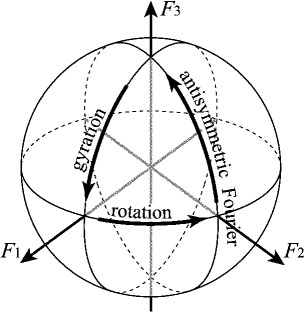
Figure 1: Action of the Fourier group on the sphere (from [22]).

The Lie algebra u($2$) and group U($2$) will appear in several guises, so it is important to distinguish their ‘physical’ meaning. The classical Fourier group $\hbox{\sf U($2$)}_{\scriptscriptstyle\rm F}$ of linear optics will be matched by a ‘Fourier–Kravchuk’ group $\hbox{\sf U($2$)}_{\scriptscriptstyle\rm K}$ acting on the position space of finite ‘sensor’ arrays in the finite oscillator model. In one dimension, this model is based on the algebra u($2$), whose generators are position, momentum, and energy; while in two, the algebra is $\hbox{\sf su($2$)}_{x}\oplus\hbox{\sf su($2$)}_{y}=\hbox{\sf so($4$)}$. In all, the well-known properties of $\hbox{\sf su($2$)}=\hbox{\sf so($3$)}$ will of use [23].

3 Finite quantization in one dimension

The usual Schrödinger quantization $(q\mapsto\bar{Q}=q\cdot$, $p\mapsto\bar{P}=-{\rm i}\eta{\rm d}/{\rm d}q)$ of the phase space coordinates leads to the paraxial model of wave optics (for the reduced wavelength $\eta=\lambda/2\pi$) or to oscillator quantum mechanics (for $\eta=\hbar$). In one dimension, (2.2) yields the three generators of the (double cover of the) group Sp($2,\Re$) of canonical integral transforms [5] acting on functions – continuous infinite signals – in the Hilbert space ${\cal L}^{2}(\Re)$. In two dimensions, the Schrödinger quantization of (2.2) yields the generators of Sp($4,\Re$), and its Fourier subgroup is generated by the quadratic Schrödinger operators $\bar{F}_{0}$, $\bar{F}_{1}$, $\bar{F}_{2}$, $\bar{F}_{3}$ corresponding to (2.3)–(2.6), that we indicate with bars, and are up-to-second order differential operators acting on the Hilbert space. Finite quantization on the other hand, asigns self-adjoint $N\times N$ matrices $q\mapsto Q$, $p\mapsto P$ to the coordinates of phase space.

Since the oscillator algebra is noncompact, it cannot have a faithful representation by finite self-adjoint matrices [13]; we must thus deform the four-generator osc into a compact algebra, of which there is a single choice: u($2$). We should keep the geometry and dynamics of the harmonic oscillator contained in the two Hamilton equations in (2.1), with commutators ${\rm i}[\,\cdot\,,\,\cdot\,]$ in place of the Poisson brackets $\{\cdot,\cdot\}_{\scriptscriptstyle\rm P}$, and in place of the oscillator Hamiltonian $h$, a matrix $K$ added with some constant times the unit matrix. We call $K$ the pseudo-Hamiltonian. The third – and fundamental – commutator $[Q,P]$ will then give back $K$. In [14] we proposed the assignments of self-adjoint $N\times N$ matrices given by the well-known irreducible representations of the Lie algebra su($2$) of spin $j$, thus of dimension $N=2j+1$, where the matrix representing position is chosen diagonal. Using the generic notation $\{J_{1},J_{2},J_{3}\}$ for generators of su($2$), the matrices are

$$\hbox{position:}\quad q\mapsto Q=J_{1},$$

$$\qquad Q_{m,m^{\prime}}=m\delta_{m,m^{\prime}},\qquad m,m^{\prime}\in\{-j,-j+1,\ldots,j\},$$ (3.1)

$$\hbox{momentum:}\quad p\mapsto P=J_{2},$$

$$\qquad P_{m,m^{\prime}}=-{\rm i}\textstyle\frac{1}{2}\sqrt{{(j-m)(j+m+1)}}\delta_{m+1,m^{\prime}}+{\rm i}\textstyle\frac{1}{2}\sqrt{{(j+m)(j-m+1)}}\delta_{m-1,m^{\prime}},$$ (3.2)

$$\hbox{pseudo-energy:}\quad K=J_{3},\qquad\hbox{energy:}\quad h\mapsto H:=K+(j+\textstyle\frac{1}{2})1,$$

$$\qquad K_{m,m^{\prime}}=\textstyle\frac{1}{2}\sqrt{{(j-m)(j+m+1)}}\delta_{m+1,m^{\prime}}+\textstyle\frac{1}{2}\sqrt{{(j+m)(j-m+1)}}\delta_{m-1,m^{\prime}}.$$ (3.3)

The commutation relations of these matrices are

$$[K,Q]=-{\rm i}P,\qquad[K,P]={\rm i}Q,\qquad[Q,P]=-{\rm i}K,$$

$$\hbox{i.e.},\qquad[J_{1},J_{2}]=-{\rm i}J_{3},\qquad\hbox{and cyclically}.$$ (3.4)

The central generator 1 of osc is corresponded with the unit $N\times N$ matrix that generates a U($1$) central group of multiplication by overall phases. This completes the algebra u($2$) realized by matrices acting on the linear space ${\cal C}^{N}$ of complex $N$-vectors.

The spectra $\Sigma$ of the matrices $Q$ of position $\{q\}$, $P$ of momentum $\{\varpi\}$, and $K$ of pseudo-energy $\{\kappa\}$ are thus discrete and finite,

$$\Sigma(Q)=\Sigma(P)=\Sigma(K)=\{-j,-j+1,\ldots,j\},$$

with $j$ integer or half-integer. We define the mode number as $n:=\kappa+j\in\{0,1,\ldots,2j\}$, and energy is $n+\textstyle\frac{1}{2}$. The Lie group generated by $\{1;Q,P,K\}$ is the U($2$) group of linear unitary transformations of ${\cal C}^{N}$. Finally, the sum of squares of these matrices on ${\cal C}^{N}$ is the Casimir invariant

$$C:=Q^{2}+P^{2}+K^{2}=j(j+1)1.$$

In Dirac notation, ${\cal C}^{N}$ is a spin-$j$ u($2$) representation, where the eigenstates of position $q$ and of mode $n=\kappa+j$ satisfy

$$Q\,|q\rangle_{\!{\scriptscriptstyle\rm 1}}=q\,|q\rangle_{\!{\scriptscriptstyle\rm 1}},\qquad K\,|n\rangle_{\!{\scriptscriptstyle\rm 3}}=(n-j)\,|n\rangle_{\!{\scriptscriptstyle\rm 3}},\qquad q|_{-j}^{j},\qquad n|_{0}^{2j}.$$ (3.5)

The position eigenvectors $\,|q\rangle_{\!{\scriptscriptstyle\rm 1}}$ form a Kronecker basis for ${\cal C}^{N}$ where the components of $\,|n\rangle_{\!{\scriptscriptstyle\rm 3}}$ will be provided, from (3.3), by a three-term relation, i.e., a difference equation that is satisfied by the Wigner little-d functions [23] for $\kappa=n-j$. (The reader may be disconcerted for having $J_{1}$ diagonal, whereas almost universally $J_{3}$ is declared the diagonal matrix; formulas obtained by permuting $1\mapsto 2\mapsto 3\mapsto 1$ are unchanged.) The overlaps between the two bases in (3.5) are the finite oscillator wavefunctions,

$$\Psi_{n}(q):=\!\!\!\!\phantom{{|}e}_{{\scriptscriptstyle\rm 1}}^{{}\!\!}\!\langle{q}|{n}\rangle_{{\scriptscriptstyle\rm 3}}=d^{j}_{n-j,q}\big{(}\textstyle\frac{1}{2}\pi\big{)}=\Psi_{q+j}(n-j)$$ (3.6)

$$\phantom{\Psi_{n}(q)}{}\,=\frac{(-1)^{n}}{2^{j}}\sqrt{\left({2j\atop n}\right)\left({2j\atop q+j}\right)}K_{n}\big{(}q+j;\textstyle\frac{1}{2},2j\big{)}.$$ (3.7)

This overlap is expressed here [24] in terms of the square root of a binomial coefficient in $q$, which is a discrete version of the Gaussian, and a symmetric Kravchuk polynomial of degree $n$, $K_{n}(q)\equiv K_{n}(q;\textstyle\frac{1}{2},N-1)=K_{q}(n-j)$ [25]. We have called the $\Psi_{n}(q)$’s Kravchuk functions [14]; they form a real, orthonormal and complete basis for ${\cal C}^{N}$. The Lie exponential of the self-adjoint matrix $K$ generates the unitary U($1$) group of fractional Fourier–Kravchuk transforms, whose realization we shall indicate by $\hbox{\sf U($1$)}_{\scriptscriptstyle\rm K}$.

For future use we give the general expression of the Wigner little-$d$ functions for angles $\beta\in[0,\pi]$ as a trigonometric polynomial [13, 23]

$$d^{j}_{m^{\prime},m}(\beta)=\sqrt{(j+m^{\prime})!(j-m^{\prime})!(j+m)!(j-m)!}$$

$$\phantom{d^{j}_{m^{\prime},m}(\beta)=}{}\times\sum_{k}\frac{(-1)^{m^{\prime}-m+k}(\cos\textstyle\frac{1}{2}\beta)^{2j+m-m^{\prime}-2k}(\sin\textstyle\frac{1}{2}\beta)^{m^{\prime}-m+2k}}{k!(j+m-k)!(m^{\prime}-m+k)!(j-m^{\prime}-k)!}$$ (3.8)

$$\phantom{d^{j}_{m^{\prime},m}(\beta)}{}=d^{j}_{m^{\prime},m}(-\beta)=(-1)^{m-m^{\prime}}d_{j-m,j-m^{\prime}}(\beta),$$ (3.9)

where due to the denominator factorials, the summation extends over the integer range of $\max(0,m-m^{\prime})\leq k\leq\min(j-m^{\prime},j+m)$; for $m-m^{\prime}>0$ the reflection formulas (3.9) apply.

4 Two-dimensional systems

The two-dimensional classical oscillator algebra $\hbox{\sf osc}_{2}$ is sometimes taken to consist of the Poisson brackets between $1$, $q_{x}$, $q_{y}$, $p_{x}$, $p_{y}$, and $h_{x}$, $h_{y}$; and sometimes an angular momentum $m=q_{1}p_{2}-q_{2}p_{1}$ is included, Poisson-commuting with the total Hamiltonian $h=h_{x}+h_{y}$. The finite quantization of two-dimensional systems deforms $\hbox{\sf osc}_{2}$ to the Lie algebra $\hbox{\sf su($2$)}\oplus\hbox{\sf su($2$)}=\hbox{\sf so($4$)}$ in both cases. (The subalgebra of 1 need not concern us here.) To work comfortably with the six generators of so($4$), we consider the customary realization of $J_{i,i^{\prime}}=-J_{i^{\prime},i}$ by self-adjoint operators that generate rotations in the $(i,i^{\prime})$ planes, which obey the commutation relations

$$[J_{i,i^{\prime}},J_{k,k^{\prime}}]={\rm i}(\delta_{i^{\prime},k}J_{i,k^{\prime}}+\delta_{i,k^{\prime}}J_{i^{\prime},k}+\delta_{k,i}J_{k^{\prime},i^{\prime}}+\delta_{k^{\prime},i^{\prime}}J_{k,i}),$$

that we summarize with the following pattern:

$$\vbox{\vbox{\hbox{}\vskip-10.8pt\vbox to19.91684pt{\vss\hbox to85.35826pt{\hfil$\displaystyle\hfill\framebox{\vbox to19.91684pt{\vfil\hbox to19.91684pt{\hfil$\displaystyle J_{1,2}$\hfil}\vfil}}\hskip 0.0pt\hbox{}\framebox{\vbox to19.91684pt{\vfil\hbox to19.91684pt{\hfil$\displaystyle J_{1,3}$\hfil}\vfil}}\hskip 0.0pt\hbox{}\framebox{\vbox to19.91684pt{\vfil\hbox to19.91684pt{\hfil$\displaystyle J_{1,4}$\hfil}\vfil}}\hskip 0.0pt\hbox{}$\hfil}\vss}\vskip-11.8pt\hbox{} \hbox{}\vskip-10.8pt\vbox to19.91684pt{\vss\hbox to85.35826pt{\hfil$\displaystyle\hfill\framebox{\vbox to19.91684pt{\vfil\hbox to19.91684pt{\hfil$\displaystyle J_{2,3}$\hfil}\vfil}}\hskip 0.0pt\hbox{}\framebox{\vbox to19.91684pt{\vfil\hbox to19.91684pt{\hfil$\displaystyle J_{2,4}$\hfil}\vfil}}\hskip 0.0pt\hbox{}$\hfil}\vss}\vskip-11.8pt\hbox{} \hbox{}\vskip-10.8pt\vbox to19.91684pt{\vss\hbox to85.35826pt{\hfil$\displaystyle\hfill\framebox{\vbox to19.91684pt{\vfil\hbox to19.91684pt{\hfil$\displaystyle J_{3,4}$\hfil}\vfil}}\hskip 0.0pt\hbox{}$\hfil}\vss}\vskip-11.8pt\hbox{}}}\ .$$ (4.1)

A generator $J_{i,i^{\prime}}$ has non-zero commutator with all those in its row $i$ and its column $i^{\prime}$ (reflected across the $i=i^{\prime}$ line); all its other commutators are zero. The asignments of position, momentum and pseudo-energy with the $\hbox{\sf su($2$)}=\hbox{\sf so($3$)}$ matrices (3.1)–(3.3) is

$${}\hskip-42.67912pt{}\vbox{\vbox{\hbox{}\vskip-10.8pt\vbox to19.91684pt{\vss\hbox to85.35826pt{\hfil$\displaystyle\hfill\framebox{\vbox to19.91684pt{\vfil\hbox to19.91684pt{\hfil$\displaystyle K$\hfil}\vfil}}\hskip 0.0pt\hbox{}\framebox{\vbox to19.91684pt{\vfil\hbox to19.91684pt{\hfil$\displaystyle{-}P$\hfil}\vfil}}\hskip 0.0pt\hbox{}$\hfil}\vss}\vskip-11.8pt\hbox{}\hbox{}\vskip-10.8pt\vbox to19.91684pt{\vss\hbox to85.35826pt{\hfil$\displaystyle\hfill\framebox{\vbox to19.91684pt{\vfil\hbox to19.91684pt{\hfil$\displaystyle Q$\hfil}\vfil}}\hskip 0.0pt\hbox{}$\hfil}\vss}\vskip-11.8pt\hbox{}}}{\qquad\hbox{\LARGE$=$}}\vbox{\vbox{\hbox{}\vskip-10.8pt\vbox to19.91684pt{\vss\hbox to85.35826pt{\hfil$\displaystyle\hfill\framebox{\vbox to19.91684pt{\vfil\hbox to19.91684pt{\hfil$\displaystyle J_{1,2}$\hfil}\vfil}}\hskip 0.0pt\hbox{}\framebox{\vbox to19.91684pt{\vfil\hbox to19.91684pt{\hfil$\displaystyle J_{1,3}$\hfil}\vfil}}\hskip 0.0pt\hbox{}$\hfil}\vss}\vskip-11.8pt\hbox{}\hbox{}\vskip-10.8pt\vbox to19.91684pt{\vss\hbox to85.35826pt{\hfil$\displaystyle\hfill\framebox{\vbox to19.91684pt{\vfil\hbox to19.91684pt{\hfil$\displaystyle J_{2,3}$\hfil}\vfil}}\hskip 0.0pt\hbox{}$\hfil}\vss}\vskip-11.8pt\hbox{}}}{\qquad\hbox{\LARGE$=$}}\vbox{\vbox{\hbox{}\vskip-10.8pt\vbox to19.91684pt{\vss\hbox to85.35826pt{\hfil$\displaystyle\hfill\framebox{\vbox to19.91684pt{\vfil\hbox to19.91684pt{\hfil$\displaystyle J_{3}$\hfil}\vfil}}\hskip 0.0pt\hbox{}\framebox{\vbox to19.91684pt{\vfil\hbox to19.91684pt{\hfil$\displaystyle{-}J_{2}$\hfil}\vfil}}\hskip 0.0pt\hbox{}$\hfil}\vss}\vskip-11.8pt\hbox{}\hbox{}\vskip-10.8pt\vbox to19.91684pt{\vss\hbox to85.35826pt{\hfil$\displaystyle\hfill\framebox{\vbox to19.91684pt{\vfil\hbox to19.91684pt{\hfil$\displaystyle J_{1}$\hfil}\vfil}}\hskip 0.0pt\hbox{}$\hfil}\vss}\vskip-11.8pt\hbox{}}}\ .$$

4.1 The Cartesian coordinate system

Passing from one to two dimensions can be achieved prima facie by building the direct sum algebra $\hbox{\sf su($2$)}_{x}\oplus\hbox{\sf su($2$)}_{y}$, which is accidentally equal to so($4$). This isomorphism is shown in patterns by

$${}\hskip-42.67912pt{}\vbox{\vbox{\hbox{}\vskip-10.8pt\vbox to19.91684pt{\vss\hbox to85.35826pt{\hfil$\displaystyle\hfill\framebox{\vbox to19.91684pt{\vfil\hbox to19.91684pt{\hfil$\displaystyle K^{{\lower 2.0pt\hbox{\tiny{\char 48\relax}}}}_{x}$\hfil}\vfil}}\hskip 0.0pt\hbox{}\framebox{\vbox to19.91684pt{\vfil\hbox to19.91684pt{\hfil$\displaystyle{}\!{-}P^{{\lower 2.0pt\hbox{\tiny{\char 48\relax}}}}_{x}$\hfil}\vfil}}\hskip 0.0pt\hbox{}$\hfil}\vss}\vskip-11.8pt\hbox{}\hbox{}\vskip-10.8pt\vbox to19.91684pt{\vss\hbox to85.35826pt{\hfil$\displaystyle\hfill\framebox{\vbox to19.91684pt{\vfil\hbox to19.91684pt{\hfil$\displaystyle Q^{{\lower 2.0pt\hbox{\tiny{\char 48\relax}}}}_{x}$\hfil}\vfil}}\hskip 0.0pt\hbox{}$\hfil}\vss}\vskip-11.8pt\hbox{}}}{\quad\hbox{\LARGE$\oplus$}\hskip-20.0pt}\vbox{\vbox{\hbox{}\vskip-10.8pt\vbox to19.91684pt{\vss\hbox to85.35826pt{\hfil$\displaystyle\hfill\framebox{\vbox to19.91684pt{\vfil\hbox to19.91684pt{\hfil$\displaystyle K^{{\lower 2.0pt\hbox{\tiny{\char 48\relax}}}}_{y}$\hfil}\vfil}}\hskip 0.0pt\hbox{}\framebox{\vbox to19.91684pt{\vfil\hbox to19.91684pt{\hfil$\displaystyle{}\!{-}P^{{\lower 2.0pt\hbox{\tiny{\char 48\relax}}}}_{y}$\hfil}\vfil}}\hskip 0.0pt\hbox{}$\hfil}\vss}\vskip-11.8pt\hbox{}\hbox{}\vskip-10.8pt\vbox to19.91684pt{\vss\hbox to85.35826pt{\hfil$\displaystyle\hfill\framebox{\vbox to19.91684pt{\vfil\hbox to19.91684pt{\hfil$\displaystyle Q^{{\lower 2.0pt\hbox{\tiny{\char 48\relax}}}}_{y}$\hfil}\vfil}}\hskip 0.0pt\hbox{}$\hfil}\vss}\vskip-11.8pt\hbox{}}}{\quad\hbox{\LARGE$=$}\hskip-30.0pt}\vbox{\vbox{\hbox{}\vskip-10.8pt\vbox to19.91684pt{\vss\hbox to199.16928pt{\hfil$\displaystyle\hfill\framebox{\vbox to19.91684pt{\vfil\hbox to51.21504pt{\hfil$\displaystyle K^{{\lower 2.0pt\hbox{\tiny{\char 48\relax}}}}_{x}+K^{{\lower 2.0pt\hbox{\tiny{\char 48\relax}}}}_{y}$\hfil}\vfil}}\hskip 0.0pt\hbox{}\framebox{\vbox to19.91684pt{\vfil\hbox to51.21504pt{\hfil$\displaystyle-P^{{\lower 2.0pt\hbox{\tiny{\char 48\relax}}}}_{x}-P^{{\lower 2.0pt\hbox{\tiny{\char 48\relax}}}}_{y}$\hfil}\vfil}}\hskip 0.0pt\hbox{}\framebox{\vbox to19.91684pt{\vfil\hbox to51.21504pt{\hfil$\displaystyle Q^{{\lower 2.0pt\hbox{\tiny{\char 48\relax}}}}_{x}-Q^{{\lower 2.0pt\hbox{\tiny{\char 48\relax}}}}_{y}$\hfil}\vfil}}\hskip 0.0pt\hbox{}$\hfil}\vss}\vskip-11.8pt\hbox{} \hbox{}\vskip-10.8pt\vbox to19.91684pt{\vss\hbox to199.16928pt{\hfil$\displaystyle\hfill\framebox{\vbox to19.91684pt{\vfil\hbox to51.21504pt{\hfil$\displaystyle Q^{{\lower 2.0pt\hbox{\tiny{\char 48\relax}}}}_{x}+Q^{{\lower 2.0pt\hbox{\tiny{\char 48\relax}}}}_{y}$\hfil}\vfil}}\hskip 0.0pt\hbox{}\framebox{\vbox to19.91684pt{\vfil\hbox to51.21504pt{\hfil$\displaystyle P^{{\lower 2.0pt\hbox{\tiny{\char 48\relax}}}}_{x}-P^{{\lower 2.0pt\hbox{\tiny{\char 48\relax}}}}_{y}$\hfil}\vfil}}\hskip 0.0pt\hbox{}$\hfil}\vss}\vskip-11.8pt\hbox{} \hbox{}\vskip-10.8pt\vbox to19.91684pt{\vss\hbox to199.16928pt{\hfil$\displaystyle\hfill\framebox{\vbox to19.91684pt{\vfil\hbox to51.21504pt{\hfil$\displaystyle K^{{\lower 2.0pt\hbox{\tiny{\char 48\relax}}}}_{x}-K^{{\lower 2.0pt\hbox{\tiny{\char 48\relax}}}}_{y}$\hfil}\vfil}}\hskip 0.0pt\hbox{}$\hfil}\vss}\vskip-11.8pt\hbox{}}}\ ,\quad{}$$ (4.2)

where the square super-index of all generators, $X^{{\lower 2.0pt\hbox{\tiny{\char 48\relax}}}}_{i}$, indicates the identification between the so($4$) generators $J_{i,i^{\prime}}$ with the Cartesian coordinates and observables.

Since the $x$-generators commute with the $y$-generators in (4.2), using (3.5) a Cartesian basis of positions and also a basis of modes can be simply defined as direct products $\displaystyle\,|q_{x},q_{y}\rangle_{\!{\scriptscriptstyle\rm 1\ }}^{{\lower 2.0pt\hbox{\tiny{\char 48\relax}}}}:=\,|q_{x}\rangle_{\!{\scriptscriptstyle\rm 1x}}\!\,|q_{y}\rangle_{\!{\scriptscriptstyle\rm 1y}}$ and $\displaystyle\,|n_{x},n_{y}\rangle_{\!{\scriptscriptstyle\rm 3\ }}^{{\lower 2.0pt\hbox{\tiny{\char 48\relax}}}}:=\,|n_{x}\rangle_{\!{\scriptscriptstyle\rm 3x}}\!\,|n_{y}\rangle_{\!{\scriptscriptstyle\rm 3y}}$,

$$Q^{{\lower 2.0pt\hbox{\tiny{\char 48\relax}}}}_{x}\,|q_{x},q_{y}\rangle_{\!{\scriptscriptstyle\rm 1}}^{{\lower 2.0pt\hbox{\tiny{\char 48\relax}}}}=q_{x}\,|q_{x},q_{y}\rangle_{\!{\scriptscriptstyle\rm 1}}^{{\lower 2.0pt\hbox{\tiny{\char 48\relax}}}},\qquad Q^{{\lower 2.0pt\hbox{\tiny{\char 48\relax}}}}_{y}\,|q_{x},q_{y}\rangle_{\!{\scriptscriptstyle\rm 1}}^{{\lower 2.0pt\hbox{\tiny{\char 48\relax}}}}=q_{y}\,|q_{x},q_{y}\rangle_{\!{\scriptscriptstyle\rm 1}}^{{\lower 2.0pt\hbox{\tiny{\char 48\relax}}}},$$ (4.3)

$$K^{{\lower 2.0pt\hbox{\tiny{\char 48\relax}}}}_{x}\,|n_{x},n_{y}\rangle_{\!{\scriptscriptstyle\rm 3}}^{{\lower 2.0pt\hbox{\tiny{\char 48\relax}}}}=(n_{x}-j)\,|n_{x},n_{y}\rangle_{\!{\scriptscriptstyle\rm 3}}^{{\lower 2.0pt\hbox{\tiny{\char 48\relax}}}},\qquad K^{{\lower 2.0pt\hbox{\tiny{\char 48\relax}}}}_{y}\,|n_{x},n_{y}\rangle_{\!{\scriptscriptstyle\rm 3}}^{{\lower 2.0pt\hbox{\tiny{\char 48\relax}}}}=(n_{y}-j)\,|n_{x},n_{y}\rangle_{\!{\scriptscriptstyle\rm 3}}^{{\lower 2.0pt\hbox{\tiny{\char 48\relax}}}},$$ (4.4)

where the pseudo-energy eigenvalues are $n_{i}-j=\kappa_{i}|_{-j}^{j}$. The two-dimensional finite oscillator wavefunctions in Cartesian coordinates are thus given as a product of two $\Psi_{n}(q)$’s from (3.6), (3.7),

$$\Psi^{\lower 2.0pt\hbox{\tiny{\char 48\relax}}}_{n_{x},n_{y}}(q_{x},q_{y})=\phantom{{|}e}_{{\scriptscriptstyle\rm 1}}^{{}\!\!{\lower 2.0pt\hbox{\tiny{\char 48\relax}}}}\!\langle{q_{x},q_{y}}|{n_{x},n_{y}}\rangle_{{\scriptscriptstyle\rm 3}}^{{\lower 2.0pt\hbox{\tiny{\char 48\relax}}}}=\Psi_{n_{x}}(q_{x})\Psi_{n_{y}}(q_{y}),$$ (4.5)

on positions $q_{x},q_{y}|_{-j}^{j}$ and of mode numbers $n_{x},n_{y}|_{0}^{2j}$. The positions can be accomodated in the square pattern of Fig. 2a, and the modes in the rhombus pattern of Fig. 2b. The Cartesian eigenstates of the finite oscillator are shown in Fig. 3.

Since $K^{{\lower 2.0pt\hbox{\tiny{\char 48\relax}}}}_{x}$ and $K^{{\lower 2.0pt\hbox{\tiny{\char 48\relax}}}}_{y}$ generate independent rotations in the $(Q_{x},P_{x})$ and in the $(Q_{y},P_{y})$ planes respectively, their sum $K:=K^{{\lower 2.0pt\hbox{\tiny{\char 48\relax}}}}_{x}+K^{{\lower 2.0pt\hbox{\tiny{\char 48\relax}}}}_{y}=J_{1,2}$ transforms phase space isotropically. Thus we identify $K\in\hbox{\sf so($4$)}$ as the generator of a group $\hbox{\sf U($1$)}_{\scriptscriptstyle\rm K}$ of isotropic fractional Fourier–Kravchuk transforms in ${\cal C}^{N}\times{\cal C}^{N}={\cal C}^{N^{2}}$, and corresponding with the operator $2\bar{F}_{0}\in\hbox{\sf U($2$)}_{\scriptscriptstyle\rm F}$ in (2.3). That sum commutes with $A:=K^{{\lower 2.0pt\hbox{\tiny{\char 48\relax}}}}_{x}-K^{{\lower 2.0pt\hbox{\tiny{\char 48\relax}}}}_{y}=J_{3,4}\in\hbox{\sf so($4$)}$, which generates skew-symmetric Fourier rotations by opposite angles in the $x$- and $y$- phase planes; so $A$ corresponds with $2\bar{F}_{1}\in\hbox{\sf u($2$)}_{\scriptscriptstyle\rm F}$ in (2.4). However, a counterpart of the $2\bar{F}_{3}$ generator of rotations in the $(q_{x},q_{y})$ and $(p_{x},p_{y})$ planes cannot be found within so($4$), and neither can the gyrations in (2.5). These will be imported in the next section.

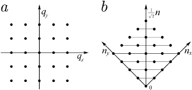
Figure 2: Cartesian eigenvalues following the asignments of position and energy generators in (4.2) within the algebra so($4$). (a): Position eigenvalues $(q_{x},q_{y})$ in (4.3). (b): sum and difference of mode eigenvalues $(n_{x},n_{y})$ in (4.4).

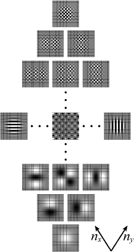
Figure 3: Basis of $x$- and $y$-mode eigenstates on the Cartesian array, $\Psi^{\lower 2.0pt\hbox{\tiny{\char 48\relax}}}_{n_{x},n_{y}}(q_{x},q_{y})$ in (4.5).

4.2 The polar coordinate system

The six generators of the Lie algebra so($4$) can be identified with positions and modes following an asignment different from the Cartesian direct sum of the previous section. We indicate the new generators with a circle super-index, $X^{\circ}_{i}$; as in the classical case, a generator of rotations $M$ between the $x$- and $y$-axes should satisfy the commutation relations

$$[M,Q^{\circ}_{x}]={\rm i}Q^{\circ}_{y},\qquad [M,Q^{\circ}_{y}]=-{\rm i}Q^{\circ}_{x},$$ (4.6)

$$[M,P^{\circ}_{x}]={\rm i}P^{\circ}_{y},\qquad [M,P^{\circ}_{y}]=-{\rm i}P^{\circ}_{x},$$ (4.7)

while the isotropic Fourier generator $K=J_{1,2}$ should rotate between position and momentum operators,

$$[K,Q^{\circ}_{x}]={\rm i}P^{\circ}_{x},\qquad [K,P^{\circ}_{x}]=-{\rm i}Q^{\circ}_{x},$$ (4.8)

$$[K,Q^{\circ}_{y}]={\rm i}P^{\circ}_{y},\qquad [K,P^{\circ}_{y}]=-{\rm i}Q^{\circ}_{y},\qquad\hbox{and}$$ (4.9)

$$[K,M]=0.$$ (4.10)

The commutator (4.10) asserts that $K$ and $M$ can be used to define a basis for ${\cal C}^{N^{2}}$ with the quantum numbers of mode and angular momentum, that will be given below. Expressed in the pattern (4.1), a new so($4$) generator assignment that fulfills these requirements is

$$\vbox{\vbox{\hbox{}\vskip-10.8pt\vbox to19.91684pt{\vss\hbox to85.35826pt{\hfil$\displaystyle\hfill\framebox{\vbox to19.91684pt{\vfil\hbox to19.91684pt{\hfil$\displaystyle K$\hfil}\vfil}}\hskip 0.0pt\hbox{}\framebox{\vbox to19.91684pt{\vfil\hbox to19.91684pt{\hfil$\displaystyle\!{-}P^{\circ}_{x}$\hfil}\vfil}}\hskip 0.0pt\hbox{}\framebox{\vbox to19.91684pt{\vfil\hbox to19.91684pt{\hfil$\displaystyle\!{-}P^{\circ}_{y}$\hfil}\vfil}}\hskip 0.0pt\hbox{}$\hfil}\vss}\vskip-11.8pt\hbox{} \hbox{}\vskip-10.8pt\vbox to19.91684pt{\vss\hbox to85.35826pt{\hfil$\displaystyle\hfill\framebox{\vbox to19.91684pt{\vfil\hbox to19.91684pt{\hfil$\displaystyle Q^{\circ}_{x}$\hfil}\vfil}}\hskip 0.0pt\hbox{}\framebox{\vbox to19.91684pt{\vfil\hbox to19.91684pt{\hfil$\displaystyle Q^{\circ}_{y}$\hfil}\vfil}}\hskip 0.0pt\hbox{}$\hfil}\vss}\vskip-11.8pt\hbox{} \hbox{}\vskip-10.8pt\vbox to19.91684pt{\vss\hbox to85.35826pt{\hfil$\displaystyle\hfill\framebox{\vbox to19.91684pt{\vfil\hbox to19.91684pt{\hfil$\displaystyle M$\hfil}\vfil}}\hskip 0.0pt\hbox{}$\hfil}\vss}\vskip-11.8pt\hbox{}}}\;.$$ (4.11)

This assignment satisfies the conditions (4.6)–(4.10), but implies the further commutators

$$[Q^{\circ}_{x},P^{\circ}_{x}]={\rm i}K=[Q^{\circ}_{y},P^{\circ}_{y}],$$ (4.12)

$$[Q^{\circ}_{x},Q^{\circ}_{y}]={\rm i}M=[P^{\circ}_{x},P^{\circ}_{y}],$$ (4.13)

$$[Q^{\circ}_{x},P^{\circ}_{y}]=0=[Q^{\circ}_{y},P^{\circ}_{x}].$$

Of these, (4.12) echoes the su($2$) nonstandard commutator in (3.4), while the commutator (4.13) is also nonstandard, and indicates that $Q^{\circ}_{x}$ and $Q^{\circ}_{y}$ cannot be simultaneously diagonalized.

First, we find operators with quantum numbers corresponding to radius and angle; we use the subalgebra chain

$$K \!{-}P^{\circ}_{x} \!{-}P^{\circ}_{y} Q^{\circ}_{x} Q^{\circ}_{y} M \supset Q^{\circ}_{x} Q^{\circ}_{y} M \supset M$$         (4.14)

When both su($2$)’s in (4.2) have the same Casimir eigenvalue $j(j+1)$, the principal Casimir invariant is $\sum\limits_{i<i^{\prime}}J_{i,i^{\prime}}^{2}=2j(j+1)1$. In so($4$) there is a second invariant, $\sum\limits_{(i<i^{\prime})\neq(k<k^{\prime})}J_{i,i^{\prime}}J_{k,k^{\prime}}$, which is identically zero in these ‘square’ cases [23]. Let us now consider the Casimir operator of the subalgebra $\hbox{\sf so($3$)}\subset\hbox{\sf so($4$)}$ in (4.14), which is

$$R(R+1):=(Q^{\circ}_{x})^{2}+(Q^{\circ}_{y})^{2}+M^{2}.$$ (4.15)

The Gel’fand–Tsetlin branching rules [26] determine that ${\cal C}^{N^{2}}$ then decomposes into subspaces ${\cal C}^{\rho}$ that are irreducible under this so($3$), where (4.15) exhibits the eigenvalues [23]

$$\rho(\rho+1),\qquad\rho\in\{0,1,\ldots,j-1\}.$$

Although $R$ is not an element of the algebra so($4$), we shall identify it as the radius operator. The final link in the reduction (4.14) is $M$, whose eigenvalues in the $\rho$-representation of so($3$) are $m\in\{-\rho,-\rho+1,\ldots,\rho\}$. The total number of distinct eigenvalue pairs $(\rho,m)$ is $\sum\limits_{\rho=0}^{2j}(2\rho+1)=(2j+1)^{2}=N^{2}$, the same as for the $N\times N$ square grid, and shown in Fig. 4a. Thus we define the radius-angular momentum (ra) eigenvectors

$$R\,|\rho,m\rangle_{\!{\scriptscriptstyle\rm RA}}^{\circ}=\rho\,|\rho,m\rangle_{\!{\scriptscriptstyle\rm RA}}^{\circ},\qquad M\,|\rho,m\rangle_{\!{\scriptscriptstyle\rm RA}}^{\circ}=m\,|\rho,m\rangle_{\!{\scriptscriptstyle\rm RA}}^{\circ},\qquad\rho|_{0}^{2j},\qquad m|_{-\rho}^{\rho},$$ (4.16)

and we adopt $\rho$ as the radial position coordinate.

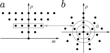
Figure 4: Polar eigenvalues following the asignments of radius and angle in (4.17) within the algebra reduction $\hbox{\sf so($4$)}\supset\hbox{\sf so($3$)}\supset\hbox{\sf so($2$)}$ in (4.14). Left: Eigenvalues $(\rho,m)$ in (4.16). Right: Positions of radius $\rho$ and angles $\phi_{k}$ according to (4.17) aligned by $\psi_{\rho}=0$.

In the last step we use the discrete Fourier transform matrix, ${\bf F}_{\rho}$ in each $(2\rho+1)$-dimensional subspace, to pass between angular momenta and angles, and thus build the Kronecker basis of states $\,|\rho,\phi\rangle_{\!{\scriptscriptstyle\rm\odot}}$ localized at a definite radius $\rho$ and the $2\rho+1$ equidistant angles $\phi_{k}$ as

$$\,|\rho,\phi_{k}\rangle_{\!{\scriptscriptstyle\rm\odot}}:=\frac{1}{\surd 2\rho+1}\sum_{m=-\rho}^{\rho}\exp(-{\rm i}m\phi_{k})\,\,|\rho,m\rangle_{\!{\scriptscriptstyle\rm RA}}^{\circ},$$ (4.17)

$$\,|\rho,m\rangle_{\!{\scriptscriptstyle\rm RA}}^{\circ}=\frac{1}{\surd 2\rho+1}\sum_{k=-\rho}^{\rho}\exp(+{\rm i}m\phi_{k})\,\,|\rho,\phi_{k}\rangle_{\!{\scriptscriptstyle\rm\odot}}$$

$$\hbox{for}\quad\phi_{k}:=2\pi k/(2\rho+1)+\psi_{\rho},\qquad-\rho\leq k\leq\rho,$$

where the $\psi_{\rho}$’s are fixed but arbitrary phases. In Fig. 4b we show the resulting arrangement of $N^{2}$ points $(\rho,\phi_{k})$ thus defined. Note that the Fourier transformation in (4.17) is linear and unitary but is not an element of the group SO($4$): it has been imported to act on each of the $2\rho+1$-dimensional so($3$) irreducible representation subspaces $\rho\in\{0,1,\ldots,2j\}$.

Having the position Kronecker eigenstate basis $\,|\rho,\phi_{k}\rangle_{\!{\scriptscriptstyle\rm\odot}}$ for polar coordinates, we now define the basis of mode and angular momentum ma, eigenbasis of the commuting operators $K=K^{{\lower 2.0pt\hbox{\tiny{\char 48\relax}}}}_{x}+K^{{\lower 2.0pt\hbox{\tiny{\char 48\relax}}}}_{y}$ with total mode number $n|_{0}^{4j}$ (pseudo-energy $\kappa=n-2j$), and of $M=K^{{\lower 2.0pt\hbox{\tiny{\char 48\relax}}}}_{x}+K^{{\lower 2.0pt\hbox{\tiny{\char 48\relax}}}}_{y}$ with angular momentum $m$, placed in the pattern (4.11). We build these eigenstates $\,|n,m\rangle_{\!{\scriptscriptstyle\rm MA}}^{\circ}$ asking for

$$K\,|n,m\rangle_{\!{\scriptscriptstyle\rm MA}}^{\circ}=(n-2j)\,|n,m\rangle_{\!{\scriptscriptstyle\rm MA}}^{\circ},\qquad M\,|n,m\rangle_{\!{\scriptscriptstyle\rm MA}}^{\circ}=m\,|n,m\rangle_{\!{\scriptscriptstyle\rm MA}}^{\circ}.$$ (4.18)

We observe that whereas the ra states in (4.16) are classified by the Gel’fand–Tsetlin chain of subalgebras $\hbox{\sf so($4$)}\supset\hbox{\sf so($3$)}\supset\hbox{\sf so($2$)}$, the ma states in (4.18) follow the chain $\hbox{\sf so($4$)}=\hbox{\sf su($2$)}\oplus\hbox{\sf su($2$)}\supset\hbox{\sf u($1$)}\oplus\hbox{\sf u($1$)}$, which in ordinary quantum theory entails the coupling of two spin-$j$ representations to total spin $\rho$. The overlaps between the ma and ra states should therefore be Clebsch–Gordan coefficients $\sim C\phantom{|}^{j\,,}_{m_{1},}\phantom{|}{}^{j\,,}_{m_{2},}\phantom{|}{}^{j}_{m}$, with $m_{1}=\textstyle\frac{1}{2}(\kappa+m)$ and $m_{2}=-\textstyle\frac{1}{2}(\kappa-m)$, adding to the total $m$ [23]. In the present construction though, the subalgebra chain (4.14) reduces along the ‘lower’ subalgebras, and this differs from the original Gel’fand–Tsetlin reduction that reduces along the upper ones; also, generally one counts su($2$) multiplet states from the top down, and we have ordered them from the bottom up. The overlap of ra and ma states entails an extra phase that must be computed carefully. It is [19, 20]

$$\!\!\!\!\phantom{{|}e}{}_{{\scriptscriptstyle\rm RA}}^{{}\!\!{}\ \ \,\circ}\!\langle{\rho,m}|{\kappa+j,m}\rangle_{{\scriptscriptstyle\rm MA}}^{\circ}=\varphi(j,\rho,\kappa,m)\,C\phantom{|}^{j\,,}_{(m+\kappa)/2,}\phantom{|}{}^{j\,,}_{(m-\kappa)/2,}\phantom{|}{}^{\rho}_{m\mathstrut},$$

$$\varphi(j,\rho,\kappa,m):=(-1)^{j+\rho}\exp[{\rm i}\textstyle\frac{1}{2}\pi(\kappa+|m|-m)].$$

The overlap between the states of mode $n=\kappa+j$ and angular momentum $m$ with the polar Kronecker basis of radius $\rho$ and angle $\phi_{k}$ yields the discrete polar oscillator wavefunctions

$$\Psi^{\circ}_{n,m}(\rho,\phi_{k}):=\!\!\!\!\phantom{{|}e}_{{\scriptscriptstyle\rm\odot}}^{{}\!\!}\!\langle{\rho,\phi_{k}}|{n-j,m}\rangle_{{\scriptscriptstyle\rm MA}}^{\circ}$$

$$\phantom{\Psi^{\circ}_{n,m}(\rho,\phi_{k})}{}\,=\frac{1}{\sqrt{2\rho+1}}\sum_{m=-\rho}^{\rho}e^{{\rm i}m\phi_{k}}\varphi(j,\rho,\kappa,m)\,C\phantom{|}^{j\,,}_{(m+n-j)/2,}\phantom{|}{}^{j\,,}_{(m-n+j)/2,}\phantom{|}{}^{\rho}_{m\mathstrut}.$$ (4.19)

These states are accommodated in a rhombus $(n,m)$, similar but distinct from the rhombus in Fig. 2, which was classified by $(n_{x},n_{y})$; here it consists of the eigenvalue pairs

$$n|_{0}^{2j},\qquad m\in\{-n,-n+2,\ldots,n\},$$

$$n|_{2j}^{4j},\qquad m\in\{-4j+n,-4j+n+2,\ldots,4j-n\}.$$ (4.20)

In Fig. 5 we show the ${\cal C}^{N^{2}}$ basis of ma states. Note that due to the Clebsch–Gordan selection rules, states of a given angular momentum $m$ are nonzero only at radii $\rho\geq|m|$.

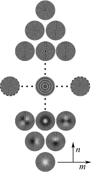
Figure 5: Basis of mode-angular momentum eigenstates on the polar array of radius and angle, $\Psi^{\circ}_{n,m}(\rho,\phi_{k})$ in (4.19).

The generator $K$ in (4.11) generates rotations between both position and momentum operators, and corresponds to twice the isotropic Fourier transform generator $2\bar{F}_{0}$ in (2.3). The action of ${\cal K}(\omega):=\exp(-{\rm i}\omega K)$ on the ma basis of ${\cal C}^{N^{2}}$ is thus

$${\cal K}(\omega)\,\,|n,m\rangle_{\!{\scriptscriptstyle\rm MA}}^{\circ}=e^{-2{\rm i}(n-2j)\omega}\,\,|n,m\rangle_{\!{\scriptscriptstyle\rm MA}}^{\circ}.$$ (4.21)

Similarly, rotations are generated by angular momentum, ${\cal R}(\theta):=\exp(-{\rm i}\theta M)$; and since $M$ is twice the generator $\bar{F}_{3}\in\hbox{\sf SU($2$)}_{\scriptscriptstyle\rm F}$ in (2.6), the vectors in the polar basis (4.19) of ${\cal C}^{N^{2}}$ are multiplied by a phase with the double angle,

$${\cal R}(\theta)\,\,|n,m\rangle_{\!{\scriptscriptstyle\rm MA}}^{\circ}=e^{-2{\rm i}m\theta}\,\,|n,m\rangle_{\!{\scriptscriptstyle\rm MA}}^{\circ}.$$ (4.22)

Under these rotations, images $f(\rho,\phi_{k})=\phantom{{|}}_{{\scriptscriptstyle\rm\odot}}^{{}\!\!}\!\langle{\rho,\phi_{k}}|\,f\,\rangle$ on the polar-pixellated screen will thus transform into

$$f_{\theta}(\rho,\phi_{k}):=f(\rho,\phi_{k}+\theta)=\phantom{{|}}_{{\scriptscriptstyle\rm\odot}}^{{}\!\!}\!\langle{\rho,\phi_{k}}|{\cal R}(\theta)\,|\,f\rangle$$

$$\phantom{f_{\theta}(\rho,\phi_{k})}{}\,=\phantom{{|}}_{{\scriptscriptstyle\rm\odot}}^{{}\!\!}\!\langle{\rho,\phi_{k}}|\exp(-{\rm i}\theta M)\,|\rho,m\rangle_{\!{\scriptscriptstyle\rm RA}}^{\circ}\phantom{{|}}{}_{{\scriptscriptstyle\rm RA}}^{{}\!\!{}\ \circ}\!\langle{\rho,m}|f\rangle$$

$$\phantom{f_{\theta}(\rho,\phi_{k})}{}\,=\sum_{k^{\prime}=-\rho}^{\rho}R^{\circ}(\rho;\phi_{k},\phi_{k^{\prime}};\theta)f(\rho,\phi_{k^{\prime}})=f(\rho,\phi_{k}-\theta),$$

where for each radius $\rho|_{0}^{2j}$ there is a $(2\rho+1)\times(2\rho+1)$ matrix representing the same rotation

$$R^{\circ}(\rho;\phi_{k},\phi_{k^{\prime}};\theta):=\!\!\!\!\phantom{{|}e}_{{\scriptscriptstyle\rm\odot}}^{{}\!\!}\!\langle{\rho,\phi_{k}}|{\rho,m}\rangle_{{\scriptscriptstyle\rm RA}}^{\circ}\exp(-{\rm i}\theta m)\!\!\!\phantom{{|}e}_{{\scriptscriptstyle\rm RA}}^{{}\!\!{}\ \circ}\!\langle{\rho,m}|{\rho,\phi_{k^{\prime}}}\rangle_{{\scriptscriptstyle\rm\odot}}$$

$$\phantom{R^{\circ}(\rho;\phi_{k},\phi_{k^{\prime}};\theta)}{}\,=\frac{1}{2\rho+1}\sum_{m=-\rho}^{\rho}\exp[-{\rm i}m(\theta-\phi_{k}+\phi_{k^{\prime}})]$$

$$\phantom{R^{\circ}(\rho;\phi_{k},\phi_{k^{\prime}};\theta)}{}\,=\frac{1}{2\rho+1}\frac{\sin[(\rho+\textstyle\frac{1}{2})(\theta-\phi_{k}+\phi_{k^{\prime}})]}{\sin\textstyle\frac{1}{2}(\theta-\phi_{k}+\phi_{k^{\prime}})}.$$ (4.23)

These are circulating matrices, functions of $\phi_{k}-\phi_{k^{\prime}}=2\pi(k-k^{\prime})/(2\rho+1)$ modulo $2\pi$, and periodic in $k$, $k^{\prime}$ modulo $2\rho+1$. For each radius, the ‘unit’ rotation angle is $\theta=2\pi/(2\rho+1)$, and for multiples $l$ thereof, the matrix (4.23) is nonzero at the diagonal $k=k^{\prime}+l$. In Fig. 6 we give an example of such rotation.

Figure 6: Rotation of images on the polar screen.

Isotropic Fourier transformations and rotations on the polar screen are produced by generators within the so($4$) algebra in the pattern (4.11). However, the pattern also informs us that with linear combinations of $K$ and $M$, we can not gyrate the planes $(Q^{\circ}_{x},P^{\circ}_{y})$ and $(Q^{\circ}_{y},P^{\circ}_{x})$ jointly as with $2\bar{F}_{2}$ in (2.5); also missing is the anisotropic Fourier transform generated by $2\bar{F}_{1}$ in (2.4), which was natural in the Cartesian basis. These transformations will be imported on ${\cal C}^{N^{2}}$ in Section 7.

5 Importation of rotations on the Cartesian screen

We noted above that in the subalgebra chain (4.14), the generators of isotropic Fourier transformations and rotations, $K\leftrightarrow 2\bar{F}_{0}$ and $M\leftrightarrow 2\bar{F}_{3}$ are domestic to so($4$), while anisotropic Fourier transformations and gyrations, corresponding to $2\bar{F}_{2}$, are foreign. Now, in the Cartesian subalgebra decomposition of so($4$) in (4.2), the two independent Fourier transform generators (2.3), (2.4), $K^{{\lower 2.0pt\hbox{\tiny{\char 48\relax}}}}_{x}\leftrightarrow\bar{F}_{0}+\bar{F}_{1}$ and $K^{{\lower 2.0pt\hbox{\tiny{\char 48\relax}}}}_{y}\leftrightarrow\bar{F}_{0}-\bar{F}_{1}$ are domestic to so($4$), while those of gyrations and rotations, $2\bar{F}_{2}$ and $2\bar{F}_{3}$, are foreign. Since we cannot complete a fully domestic $\hbox{\sf U($2$)}_{\scriptscriptstyle\rm K}$ Fourier–Kravchuk group in correspondence with the Fourier group $\hbox{\sf U($2$)}_{\scriptscriptstyle\rm F}\subset\hbox{\sf Sp($4,\Re$)}$, we must import the missing transformations. Such importation was used in (4.17) with the $(2\rho+1)\times(2\rho+1)$ discrete Fourier transform matrix.

We now build the group of rotations on the Cartesian grid by importing SU($2$) transformations [23, Chapter 3] from the continuous model. Rotations of an image should respect the energy of each formant mode $n=n_{x}+n_{y}=\kappa+2j$ in the $\,|n_{x},n_{y}\rangle_{\!{\scriptscriptstyle\rm 3}}^{{\lower 2.0pt\hbox{\tiny{\char 48\relax}}}}$ basis of ${\cal C}^{N^{2}}$, and transforms real images into real ones, while mixing states with different eigenvalues $\mu:=\textstyle\frac{1}{2}(n_{x}-n_{y})$, $\mu|_{-n/2}^{n/2}$, horizontally across the rhombus in Fig. 2b. The proposed imported action of $\bar{F}_{3}$ in (2.6) on the Cartesian modes stems from (3.3), replacing $j\mapsto\textstyle\frac{1}{2}(n_{x}+n_{y})=\textstyle\frac{1}{2}n$ and $m\equiv\mu\mapsto\textstyle\frac{1}{2}(n_{x}-n_{y})$, namely

$$M\,|n_{x},n_{y}\rangle_{\!{\scriptscriptstyle\rm 3}}^{{\lower 2.0pt\hbox{\tiny{\char 48\relax}}}}=\sqrt{n_{y}(n_{x}+1)}\,|n_{x}+1,n_{y}-1\rangle_{\!{\scriptscriptstyle\rm 3}}^{{\lower 2.0pt\hbox{\tiny{\char 48\relax}}}}+\sqrt{n_{x}(n_{y}+1)}\,|n_{x}-1,n_{y}+1\rangle_{\!{\scriptscriptstyle\rm 3}}^{{\lower 2.0pt\hbox{\tiny{\char 48\relax}}}}.$$ (5.1)

We must pay attention to the fact that $\bar{F}_{3}$ in (2.6) is one-half of the angular momentum operator $q_{x}p_{y}-q_{y}p_{x}$ that is the generator of finite rotations, ${\cal R}(\theta)\leftrightarrow\exp(-2{\rm i}\theta\bar{F}_{3})$. On the Cartesian mode basis states its action involves the standard Wigner little-$d$ function (3.8) through

$${\cal R}(\theta)\,|n_{x},n_{y}\rangle_{\!{\scriptscriptstyle\rm 3}}^{{\lower 2.0pt\hbox{\tiny{\char 48\relax}}}}=\sum_{n^{\prime}_{x}+n^{\prime}_{y}=n}d^{n/2}_{(n_{x}-n_{y})/2,(n^{\prime}_{x}-n^{\prime}_{y})/2}(2\theta)\,|n^{\prime}_{x},n^{\prime}_{y}\rangle_{\!{\scriptscriptstyle\rm 3}}^{{\lower 2.0pt\hbox{\tiny{\char 48\relax}}}}.$$

This is a real linear combination of the Cartesian mode basis where $n$ and $\mu$ are bound within the rhombus of Fig. 2b, for integer $n|_{0}^{2j}$, $\mu|_{-n/2}^{n/2}$ in the lower half and for $n|_{2j}^{4j}$, $\mu|_{n/2-j}^{2j-n/2}$ in the upper one.

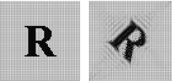
Figure 7: Rotation of images on the square screen.

In Fig. 7 we show rotation of a Cartesian-pixellated image $f(q_{x},q_{y})=\phantom{{|}}_{{\scriptscriptstyle\rm 1}}^{{}\!\!}\!\langle{q_{x},q_{y}}|f\rangle$ to

$$f_{\theta}(q_{x},q_{y}):=\phantom{{|}}_{{\scriptscriptstyle\rm 1}}^{{}\!\!{\lower 2.0pt\hbox{\tiny{\char 48\relax}}}}\!\langle{q_{x},q_{y}}|{\cal R}(\theta)\,|f\rangle=\phantom{{|}}_{{\scriptscriptstyle\rm 1}}^{{}\!\!{\lower 2.0pt\hbox{\tiny{\char 48\relax}}}}\!\langle{q_{x},q_{y}}|{\cal R}(\theta)\,\,|n_{x},n_{y}\rangle_{\!{\scriptscriptstyle\rm 3}}^{{\lower 2.0pt\hbox{\tiny{\char 48\relax}}}}\phantom{{|}e}{}_{{\scriptscriptstyle\rm 3}}^{{}\!\!{\lower 2.0pt\hbox{\tiny{\char 48\relax}}}}\!\langle{n_{x},n_{y}}|{q^{\prime}_{x},q^{\prime}_{y}}\rangle_{{\scriptscriptstyle\rm 1}}^{{\lower 2.0pt\hbox{\tiny{\char 48\relax}}}}\phantom{{|}}{}_{{\scriptscriptstyle\rm 1}}^{{}\!\!{\lower 2.0pt\hbox{\tiny{\char 48\relax}}}}\!\langle{q^{\prime}_{x},q^{\prime}_{y}}|f\rangle$$

$$\phantom{f_{\theta}(q_{x},q_{y})}{}\,=\sum_{q^{\prime}_{x},q^{\prime}_{y}}R^{{\lower 2.0pt\hbox{\tiny{\char 48\relax}}}}(q_{x},q_{y};q^{\prime}_{x},q^{\prime}_{y};\theta)f(q^{\prime}_{x},q^{\prime}_{y}).$$

The subgroup of rotations ${\cal R}(\theta)\in\hbox{\sf SU($2$)}_{\scriptscriptstyle\rm K}$ is thus represented by the $N^{2}\times N^{2}$ matrices

$$R^{\lower 2.0pt\hbox{\tiny{\char 48\relax}}}(q_{x},q_{y};q^{\prime}_{x},q^{\prime}_{y};\theta):=\!\!\!\phantom{{|}e}_{{\scriptscriptstyle\rm 1}}^{{}\!\!{\lower 2.0pt\hbox{\tiny{\char 48\relax}}}}\!\langle{q_{x},q_{y}}|{n_{x},n_{y}}\rangle_{{\scriptscriptstyle\rm 3}}^{{\lower 2.0pt\hbox{\tiny{\char 48\relax}}}}\phantom{{|}}{}_{{\scriptscriptstyle\rm 3}}^{{}\!\!{\lower 2.0pt\hbox{\tiny{\char 48\relax}}}}\!\langle{n_{x},n_{y}}|{\cal R}(\theta)\,|n^{\prime}_{x},n^{\prime}_{y}\rangle_{\!{\scriptscriptstyle\rm 3}}^{{\lower 2.0pt\hbox{\tiny{\char 48\relax}}}}\!\!\phantom{{|}e}{}_{{\scriptscriptstyle\rm 3}}^{{}\!\!{\lower 2.0pt\hbox{\tiny{\char 48\relax}}}}\!\langle{n^{\prime}_{x},n^{\prime}_{y}}|{q^{\prime}_{x},q^{\prime}_{y}}\rangle_{{\scriptscriptstyle\rm 1}}^{{\lower 2.0pt\hbox{\tiny{\char 48\relax}}}}$$

$$\phantom{R^{\lower 2.0pt\hbox{\tiny{\char 48\relax}}}(q_{x},q_{y};q^{\prime}_{x},q^{\prime}_{y};\theta)}{}\,=\sum_{\mu,\mu^{\prime}}\Psi^{\lower 2.0pt\hbox{\tiny{\char 48\relax}}}_{n_{x},n_{y}}(q_{x},q_{y})d^{n/2}_{\mu,\mu^{\prime}}(2\theta)\Psi^{\lower 2.0pt\hbox{\tiny{\char 48\relax}}}_{n^{\prime}_{x},n^{\prime}_{y}}(q^{\prime}_{x},q^{\prime}_{y}),$$ (5.2)

where $\mu=\textstyle\frac{1}{2}(n_{x}-n_{y})$ and $\mu^{\prime}=\textstyle\frac{1}{2}(n^{\prime}_{x}-n^{\prime}_{y})$ are bound by $n_{x}+n_{y}=n=n^{\prime}_{x}+n^{\prime}_{y}$, and belong to the same row in the rhombus of Fig. 2b.

6 Completion of $\boldsymbol{\hbox{\sf U($2$)}_{\scriptscriptstyle\rm K}}$ on the Cartesian screen

Having imported a unitary representation of the group of rotations onto pixellated images on the Cartesian screen, and having the domestic group of fractional Fourier transforms, we can complete the Fourier–Kravchuk group $\hbox{\sf U($2$)}_{\scriptscriptstyle\rm K}$ on this screen. From (2.4) and (4.2), $\bar{F}_{1}\leftrightarrow\textstyle\frac{1}{2}(K^{\lower 2.0pt\hbox{\tiny{\char 48\relax}}}_{x}-K^{\lower 2.0pt\hbox{\tiny{\char 48\relax}}}_{y})$, the Lie exponential ${\cal A}(\phi)\leftrightarrow\exp(-2{\rm i}\phi\bar{F}_{1})$ acts on the Cartesian kets (4.4) through phases,

$${\cal A}(\phi)\,|n_{x},n_{y}\rangle_{\!{\scriptscriptstyle\rm 1}}^{{\lower 2.0pt\hbox{\tiny{\char 48\relax}}}}=\exp[-2{\rm i}\phi(n_{x}-n_{y})]\,|n_{x},n_{y}\rangle_{\!{\scriptscriptstyle\rm 1}}^{{\lower 2.0pt\hbox{\tiny{\char 48\relax}}}}.$$ (6.1)

Hence, for images $f(q_{x},q_{y})$,

$$f_{\phi}(q_{x},q_{y}):={\cal A}(\phi)\,f(q_{x},q_{y})=\sum_{q^{\prime}_{x},q^{\prime}_{y}}A^{\lower 2.0pt\hbox{\tiny{\char 48\relax}}}(q_{x},q_{y};q^{\prime}_{x},q^{\prime}_{y};\phi)f(q^{\prime}_{x},q^{\prime}_{y}),$$

with the matrix kernel

$$A^{\lower 2.0pt\hbox{\tiny{\char 48\relax}}}(q_{x},q_{y};q^{\prime}_{x},q^{\prime}_{y};\phi)=\sum_{\mu}\Psi^{\lower 2.0pt\hbox{\tiny{\char 48\relax}}}_{n_{x},n_{y}}(q_{x},q_{y})\exp[-2{\rm i}\phi(n_{x}-n_{y})]\Psi^{\lower 2.0pt\hbox{\tiny{\char 48\relax}}}_{n_{x},n_{y}}(q^{\prime}_{x},q^{\prime}_{y}),$$ (6.2)

where the sum over $\mu=\textstyle\frac{1}{2}(n_{x}-n_{y})$ preserves $n$.

Now, having two of the three generators of $\hbox{\sf SU($2$)}_{\scriptscriptstyle\rm K}$, we can produce the third: gyrations ${\cal G}(\psi)\leftrightarrow\exp(-2{\rm i}\psi\bar{F}_{2})$, through

$${\cal G}(\psi)={\cal A}({\textstyle\frac{1}{4}}\pi){\cal R}(\psi){\cal A}({\textstyle\frac{1}{4}}\pi)^{-1}.$$

On images $f(q_{x},q_{y})$, Fourier–Kravchuk gyrations will act through a matrix kernel,

$$f_{\psi}(q_{x},q_{y}):={\cal G}(\psi)\,f(q_{x},q_{y})=\sum_{q^{\prime}_{x},q^{\prime}_{y}}G^{\lower 2.0pt\hbox{\tiny{\char 48\relax}}}(q_{x},q_{y};q^{\prime}_{x},q^{\prime}_{y};\psi)f(q^{\prime}_{x},q^{\prime}_{y}),$$

$$G^{\lower 2.0pt\hbox{\tiny{\char 48\relax}}}(q_{x},q_{y};q^{\prime}_{x},q^{\prime}_{y};\psi)=\sum_{\mu,\mu^{\prime}}\Psi^{\lower 2.0pt\hbox{\tiny{\char 48\relax}}}_{n_{x},n_{y}}(q_{x},q_{y})e^{-{\rm i}\pi\mu/4}\,d^{n/2}_{\mu,\mu^{\prime}}(2\psi)e^{+{\rm i}\pi\mu^{\prime}/4}\Psi^{\lower 2.0pt\hbox{\tiny{\char 48\relax}}}_{n^{\prime}_{x},n^{\prime}_{y}}(q^{\prime}_{x},q^{\prime}_{y}),$$

where, as in (5.2) and (6.2), the sums over $\mu=\textstyle\frac{1}{2}(n_{x}-n_{y})$ and $\mu^{\prime}=\textstyle\frac{1}{2}(n^{\prime}_{x}-n^{\prime}_{y})$ preserve $n$. In continuum optics, gyrations acting on the Hermite–Gauss beams transform them into Laguerre–Gauss ones of the same mode number [22, Fig. 4].

Finally, the isotropic ${\cal K}(\omega)\leftrightarrow\exp(-2{\rm i}\omega\bar{F}_{0})$ in (4.21) is domestic to the so($4$) algebra (4.2), and completes the $\hbox{\sf U($2$)}_{\scriptscriptstyle\rm K}$ group with

$$f_{\omega}(q_{x},q_{y}):={\cal K}(\omega)\,f(q_{x},q_{y})=\sum_{q^{\prime}_{x},q^{\prime}_{y}}K^{\lower 2.0pt\hbox{\tiny{\char 48\relax}}}(q_{x},q_{y};q^{\prime}_{x},q^{\prime}_{y};\omega)f(q^{\prime}_{x},q^{\prime}_{y}),$$

$$K^{\lower 2.0pt\hbox{\tiny{\char 48\relax}}}(q_{x},q_{y};q^{\prime}_{x},q^{\prime}_{y};\omega)=\sum_{n_{x},n_{y}}\Psi^{\lower 2.0pt\hbox{\tiny{\char 48\relax}}}_{n_{x},n_{y}}(q_{x},q_{y})\,\exp[-2{\rm i}\omega(n_{x}+n_{y})]\Psi^{\lower 2.0pt\hbox{\tiny{\char 48\relax}}}_{n_{x},n_{y}}(q^{\prime}_{x},q^{\prime}_{y}).$$

The elements of the Fourier group $\hbox{\sf U($2$)}_{\scriptscriptstyle\rm F}=\hbox{\sf U($1$)}_{\scriptscriptstyle\rm F}\otimes\hbox{\sf SU($2$)}_{\scriptscriptstyle\rm F}$, where the factors are complementary, are customarily parametrized by Euler angles as

$$\bar{\cal D}(\omega;\phi,\theta,\psi):=\exp(-{\rm i}\omega\bar{F}_{0})\exp(-{\rm i}\phi\bar{F}_{3})\exp(-{\rm i}\theta\bar{F}_{2})\exp(-{\rm i}\psi\bar{F}_{3}),$$ (6.3)

and its matrix elements between eigenstates $\phantom{{|}}{}^{{}\!\!}\!\langle{\iota,\mu}|$ and $\,|\iota,\mu^{\prime}\rangle_{\!{\scriptscriptstyle\rm}}$, with eigenvalues $\mu$, $\mu^{\prime}$ under $\bar{F}_{3}$ and $\iota$ under $\bar{F}_{0}$, the latter being the irreducible representation label are the well-known Wigner Big-D functions

$$D^{\iota}_{\mu,\mu^{\prime}}(\omega;\phi,\theta,\psi)=e^{-{\rm i}\iota\omega}e^{-{\rm i}\mu\phi}d^{\iota}_{\mu,\mu^{\prime}}(\theta)e^{-{\rm i}\mu^{\prime}\psi}.$$

As we indicated in Section 3, by permuting $1\mapsto 2\mapsto 3\mapsto 1$ in (6.3) and using (4.21), (4.22), and (6.1), we can write the elements of the isomorphic Fourier–Kravchuk group $\hbox{\sf U($2$)}_{\scriptscriptstyle\rm K}$ as a product of Fourier–Kravchuk transforms and rotations,

$${\cal D}(\omega;\phi,\theta,\psi)={\cal K}(\textstyle\frac{1}{2}\omega){\cal A}(\textstyle\frac{1}{2}\phi){\cal R}(\textstyle\frac{1}{2}\theta){\cal A}(\textstyle\frac{1}{2}\psi).$$

Its matrix elements between the Cartesian mode eigenstates $\,|n_{x},n_{y}\rangle_{\!{\scriptscriptstyle\rm 1}}^{{\lower 2.0pt\hbox{\tiny{\char 48\relax}}}}$ of $K^{{\lower 2.0pt\hbox{\tiny{\char 48\relax}}}}_{x}$ and $K^{{\lower 2.0pt\hbox{\tiny{\char 48\relax}}}}_{y}$will be thus,

$$\phantom{{|}}{}_{{\scriptscriptstyle\rm 1}}^{{}\!\!{\lower 2.0pt\hbox{\tiny{\char 48\relax}}}}\!\langle{n_{x},n_{y}}|{\cal D}(\omega;\phi,\theta,\psi)\,|n^{\prime}_{x},n^{\prime}_{y}\rangle_{\!{\scriptscriptstyle\rm 1}}^{{\lower 2.0pt\hbox{\tiny{\char 48\relax}}}}=e^{-{\rm i}(n-2j)\omega}D^{n/2}_{(n_{x}-n_{y})/2,(n^{\prime}_{x}-n^{\prime}_{y})/2}(\phi,\theta,\psi),$$ (6.4)

with the total mode $n=n_{x}+n_{y}=n^{\prime}_{x}+n^{\prime}_{y}$ as before.

The domestic and imported transformations properly mesh, and we see that the Fourier–Kravchuk group $\hbox{\sf U($2$)}_{\scriptscriptstyle\rm K}$ is indeed represented unitarily and faithfully by (6.4) on ${\cal C}^{N^{2}}$. Its action on images $f(q_{x},q_{y})$ pixellated on the Cartesian screen can be found from here, writing $\Omega:=(\phi,\theta,\psi)$, through a real similarity transformation by the matrix formed with the ${\cal C}^{N^{2}}$ basis (4.5) of Cartesian mode Kravchuk functions,

$$f_{\omega,\Omega}(q_{x},q_{y}):={\cal D}(\omega,\Omega)\,f(q_{x},q_{y})=\sum_{q^{\prime}_{x},q^{\prime}_{y}}D^{\lower 2.0pt\hbox{\tiny{\char 48\relax}}}(q_{x},q_{y};q^{\prime}_{x},q^{\prime}_{y};\omega,\Omega)\,f(q^{\prime}_{x},q^{\prime}_{y}),$$ (6.5)

where, with $n=n_{x}+n_{y}=n^{\prime}_{x}+n^{\prime}_{y}$ and $n|_{0}^{4j}$ the kernel is

$$D^{\lower 2.0pt\hbox{\tiny{\char 48\relax}}}(q_{x},q_{y};q^{\prime}_{x},q^{\prime}_{y};\omega,\Omega)$$

$$\qquad{}=\sum_{\textstyle{n_{x},n_{y}\atop n^{\prime}_{x}n^{\prime}_{y}}}\Psi^{\lower 2.0pt\hbox{\tiny{\char 48\relax}}}_{n_{x},n_{y}}(q_{x},q_{y})\,e^{-{\rm i}(n-2j)\omega}\,D^{n/2}_{(n_{x}-n_{y})/2,(n^{\prime}_{x}-n^{\prime}_{y})/2}(\Omega)\Psi^{\lower 2.0pt\hbox{\tiny{\char 48\relax}}}_{n^{\prime}_{x},n^{\prime}_{y}}(q^{\prime}_{x},q^{\prime}_{y}),$$ (6.6)

and these $N^{2}\times N^{2}$ matrices are unitary representations of U($2$) on the Cartesian grid of points in Fig. 2b. With this result we now turn to the polar screen.

7 The Fourier group on polar screens

In the subalgebra chain of so($4$) that produces the polar screen (4.11), the commuting rotations and isotropic Fourier–Kravchuk transforms are domestic. To complete the Fourier–Kravchuk group $\hbox{\sf U($2$)}_{\scriptscriptstyle\rm K}$ on the polar screen, we must import either gyrations or the anisotropic transform. Since these transformations have been realized already in the Cartesian screen basis, we should find a unitary map between both screens. This transformation has been studied in [19, 20], and consists in identifying the eigenstates of mode and angular momentum in both bases; in the polar basis these are $\,|\rho,m\rangle_{\!{\scriptscriptstyle\rm RA}}^{\circ}$ in (4.16) shown in Fig. 5. In the Cartesian basis such states will be constructed now as eigenvectors of ${\cal R}(\theta)=\exp(-{\rm i}\theta M)$ with eigenvalues $e^{-{\rm i}\theta m}$, or equivalently of $\bar{F}_{3}$ with eigenvalues $\textstyle\frac{1}{2}m$, corresponding to the eigenvalues of $\textstyle\frac{1}{2}M$ in (2.6). These Cartesian states will be linear combinations, respecting total mode number $n=n_{x}+n_{y}$, of all states $\,|n_{x},n_{y}\rangle_{\!{\scriptscriptstyle\rm 1}}^{{\lower 2.0pt\hbox{\tiny{\char 48\relax}}}}$,

$$\,|n,m\rangle_{\!{\scriptscriptstyle\rm MA}}^{{\lower 2.0pt\hbox{\tiny{\char 48\relax}}}}:=\sum_{n_{x}+n_{y}=n}C^{n,m}_{n_{x},n_{y}}\,|n_{x},n_{y}\rangle_{\!{\scriptscriptstyle\rm 1}}^{{\lower 2.0pt\hbox{\tiny{\char 48\relax}}}},$$

$$M\,|n,m\rangle_{\!{\scriptscriptstyle\rm MA}}^{{\lower 2.0pt\hbox{\tiny{\char 48\relax}}}}=m\,|n,m\rangle_{\!{\scriptscriptstyle\rm MA}}^{{\lower 2.0pt\hbox{\tiny{\char 48\relax}}}},\qquad K\,|n,m\rangle_{\!{\scriptscriptstyle\rm MA}}^{{\lower 2.0pt\hbox{\tiny{\char 48\relax}}}}=\textstyle\frac{1}{2}n\,|n,m\rangle_{\!{\scriptscriptstyle\rm MA}}^{{\lower 2.0pt\hbox{\tiny{\char 48\relax}}}}.$$

From (5.1), the coefficients obey the difference equation

$$\sqrt{n_{y}(n_{x}+1)}C^{n,m}_{n_{x}+1,n_{y}-1}-\textstyle\frac{1}{2}m\,C^{n,m}_{n_{x},n_{y}}+\sqrt{n_{x}(n_{y}+1)}C^{n,m}_{n_{x}-1,n_{y}+1}=0,$$

which is the ubiquitous su($2$) three-term recursion relation of the Wigner little-$d$ functions for angle $\textstyle\frac{1}{2}\pi$ (around the 1-axis [23]), now with $j\leftrightarrow\textstyle\frac{1}{2}n=\textstyle\frac{1}{2}(n_{x}+n_{y})$ and $\textstyle\frac{1}{2}m\leftrightarrow\textstyle\frac{1}{2}(n_{x}-n_{y})$. We thus define ma states having angular momentum $m$ on the square grid as

$$\,|n,m\rangle_{\!{\scriptscriptstyle\rm MA}}^{{\lower 2.0pt\hbox{\tiny{\char 48\relax}}}}:=\sum_{n_{x}+n_{y}=n}e^{{\rm i}\pi(n_{x}-n_{y})/4}d^{n/2}_{m/2,(n_{x}-n_{y})/2}(\textstyle\frac{1}{2}\pi)\,|n_{x},n_{y}\rangle_{\!{\scriptscriptstyle\rm 1}}^{{\lower 2.0pt\hbox{\tiny{\char 48\relax}}}}.$$ (7.1)

These states can be accomodated in a rhombus $(n,m)$, exactly as in (4.20).

From (7.1) follows the definition of the Cartesian basis of mode and angular momentum ma eigenstates

$$\Lambda_{n,m}^{{\lower 2.0pt\hbox{\tiny{\char 48\relax}}}}(q_{x},q_{y}):=\phantom{{|}e}_{{\scriptscriptstyle\rm 1}}^{{}\!\!{\lower 2.0pt\hbox{\tiny{\char 48\relax}}}}\!\langle{q_{x},q_{y}}|{n,m}\rangle_{{\scriptscriptstyle\rm MA}}^{{\lower 2.0pt\hbox{\tiny{\char 48\relax}}}}$$ (7.2)

$$\phantom{\Lambda_{n,m}^{{\lower 2.0pt\hbox{\tiny{\char 48\relax}}}}(q_{x},q_{y})}{}\,=\sum_{n_{x}+n_{y}=n}e^{{\rm i}\pi(n_{x}-n_{y})/4}d^{n/2}_{m/2,(n_{x}-n_{y})/2}(\textstyle\frac{1}{2}\pi)\Psi_{n_{x},n_{y}}^{{\lower 2.0pt\hbox{\tiny{\char 48\relax}}}}(q_{x},q_{y})$$

$$\phantom{\Lambda_{n,m}^{{\lower 2.0pt\hbox{\tiny{\char 48\relax}}}}(q_{x},q_{y})}{}\,=\Lambda_{n,-m}^{{\lower 2.0pt\hbox{\tiny{\char 48\relax}}}}(q_{x},q_{y})^{*}=(-1)^{n+m}\Lambda_{n,m}^{{\lower 2.0pt\hbox{\tiny{\char 48\relax}}}}(-q_{x},-q_{y})=(-1)^{q_{x}+q_{y}}\Lambda_{4j-n,-m}^{{\lower 2.0pt\hbox{\tiny{\char 48\relax}}}}(q_{x},q_{y}).$$

This transforms the Cartesian Kravchuk functions into what we called Laguerre–Kravchuk functions in [22, Fig. 4]. The basis of states (7.2) is shown in Fig. 8, which can now be identified with the basis – also of mode and angular momentum – in Fig. 5. We can now import the equivalence between the ma bases

$$\,|n,m\rangle_{\!{\scriptscriptstyle\rm MA}}^{{\lower 2.0pt\hbox{\tiny{\char 48\relax}}}}\equiv\,|n,m\rangle_{\!{\scriptscriptstyle\rm MA}}^{\circ}.$$ (7.3)

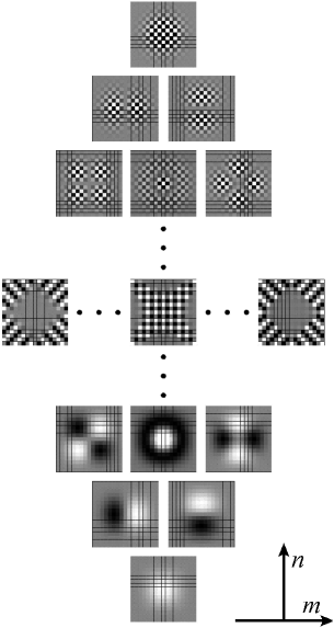
Figure 8: Basis of mode-angular momentum eigenstates on the Cartesian array, $\Lambda_{n,m}^{{\lower 2.0pt\hbox{\tiny{\char 48\relax}}}}(q_{x},q_{y})$ in (7.1).

A pixellated image on the Cartesian screen, $f_{{\lower 2.0pt\hbox{\tiny{\char 48\relax}}}}(q_{x},q_{y})\in{\cal C}^{N^{2}}$, can be thus unitarily transformed into an image on the polar screen, $f_{\circ}(\rho,\phi_{k})\in{\cal C}^{N^{2}}$ through the transformation

$$f_{\circ}(\rho,\phi_{k})=\phantom{{|}}_{{\scriptscriptstyle\rm\odot}}^{{}\!\!}\!\langle{\rho,\phi_{k}}|f\rangle$$

$$\phantom{f_{\circ}(\rho,\phi_{k})}{}=\sum_{q_{x},q_{y}}\!\!\!\phantom{{|}e}{}_{{\scriptscriptstyle\rm\odot}}^{{}\!\!}\!\langle{\rho,\phi_{k}}|{q_{x},q_{y}}\rangle_{{\scriptscriptstyle\rm 1}}^{{\lower 2.0pt\hbox{\tiny{\char 48\relax}}}}\phantom{{|}}{}_{{\scriptscriptstyle\rm 1}}^{{}\!\!{\lower 2.0pt\hbox{\tiny{\char 48\relax}}}}\!\langle{q_{x},q_{y}}|f\rangle=\sum_{q_{x},q_{y}}U(\rho,\phi_{k};q_{x},q_{y})f_{{\lower 2.0pt\hbox{\tiny{\char 48\relax}}}}(q_{x},q_{y}),$$ (7.4)

where the transform kernel, using (7.3), is

$$U(\rho,\phi_{k};q_{x},q_{y}):=\!\!\!\!\phantom{{|}e}_{{\scriptscriptstyle\rm\odot}}^{{}\!\!}\!\langle{\rho,\phi_{k}}|{q_{x},q_{y}}\rangle_{{\scriptscriptstyle\rm 1}}^{{\lower 2.0pt\hbox{\tiny{\char 48\relax}}}}$$

$$\phantom{U(\rho,\phi_{k};q_{x},q_{y})}{}\,\equiv\sum_{n,m}\!\!\!\phantom{{|}e}{}_{{\scriptscriptstyle\rm\odot}}^{{}\!\!}\!\langle{\rho,\phi_{k}}|{n,m}\rangle_{{\scriptscriptstyle\rm MA}}^{\circ}\phantom{{|}e}{}_{{\scriptscriptstyle\rm MA}}^{{}\!\!{\lower 2.0pt\hbox{\tiny{\char 48\relax}}}}\!\langle{n,m}|{q_{x},q_{y}}\rangle_{{\scriptscriptstyle\rm 1}}^{{\lower 2.0pt\hbox{\tiny{\char 48\relax}}}}=\sum_{n,m}\Psi^{\circ}_{n,m}(\rho,\phi_{k})\Lambda_{n,m}^{{\lower 2.0pt\hbox{\tiny{\char 48\relax}}}}(q_{x},q_{y})^{*}.$$

The transformation of images inverse to (7.4), from the polar to the Cartesian screen, is

$$f_{{\lower 2.0pt\hbox{\tiny{\char 48\relax}}}}(q_{x},q_{y})=\sum_{\rho,\phi_{k}}V(q_{x},q_{y};\rho,\phi_{k})f_{\circ}(\rho,\phi_{k}),$$

$$V(q_{x},q_{y};\rho,\phi_{k})=\sum_{n,m}\Lambda_{n,m}^{{\lower 2.0pt\hbox{\tiny{\char 48\relax}}}}(q_{x},q_{y})\Psi^{\circ}_{n,m}(\rho,\phi_{k})^{*}=U(\rho,\phi_{k};q_{x},q_{y})^{*}.$$

We note that these transformations map real functions onto real functions. In Fig. 9 we show an example of the map (7.4) on the 0-and-1 image of the letter R.

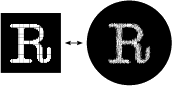
Figure 9: Unitary map (7.4) of an image (the letter R) on the Cartesian screen onto the polar screen.

The action of the Fourier–Kravchuk group $\hbox{\sf U($2$)}_{\scriptscriptstyle\rm K}$ on images on the polar screen can be now derived from its action (6.5), (6.6) on the Cartesian screen:

$$f_{\omega,\Omega}(\rho,\phi_{k}):={\cal D}(\omega,\Omega)\,f(\rho,\phi_{k})=\sum_{\rho^{\prime},\phi_{k^{\prime}}}D^{\odot}(\rho,\phi_{k};\rho^{\prime},\phi_{k^{\prime}};\omega,\Omega)f(\rho^{\prime},\phi_{k^{\prime}}),$$

where the kernel is a representation of $\hbox{\sf U($2$)}_{\scriptscriptstyle\rm K}$ on the polar screen

$$D^{\odot}(\rho,\phi_{k};\rho^{\prime},\phi_{k^{\prime}};\omega,\Omega)=\sum_{\textstyle{q_{x},q_{y}\atop q^{\prime}_{x},q^{\prime}_{y}}}U(\rho,\phi_{k};q_{x},q_{y})D^{\lower 2.0pt\hbox{\tiny{\char 48\relax}}}(q_{x},q_{y};q^{\prime}_{x},q^{\prime}_{y};\omega,\Omega)V(\rho^{\prime},\phi_{k^{\prime}};q^{\prime}_{x},q^{\prime}_{y}).$$

We have thus far not found a more compact analytic form for the representation of the Fourier group on the discrete coordinates of radius and angle.

The $N^{2}\times N^{2}$ matrix $U=(V)^{\dagger}$ that is needed above, is arduous to calculate but its numerical values need be computed only once for each size $N$ of the screen, and will serve to transform any image from the Cartesian to the polar screen and back. For $N=32$ there are $\approx 10^{6}$ values to be stored, and the transformation of an image as that in Fig. 9 between the screens involves this number of sums and products. Commercial image-rotating algorithms store the original image and interpolate the few Cartesian pixels around each geometrically determined point. Certainly, the Fourier–Kravchuk group of transformations of images presented here does not provide a fast algorithm, but it is unitary, and hence does not loose information, as interpolation invariably does; it is exact.

8 Concluding remarks

Willard Miller Jr. is recognized as having initiated the modern study of systems whose governing equation allows for separation in various coordinate systems using Lie algebraic reduction methods [27]. These equations are differential because space has been considered continuous. Finite spaces with discrete coordinates, used as foundation for finite Hamiltonian systems characterized by governing difference equations, have not been considered – to our knowledge – in the same context. The present paper reviews our work in the particular case of a two-dimensional Hamiltonian system whose two governing Hamilton equations identify as a finite harmonic oscillator, mothered by the compact algebra so($4$). And since it happens that algebra has two distinct subalgebra reductions, we can relate them with Cartesian an polar coordinates.

The difference equations whose solutions are the finite oscillator wavefunctions and the Clebsch–Gordan coefficients are contained in so($3$) and so($4$), and entail special Kravchuk and Hahn polynomials. Other finite polynomials, such as those of Meixner and Pollaczek, also appear in related harmonic oscillator models [28], and thus could be interpreted in terms of two-dimensional physical and optical models. Further, finite three-dimensional coordinate systems beyond Cartesian and circular cylindric ones may be of interest in applications. But we should end with a word of caution regarding applications: the two-dimensional arrays that purportedly measure the quality of Laguerre–Gauss (polar) laser beams generally use sampled Laguerre–Gauss functions; the question of whether these, or the mode-angular momentum finite functions, are the most efficient to find the mode and angular momenta of the actual beams, seems to favor the sampled functions [29, 30], although they do not form orthonormal bases for the space of pixellated images. But only the discrete function bases synthesize all images exactly.

The continuous two-dimensional harmonic oscillator is a superintegrable system, which is known to separate generally in elliptic coordinates, of which the Cartesian and polar are limits. We have been unable so far to find a corresponding finite array that would allow for pixellation following ellipses and hyperbolas, although there are three enticing leads: diagonalization of the so(3) operator $J^{2}+\alpha J_{3}$ [27]; a line of functions with a parameter which joins continuously Kronecker deltas with Clebsch–Gordan coefficients [31]; and the production by holographic means of laser beams whose nodes follow elliptic coordinates [32]. There are also ‘geometrical’ reasons to doubt that this is possible, however: whereas in Cartesian coordinates all pixel sizes are equal, and in polar ones they are almost so (except very near to the center), trying to visualize these two pixellations as limits of a finite elliptic pixellation presents some problems that we have not yet been able to overcome [33].

Acknowledgements

We thank the support of the Óptica Matemática projects DGAPA-UNAM IN-105008 and SEP-CONACYT 79899, and we thank Guillermo Krötzsch (ICF-UNAM) for his assistance with the graphics and Juvenal Rueda-Paz (Facultad de Ciencias, Universidad Autónoma del Estado de Morelos) for his support with the manuscript.

References

- [1]
- [2] Wolf K.B., Geometric optics on phase space, Texts and Monographs in Physics, Springer-Verlag, Berlin, 2004.
- [3] Simon R., Wolf K.B., Structure of the set of paraxial optical systems, J. Opt. Soc. Amer. A 17 (2000), 342–355.
- [4] Simon R., Wolf K.B., Fractional Fourier transforms in two dimensions, J. Opt. Soc. Amer. A 17 (2000), 2368–2381.
- [5] Moshinsky M., Quesne C., Linear canonical transformations and their unitary representation, J. Math. Phys. 12 (1971), 1772–1779.
- [6] Moshinsky M., Quesne C., Canonical transformations and matrix elements, J. Math. Phys. 12 (1971), 1780–1786.
- [7] Wolf K.B., Integral transforms in science and engineering, Mathematical Concepts and Methods in Science and Engineering, Vol. 11, Plenum Press, New York – London, 1979.
- [8] Collins S.A. Jr., Lens-system diffraction integral written in terms of matrix optics, J. Opt. Soc. Amer. A 60 (1970), 1168–1177.
- [9] Ding J.-J., Research of fractional Fourier transform and linear canonical transform, Ph.D. Thesis, National Taiwan University, 2001.
- [10] Hennelly B.M., Sheridan J.T., Fast numerical algorithm for the linear canonical transform, J. Opt. Soc. Amer. A 22 (2005), 928–937.
- [11] Koç A., Ozaktas H.M., Candan C., Kutay M.A., Digital computation of linear canonical transforms, IEEE Trans. Signal Process. 56 (2008), 2382–2394.
- [12] Healy J.J., Sheridan J.T., Sampling and discretization of the linear canonical transform, Signal Process. 89 (2009), 641–648.
- [13] Gilmore R., Lie groups, Lie algebras, and some of their applications, John Wiley, New York, 1974.
- [14] Atakishiyev N.M., Wolf K.B., Fractional Fourier–Kravchuk transform, J. Opt. Soc. Amer. A 14 (1997), 1467–1477.
- [15] Atakishiyev N.M., Vicent L.E., Wolf K.B., Continuous vs. discrete fractional Fourier transforms, J. Comput. Appl. Math. 107 (1999), 73–95.
- [16] Atakishiyev N.M., Pogosyan G.S., Vicent L.E., Wolf K.B., Finite two-dimensional oscillator. I. The Cartesian model, J. Phys. A: Math. Gen. 34 (2001), 9381–9398.
- [17] Atakishiyev N.M., Pogosyan G.S., Wolf K.B., Finite models of the oscillator, Phys. Part. Nuclei 36 (2005), 247–265.
- [18] Wolf K.B., Discrete systems and signals on phase space, Appl. Math. Inf. Sci. 4 (2010), 141–181.
- [19] Atakishiyev N.M., Pogosyan G.S., Vicent L.E., Wolf K.B., Finite two-dimensional oscillator. II. The radial model, J. Phys. A: Math. Gen. 34 (2001), 9399–9415.
- [20] Vicent L.E., Wolf K.B., Unitary transformation between Cartesian- and polar-pixellated screens, J. Opt. Soc. Amer. A 25 (2008), 1875–1884.
- [21] Vicent L.E., Unitary rotation of square-pixellated images, Appl. Math. Comput. 221 (2009), 111–117.
- [22] Wolf K.B., Alieva T., Rotation and gyration of finite two-dimensional modes, J. Opt. Soc. Amer. A 25 (2008), 365–370.
- [23] Biedenharn L.C., Louck J.D., Angular momentum in quantum mechanics, in Encyclopedia of Mathematics and its Applications, Editor G.-C. Rota, Addison-Wesley, 1981, Section 3.6.
- [24] Atakishiyev N.M., Suslov S.K., Difference analogs of the harmonic oscillator, Theoret. and Math. Phys. 85 (1991), 1055–1062.
- [25] Krawtchouk M., Sur une généralization des polinômes d’Hermite, Compt. Rend. Acad. Sci. Paris 189 (1929), 620–622.
- [26] Gel’fand I.M., Tsetlin M.L., Finite-dimensional representations of the group of unimodular matrices, Dokl. Akad. Nauk SSSR 71 (1950), 825–828 (English transl.: I.M. Gel’fand, Collected papers, Vol. II, Springer-Verlag, Berlin, 1987, 653–656).
- [27] Miller W. Jr., Symmetry and separation of variables, Encyclopedia of Mathematics and Its Applications, Vol. 4, Editor by G.-C. Rota, Addison-Wesley Publ. Co., Reading, Mass., 1981.
- [28] Atakishiyev N.M., Jafarov E.I., Nagiyev Sh.M., Wolf K.B., Meixner oscillators, Rev. Mexicana Fís. 44 (1998), 235–244.
- [29] Wolf K.B., Mode analysis and signal restoration with Kravchuk functions, J. Opt. Soc. Amer. A 26 (2009), 509–516.
- [30] Vicent L.E., Wolf K.B., Analysis of digital images into energy-angular momentum modes, J. Opt. Soc. Amer. A 28 (2011), 808–814.
- [31] Grosche C., Karayan Kh.G., Pogosyan G.S., Sissakian A.N., Free motion on the three-dimensional sphere: the ellipso-cylindrical bases, J. Phys. A: Math. Gen. 30 (1997), 1629–1657.
- [32] Bandres M.A., Gutirrez-Vega J.C., Elliptical beams, Opt. Express 16 (2008), 21087–21092.
- [33] Atakishiev N.M., Pogosyan G.S., Wolf K.B., Work in progress.