Formation of Solar Filaments by Steady and Nonsteady Chromospheric Heating

Abstract

It has been established that cold plasma condensations can form in a magnetic loop subject to localized heating of the footpoints. In this paper, we use grid-adaptive numerical simulations of the radiative hydrodynamic equations to investigate the filament formation process in a pre-shaped loop with both steady and finite-time chromospheric heating. Compared to previous works, we consider low-lying loops with shallow dips, and use a more realistic description for the radiative losses. We demonstrate for the first time that the onset of thermal instability satisfies the linear instability criterion. The onset time of the condensation is roughly $\sim 2$ hr or more after the localized heating at the footpoint is effective, and the growth rate of the thread length varies from 800 km hr^-1 to 4000 km hr^-1, depending on the amplitude and the decay length scale characterizing this localized chromospheric heating. We show how single or multiple condensation segments may form in the coronal portion. In the asymmetric heating case, when two segments form, they approach and coalesce, and the coalesced condensation later drains down into the chromosphere. With a steady heating, this process repeats with a periodicity of several hours. While our parametric survey confirms and augments earlier findings, we also point out that steady heating is not necessary to sustain the condensation. Once the condensation is formed, it keeps growing even after the localized heating ceases. In such a finite-heating case, the condensation instability is maintained by chromospheric plasma which gets continuously siphoned into the filament thread due to the reduced gas pressure in the corona. Finally, we show that the condensation can survive continuous buffeting of perturbations from the photospheric p-mode waves.

1 Introduction

Solar filaments are cold and dense plasma concentrations, suspended magnetically in the hot and tenuous corona, sometimes with barbs extending from the main spine down to the chromosphere (Priest, 1988; Tandberg-Hanssen, 1995). They appear as dark features in H$\alpha$ on the solar disk, while they are bright when viewed above the solar limb as prominences. Typically, filaments appear as a narrow spine above the magnetic neutral line of the photospheric magnetograms. High-resolution observations actually revealed that the filament spine is composed of a collection of separate threads, which are typically 2–20 Mm in length and 100–200 km in width, which reaches the resolution limit of modern observations (Engvold, 2004; Lin et al., 2005). The individual threads are generally weakly inclined to the magnetic neutral line. Both spectral and imaging observations indicate that the cold plasma in the threads keeps moving, with mean velocity of $\sim$10 km s^-1 ranging from 5 km s^-1 to 39 km s^-1, in both directions along the threads (Zirker et al., 1998; Schmieder et al., 1991; Lin et al., 2003; Okamoto et al., 2007; Berger et al., 2008; Schmieder et al., 2010). Considering that the plasma beta is low in the magnetic surroundings (typically 0.1, see Mackay, 2005), it is generally assumed that the motions are channeled by the magnetic field. The threads can be considered as the building blocks of filaments, and understanding the formation of solar filaments should start with the reduced problem of forming a single field-aligned cold thread.

The magnetic configuration supporting filaments can be divided into two classes (Priest, 1988), namely, the normal-polarity type (Kippenhahn & Schlüter, 1957) and the inverse-polarity type (Kuperus & Raadu, 1974). Both of them contain a dip above the magnetic neutral line, which is thought to be important in suspending the heavy filament against gravity. The existence of magnetic dips was frequently inferred by photospheric vector magnetograms (López Ariste et al., 2006) or found in the extrapolated coronal force-free field based on the photospheric magnetograms (Aulanier et al., 1998; Yan et al., 2001; Guo et al., 2010; Jing et al., 2010).

Realizing that an H$\alpha$ thread contains more mass than the coronal portion of the flux tube, it was suggested that the mass in the threads originates from the chromosphere (Malherbe, 1989; Mackay et al., 2010). There are basically three types of mechanisms for the chromospheric mass to fill the coronal portion of a flux tube (see Mackay et al., 2010, for a review). First, chromospheric plasma can be injected into coronal loops at the footpoints. The injection may result from chromospheric reconnection (Chae et al., 2001) or from the shearing motions of the magnetic loop (Choe & Lee, 1992). As the second mechanism, the chromospheric mass, along with the flux tubes, can be uplifted to the corona after magnetic cancellation in the chromosphere (van Ballegooijen & Martens, 1990; Priest et al., 1996; Litvinenko & Wheatland, 2005). Another approach involves chromospheric evaporation from the footpoints of the flux tubes to the coronal portion, which then triggers a localized coronal condensation. The chromospheric evaporation, which is also a kind of mass injection, is thought to be due to localized heating in the low atmosphere (Poland & Mariska, 1986; Mok et al., 1990; Dahlburg et al., 1998).

The last approach was demonstrated numerically by Antiochos et al. (1999), suggesting that the cold plasma condensation in the filament threads is due to thermal non-equilibrium or “catastrophic cooling”. It was shown that as localized heating is introduced in the low atmosphere, chromospheric plasma is evaporated into the coronal portion of the flux tube. For a uniform heating with an amplitude $\sim$ 10^-3 erg cm^-3 s ^-1, the coronal loop only becomes hot and dense, whereas for a localized heating with the same amplitude, the enhanced radiation due to optically thin radiative losses in the corona leads to catastrophic cooling and plasma condensation. While symmetric heating was assumed in these simulations, further simulations showed that steady asymmetric heating can yield periodic formations of cold plasma condensations across the magnetic dip and their drainage to a footpoint of the flux tube (Antiochos et al., 2000). Karpen et al. (2001) found that even arched field lines can also host the repetitive formation and drainage of the cold plasma condensation, implying that the magnetic dip might not be a necessary condition for the filament formation, though a deeply dipped field line hinders the condensation from draining down, keeping the H$\alpha$ thread near the magnetic dip for a long time (Karpen et al., 2003). Assuming a more realistic asymmetric loop geometry and a non-uniform cross section, together with adopting an updated radiation loss function, it was found that the numerical simulations can reproduce the formation rate, the elongated structure of the condensations, and the high speed motions ($\sim$ 50 km s^-1) of the filament thread (Karpen et al., 2005, 2006). Condensations can also form when the energy input is impulsive and randomly distributed in time, provided that the average interval between energy pulses is shorter than the coronal radiative cooling time ($\sim$2000 s, Karpen & Antiochos, 2008). This thermal non-equilibrium model is also used to simulate other condensations in coronal loops, such as coronal rains, with a semicircular geometry and a shorter length (Müller et al., 2003, 2004; Klimchuk et al., 2010). All these studies emphasized that an adaptive mesh is critically necessary to resolve the thin transition regions between a condensation and its surrounding corona and to follow the condensation throughout its evolution.

In most previous works, the dynamic formation of filaments in the magnetized solar corona is reduced to a one-dimensional (1D) radiative hydrodynamic problem along a given magnetic loop. The simulation then tracks the plasma dynamics along the loop under the influence of gravity, pressure gradients, thermal conduction, optically thin radiative losses, and a prescribed heating. In all these works, the strong localized heating was set to be steady or intermittent for tens of hours. If this localized heating is due to chromospheric reconnection, the heating should in reality be short-lasting. It is still unclear whether a one-off heating with finite lifetime can lead to the formation of a long filament thread. Starting from the simulations with steady localized heating (both symmetric and asymmetric), which are aimed to investigate the details of the plasma condensation and its dynamics, this paper, for the first time, further investigates the response of the coronal loop on the localized heating with a limited duration. In addition, due to the large contemporary interest in prominence seismology, we address whether quiescent prominences (or threads) can survive the continuous perturbations from the $p$-mode waves, and how these wave modes get transmitted and reflected through the prominence body. The paper is organized as follows. Our numerical method is described in §2, and the results for steady heating, which confirm and extend earlier work to a wider parameter regime are presented in §3. Section 4 collects all novel aspects of our work: (1) confronting the evolution with the criteria of the thermal instability, which accounts for the catastrophic cooling; (2) the response of the plasma condensation on the switch-off of the localized heating; and (3) the stability of the condensation under p-mode driven perturbations. Conclusions are drawn in §5.

2 Numerical Method

2.1 Governing equations and radiative loss treatment

As mentioned above, the plasma beta of the filament environment is believed to be small, therefore it is generally assumed that the coronal flux tubes, which can support the filaments against gravity are rigid and the mass flow is channeled along the magnetic field line in the corona . With such an assumption, the plasma dynamics of the filament threads is simply described by the 1D radiative hydrodynamic equations as follows:

$$\frac{\partial\rho}{\partial t}+\frac{\partial}{\partial s}(\rho v)=0,$$ (1)

$$\frac{\partial}{\partial t}(\rho v)+\frac{\partial}{\partial s}(\rho v^{2}+p)=\rho g_{\parallel}(s),$$ (2)

$$\frac{\partial\varepsilon}{\partial t}+\frac{\partial}{\partial s}(\varepsilon v+pv)=\rho g_{\parallel}v+H(s)-n_{\rm H}n_{\rm e}\Lambda(T)+\frac{\partial}{\partial s}\left(\kappa\frac{\partial T}{\partial s}\right),$$ (3)

where $\rho$ is the mass density, $T$ is the temperature, $s$ is the distance along the loop, $v$ is the velocity of plasma, $p$ is the gas pressure, $\varepsilon=\rho v^{2}/2+p/(\gamma-1)$ is the total energy density, $n_{\rm H}$ is the number density of hydrogen, $n_{\rm e}$ is the number density of electrons, and $g_{\parallel}(s)$ is the component of gravity at a distance $s$ along the magnetic loop. Furthermore, $\gamma=5/3$ is the ratio of the specific heats, $\Lambda(T)$ is the radiative loss coefficient for the optically thin emission, $H(s)$ is the volumetric heating rate, and $\kappa=10^{-6}T^{5/2}$ erg cm^-1 s^-1 K^-1 is the Spitzer heat conductivity. As done in previous works mentioned in §1, we assume a fully ionized plasma and adopt the one-fluid model. Considering the helium abundance ($n_{\rm He}/n_{\rm H}=0.1$), we take $\rho=1.4m_{p}n_{\rm H}$ and $p=2.3n_{\rm H}k_{B}T$, where $m_{p}$ is the proton mass and $k_{B}$ is the Boltzmann constant. The radiative hydrodynamic equations (1 –3) are numerically solved by the Adaptive Mesh Refinement Versatile Advection Code (AMRVAC) (Keppens et al., 2003, 2011), where the heat conduction term is solved with an implicit scheme separately from other terms. To calculate the radiative energy loss, we use a second order polynomial interpolation to compile a high resolution table based on the radiative loss calculations recently done by Colgan et al. (2008). They calculated the radiative losses for the solar coronal plasma using a recommended set of quiet region element abundances. In their calculations they used a complete and self-consistent atomic data set and an accurate atomic collisional rate over a wide temperature range. As shown in Figure 1, $\Lambda(T)$ in our cooling table (solid line) interpolated from Colgan et al. (2008) (square) is generally $\sim 2$ times larger than the Klimchuk-Raymond radiative loss function (dashed line) used in previous works (Karpen et al., 2005, 2006; Karpen & Antiochos, 2008; Klimchuk et al., 2010). The figure also demonstrates that our cooling curve better represents the detailed temperature dependence of the radiative loss.

Using our cooling table, we then exploit the exact integration scheme (Townsend, 2009), rather than traditional implicit or explicit time stepping methods. This method is much faster than an explicit scheme, as it can avoid the numerical limit of the radiative timescale on the simulation timestep. Besides, it is more stable than the implicit schemes based on Newton-Raphson iterations. Below 20000 K, we set $\Lambda(T)$ to vanish since the plasma then becomes optically thick and is no longer fully ionized. The use of explicit, (semi-)implicit and exact integration methods in grid-adaptive simulations was analyzed recently by van Marle & Keppens (2011).

2.2 Discretization and AMR settings

When using the AMRVAC code, the Total Variation Diminishing Lax-Friedrichs (TVDLF) scheme using linear reconstruction employing a Monotonized Central limiter (Tóth & Odstrčil, 1996), is chosen for the spatial differentiation, combined with a predictor-corrector two-step explicit scheme for the time progressing. Six levels of adaptive mesh refinement (AMR) in a block-based AMR approach are applied, which leads to a minimum grid spacing of 6.77 km, comparable to 5–6 km in previous works such as Klimchuk et al. (2010). The refinement/coarsening criteria are based on numerical errors estimated using density and its gradient following Lohner’s prescription (Löhner, 1987). If any error exceeds 0.1, the block is refined. If all errors in the block are less than 0.0125, the block is then coarsened. To include the heat conduction source in the energy equation, we separately solve the heat conduction term in each AMR grid block, using the implicit scheme where the central difference is taken for the space derivative of the temperature. This leads to a local tri-diagonal linear system per grid block, where the temperature in the block boundaries is taken from neighboring blocks at previous time step. To simulate 10 hr physical time, our implementation uses $\sim 1.5$ hr on 4 processors.

2.3 Initial and boundary conditions

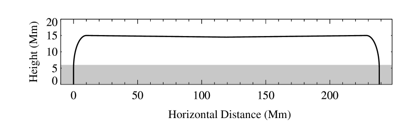
Figure 2: Geometry of our model loop, which represents a magnetic field line across a filament thread. The gray rectangular region denotes the photosphere and the chromosphere. Note that the vertical and the horizontal axes are not to scale.

We adopt a loop geometry with a magnetic dip, which is symmetric about the midpoint. On each side, the loop has a vertical leg of 5 Mm in length above the footpoint and a quarter-circular arc of 15.7 Mm in length connecting the vertical leg and the dip, which is 218.6 Mm in length, as shown in Figure 2. Note that the geometry of the loop determines the distribution of $g_{\parallel}(s)$, which is symmetric about the midpoint and whose left half is described as follows:

$$g_{\parallel}(s)=\cases{-g_{\odot},&$s\leqslant s_{1}$;\cr-g_{\odot}\cos\left(\frac{\displaystyle\pi}{\displaystyle 2}\frac{\displaystyle s-s_{1}}{\displaystyle s_{2}-s_{1}}\right),&$s_{1}<s\leqslant s_{2}$;\cr g_{\odot}\frac{\displaystyle\pi D}{\displaystyle 2(L/2-s_{2})}\sin\left(\pi\frac{\displaystyle s-s_{2}}{\displaystyle L/2-s_{2}}\right),&$s_{2}<s\leqslant L/2$,\cr}$$ (4)

where $g_{\odot}=2.7\times 10^{4}$ cm s^-2 is the solar gravity, $s_{1}=5$ Mm, $s_{2}=s_{1}+15.7$ Mm, $L=260$ Mm is the total loop length, and $D=0.5$ Mm is the dip depth. The value of total loop length $L$ is suggested by the observations of Okamoto et al. (2007). The dip is very shallow, so the coronal part of the loop is nearly flat. The midpoint of the loop, which is the center of the dip, has a height of 14.5 Mm above the bottom boundary.

The initial equilibrium state is obtained by numerically solving Equations (1–3). We start with a temperature ($T$) versus height ($h$) distribution of $T=\tanh(h-h_{0})$ with $T=10^{6}$ K in the corona and 6000 K in the photosphere, which is close to the quiet Sun atmospheric model (Vernazza et al., 1981). The density is determined by balancing the pressure gradient with the gravity, with $n_{H}=\rho/(1.4m_{p})=10^{9}$ cm^-3 at the loop center. At this stage, only the background heating $H_{0}(s)$ is included in the energy equation, namely $H(s)=H_{0}(s)$ in Equation (3). $H_{0}(s)$ is a steady term in order to maintain the hot corona, whose physics is still under debate. Considering that the photospheric motions are the source of the energy that is transported upward to heat the chromosphere and the corona somehow, it is generally conjectured that the heating rate decays with height (Serio et al., 1981; Mok et al., 1990; Aschwanden & Schrijver, 2002). Similar to previous works, we assume that $H_{0}(s)$ exponentially decreases with the distance away from the nearest footpoint along the loop, and remains constant in time:

$$H_{0}(s)=\cases{E_{0}\exp(-s/H_{m}),&$s<L/2$;\cr E_{0}\exp[-(L-s)/H_{m}],&$L/2\leqslant s<L$,\cr}$$ (5)

where the amplitude $E_{0}=3\times 10^{-4}$ ergs cm^-3 s^-1 (Withbroe & Noyes, 1977), and the scale length $H_{m}=L/2$ (Withbroe, 1988). The prescribed distributions are in force equilibrium, but not in thermal equilibrium, and will evolve to reach a new hydrostatic state. Such a state, whose density and temperature distributions are displayed in Figure 3, serves as the initial conditions for our further simulations. In the initial state, the temperature is the highest at the midpoint of the loop, with $T=2.6\times 10^{6}$ K and $n_{H}=3.2\times 10^{8}$ cm^-3. The thin transition layer between the low atmosphere and the corona is roughly at a height of $s_{tr}=6$ Mm. In the low atmosphere, $T$ ranges from 13000 K to 18000 K, which is closer to the quiet Sun atmospheric model (Vernazza et al., 1981) than previous works (Karpen et al., 2001, 2006). The number density at the endpoints is about $2\times 10^{14}$ cm ^-3. The simulated chromosphere and photosphere are about twice thicker than the real Sun, and serve as a mass reservoir for the chromospheric evaporation.

For the boundary conditions, we fix the density, velocity, and temperature at the two endpoints of the loop. Because the density in the photosphere is more than 4 orders of magnitude higher than those in the filaments and the corona, the coronal dynamics has little effect on the photosphere, justifying these fixed boundary conditions.

Similar to Antiochos et al. (1999), in order to simulate the chromospheric evaporation, an extra localized heating $H_{l}(s)$, which might be due to chromospheric reconnection, is added to the energy equation in addition to the background heating $H_{0}(s)$, namely $H(s)=H_{0}(s)+H_{l}(s)$ in Equation (3). As described as follows, $H_{l}(s)$ is uniform in the photosphere and chromosphere, and decays exponentially with the distance away from the nearest chromosphere along the loop with a scale length $\lambda$:

$$H_{l}(s)=\cases{E_{1},&$s\leqslant s_{tr}$;\cr E_{1}\exp[-(s-s_{tr})/\lambda],&$s_{tr}<s\leqslant L/2$;\cr fE_{1}\exp[-(L-s_{tr}-s)/\lambda],&$L/2<s\leqslant L-s_{tr}$;\cr fE_{1},&$s>L-s_{tr}$,\cr}$$ (6)

where the amplitude $E_{1}=10^{-2}$ergs cm^-3 s^-1 (cf. Withbroe & Noyes, 1977; Aschwanden, 2001), $s_{tr}=6$ Mm is the height of transition region, and the factor $f$ is the ratio of the localized heating rate near the right footpoint to that near the left. The localized heating $H_{l}(s)$ is ramped up linearly over 1000 s, and maintained since then. In this paper, we numerically investigate two situations, with symmetric and asymmetric heating, respectively. The parameters in several typical cases are listed in Table 1. In the symmetric case, a parameter survey is performed, including the effects of $\lambda$ and $E_{1}$.

To better identify in which way our simulations augment the knowledge gained in prominence formation over the last decade, we list the most important parameters in similar works on radiative condensation due to localized heating in Tables 2-3. These tables show that our work differs in a variety of aspects, connected to the overall loop geometry, to the spatio-temporal prescription of the heating applied, and also notably in the cooling table used to quantify radiative losses. Motivated by observations of active region prominences by Okamoto et al. (2007), our model loop shape represents a low-lying, shallowly-dipped loop with a more realistic scale for its vertical legs and chromospheric height region. In this shallow dip configuration, our parametric survey explores a wide range in the heating parameters.

3 Numerical Results

3.1 Symmetric Evolution

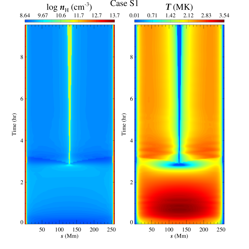
Figure 4: Temporal evolution of the number density of hydrogen (left) and the temperature (right) along the model loop in case S1. The two loop footpoints are at $s=0$ and $260$ Mm, respectively, and the center of the loop dip is at $s=130$ Mm.

As the symmetric localized heating with $\lambda=10$ Mm and $f=1$ is introduced in case S1, the chromospheric plasma is heated and evaporated into the corona. As illustrated by Figure 4, both the density $\rho$ and temperature $T$ in the coronal portion increase accordingly. Near the midpoint of the loop, $T$ reaches the maximum value, $3.49\times 10^{6}$ K, at $t=2664$ s, then starts to decline slowly, whereas $\rho$ keeps increasing slowly from the beginning. At $t=10013$ s, the temperature and the pressure near the midpoint begin to collapse simultaneously, drastically decreasing by nearly one and a half orders of magnitude within 1 min, creating a low pressure cold region, which expands to a maximum length of 28.4 Mm. At this stage, the density is still low, increasing gently as seen from the left and the middle columns of Figure 5. Since only the density is chosen to automatically refine the mesh and at this stage the density is still smooth, the grid resolution is 108 km per cell. Even though, this cold region contains 263 grid cells, which are sufficient to resolve the region. Due to the large pressure gradient that forms at the edge of this cold region, the coronal plasma outside the cold region is driven to move rapidly towards this central cold region. Since time $t=10082$ s, the density inside this cold well begins to increase rapidly as the inflows from two sides converge towards the midpoint and compress the cold region. The converging velocity reaches 185 km s^-1. These inflows are supersonic with a local Mach number up to 7.

As a result, the inflows collide at the midpoint of the loop where a high pressure peak appears, exciting two rebound shock waves launched from the midpoint towards the two sides. A small cold condensation region ($\sim 1$ Mm in length) is left behind the shocks near the midpoint at $t\sim 10382$ s (see the right column of Figure 5). To see the contributions of the various terms in the energy equation, in Figure 6 we plot the absolute value distribution of the energy source terms, including the radiative cooling, the heat conduction, the heating, and the gravity potential, across the magnetic dip at $t=10382$ s, when the condensation happens. It is found that the radiative cooling dominates in the coronal parts and the boundaries of the condensation segment, but nearly vanishes inside the condensation. The heat conduction is less important than the heating in most regions except at the boundaries of the condensation. The gravity potential is always negligible. The pressure in the cold region recovers due to the compression of the inflows from outside. Swept by the outward-propagating rebound shock waves, the depressed pressure outside the cold region also recovers, as illustrated by Figure 7 showing similar quantities at times later than those of Figure 5. The shock waves are bounced back and forth for $\sim 3$ times between the loop footpoint and the loop center, as revealed by the sinusoidal pattern in the right panel of Figure 4 between $t=3$ hr and $t=4$ hr. During their passage, they dissipate their energy to compress and heat the local plasma. The damping rate is enhanced by thermal conduction and radiation. The plasma condensation remains near the midpoint, with a temperature of $1.8\times 10^{4}$ K and a density of $1.2\times 10^{11}$ cm^-3. As a contrast, the corresponding values in the neighboring corona are $2\times 10^{6}$ K and $1.03\times 10^{9}$ cm^-3, respectively. Note that the condensation temperature is just below 20000 K, where the radiative loss is set to vanish smoothly. Further tests indicate that if the radiative losses vanish below a lower temperature, the condensation would be cooler accordingly.

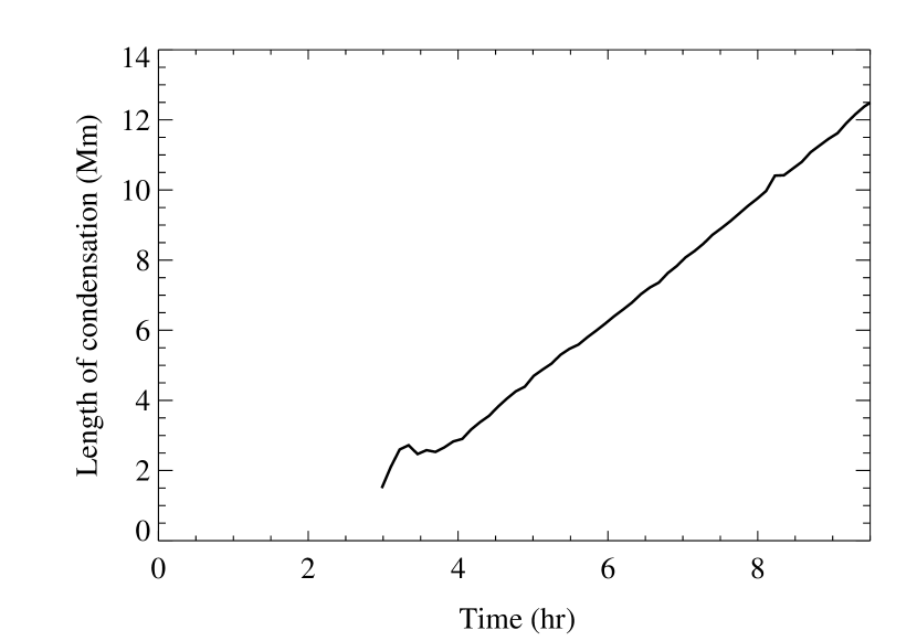
Figure 8: Temporal evolution of the length of the condensation in case S1. The starting point of the line marks the onset of the plasma condensation.

Figure 8 depicts the growth of the condensation segment (or the filament thread). It is seen that the onset time of the condensation is at $t=2.8$ hr after the localized heating is introduced in case S1. The growing process of the condensation can be described as follows: Its length increases rapidly for $\sim 20$ min as the onset of condensation drives fast evaporation flows from the chromosphere, which is followed by a slight shrinkage of the condensation for $\sim 10$ min. As the evaporated plasma flow becomes steady, the condensation length increases linearly with time, with a growth rate of 1511 km hr^-1. With such a speed, it would take $\sim 6.6$ hr to form a filament thread with a typical length of 10 Mm. Observations show that active region filaments form within a day (Wang & Muglach, 2007). For comparison, in Antiochos et al. (1999), it takes 8.3 hr for a condensation to grow to 10 Mm long. One reason is that they used a deeply dipped magnetic loop, where the gravity scale height was shorter, so that the condensation was strongly squeezed.

To investigate the effect of the heating scale length $\lambda$, we change its value and perform a series of simulations in 17 runs, with other parameters the same as in case S1. As seen from Figure 9, the onset time of the condensation roughly increases with $\lambda$, with a minimum of 2 hr. However, the growth rate decreases with increasing $\lambda$, except a drop down near $\lambda=4$ Mm. It is noted that if $\lambda$ is larger than 9 Mm, i.e., 1/28 of the total loop length $L$, the evolution is similar to case S1 (where $\lambda=10$ Mm) as described above, where only a single condensation forms near the midpoint of the loop. When 3 Mm $<\lambda<$ 9 Mm, i.e., $1/86<\lambda/L<1/28$, two condensation segments would form first on the two shoulders of the magnetic dip symmetrically about the midpoint. The two segments move convergently towards the midpoint, during which both $T$ and $p$ in the region between the two segments drop down. Under this pressure gradient, the two condensation segments are accelerated from $\sim 12$ km s^-1 to 75 km s^-1, to finally coalesce near the midpoint. Similar high-speed motion is discussed by Karpen et al. (2006). As $\lambda$ decreases, the two segments form further away from each other and from the midpoint of the loop. When 2.5 Mm $<\lambda<$ 3 Mm, the two condensation segments form in the loop legs and then drain down rapidly to the nearby footpoints. When $\lambda<2.5$ Mm, i.e., $\lambda/L<1/100$, no condensation forms, and the loop relaxes to a hydrostatic state in the end. Similar situations happen when $\lambda>25$ Mm, i.e., $\lambda/L>1/10$, which is the same result mentioned by Klimchuk et al. (2010).

Müller et al. (2004) simulated the formation of condensations in a semicircular coronal loop with a length of 100 Mm and the loop top temperature of $6.8\times 10^{5}$ K. Their loops are shorter and cooler than our dipped loops. They found that when $\lambda/L=1/20$, only one condensation forms at the midpoint of the loop and that two condensation segments form at shoulders of the loop when $\lambda/L=1/33$ or $\lambda/L=1/50$. The transition between one condensation and two condensation segments is somewhere between $\lambda/L=1/20$ and $1/33$, which is consistent with our result, i.e., $1/28$. The transition can be understood as follows: At the beginning, the plasma at the two shoulders of the loop is cooler and denser than that at the midpoint, which means the radiative loss is stronger at two shoulders. Meanwhile, if $\lambda$ is long enough, the heating at shoulders is strong enough to slow down the cooling making the midpoint to be the fastest cooling place, and only one condensation forms. When $\lambda$ decreases, the heating at shoulders is reduced and become too weak to obstruct the fast cooling there. Hence,two cold segments are formed at the two shoulders before merging near the midpoint of the loop.

Keeping $\lambda=10$ Mm, we perform another series of simulations with different amplitude of the localized heating, $E_{1}$, i.e., 0.005–0.2 ergs cm^-3 s^-1. So the localized heating still dominates compared to the weak background heating. The evolution is similar to case S1, such that only one condensation forms near the midpoint. As indicated by Figure 10, the onset time of the condensation decreases as $E_{1}$ increases, whereas the growth rate of the condensation is maximal at $E_{1}\sim 0.01$ ergs cm^-3 s^-1. It is easy to understand that the condensation forms earlier with a larger $E_{1}$ since a stronger chromospheric heating leads to stronger evaporation. The growth rate might be determined by the compromise between the evaporation rate and the deposited energy. A stronger heating drives stronger chromospheric evaporation on one hand, and refrains the evaporated plasma from cooling on the other hand. Another important factor is that the plasma density in the condensation segment increases due to higher compression as $E_{1}$ increases. It becomes slower for a denser condensation to grow. As a combined result, the growth of the condensation peaks at $E_{1}\sim 0.01$ ergs cm^-3 s^-1, and decreases at larger $E_{1}$.

Comparing the onset time and growth rates deduced from observations may help to further pin down the properties of the employed localized heating. However, to determine the onset time of the thread formation requires combined spectral and imaging observations with high resolution, which are not available yet. The growth speed of the filament thread can be compared with future observations.

3.2 Asymmetric Evolution

It is more general that the localized heating in the chromosphere is not symmetric between the two footpoints of a magnetic loop. In this subsection, we perform three simulations with different $f$, the ratio of the heating rate at the right footpoint to the left.

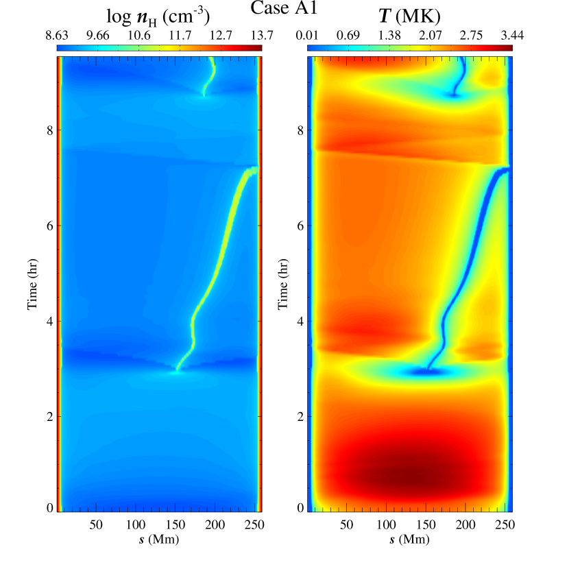
Figure 11: Temporal evolution of the number density of hydrogen (left) and the temperature (right) along the model loop in case A1. The loop footpoints are at $s=0$ and $260$ Mm, respectively, and the center of the loop dip is at $s=130$ Mm.

In case A1, we set $f=0.75$, and other parameters are the same as in case S1. The details of the formation process are similar to case S1, as illustrated by Figure 11, which depicts the time evolution of the density (left panel) and temperature (right panel) distributions. At $t=10690$ s, i.e., 2.97 hr, a condensation with low temperature and high density is formed in the right part, i.e., the less heated part, of the magnetic dip, which is 22.5 Mm away from the midpoint. The distributions of various quantities, e.g., the temperature ($T$), the density ($n$), the pressure ($p$), and the in situ Mach number ($M$), across the condensation segment at three times are shown in Figure 12. It is seen that as the convergent inflows coalesce in the condensation segment, two rebound shock waves are launched, propagating towards left and right footpoint, respectively. The shock waves are reflected between each footpoint and the condensation for several times before fading away, as also indicated by the sinusoidal pattern in the right panel of Figure 11 near $t=3.5$ hr. A significant difference from case S1, however, is that upon formation, the condensation has a velocity of $\sim 5$ km s^-1, moving to the right, or the less heated side, as illustrated by Figure 11. The rightward-moving condensation is accelerated to 15 km s^-1 due to the pressure gradient on its two sides, but soon it is dragged to decelerate by an inversion of the pressure gradient and even falls back by 2 Mm. The pressure gradient inversion is caused by a pressure increase on the right side of the condensation due to the interaction of a shock wave after it is reflected at the right footpoint, when the left-sided shock has not reached the left footpoint yet. After the left-sided shock wave is reflected from the left footpoint and catches the condensation, the pressure on the left side of the condensation increases and exceeds the pressure on the right side. The condensation is then pushed again by the pressure gradient to move to the right with a velocity of $\sim 8$ km s^-1 until it drains down to the right footpoint of the loop. During the travel, the length of the condensation grows from 0.9 Mm to 7.9 Mm. When the condensation impacts the chromosphere, the collision generates a rebound shock wave, which is bounced back and forth between the two footpoints of the loop as indicated by the sinusoidal pattern in the right panel of Figure 11 near $t=8$ hr. The total lifetime of the condensation is $\sim 4.3$ hr. As the simulation goes on, the formation and the drainage of condensation repeats, with a period of 5.5 hr, which is significantly shorter than the 22.8 hr simulated by Karpen et al. (2006). Since the radiative loss coefficent we used is generally $\sim 2$ times larger than theirs, the cooling is stronger and the condensations form faster, which shortens the period of the formation-drainage cycle.

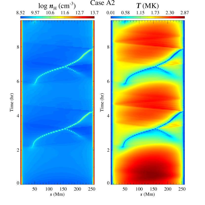
Figure 13: Temporal evolution of the number density of hydrogen (left) and the temperature (right) along the model loop in case A2. The two loop footpoints are at $s=0$ and $260$ Mm, respectively, and the center of the loop dip is at $s=130$ Mm.

As mentioned in subsection 3.1, two condensations can be formed when the heating scale length $\lambda$ is small. Therefore, in case A2, we take $f=0.4$ and $\lambda=5$ Mm. As illustrated by Figure 13, a condensation forms at $t=2.2$ hr near the left shoulder of the magnetic dip ($s=42.1$ Mm) with an initial speed of 10 km s^-1. It is accelerated during its travel towards the right part of the loop, with its length growing up to 5.8 Mm. At $t=2.84$ hr (38 min later), a second condensation, which is smaller than the first one, is formed near the right shoulder of the magnetic dip ($s=205.5$ Mm) with an initial speed of 24 km s^-1 towards the left. The left and the right condensation segments are accelerated for 24 min to 60 km s^-1 and 50 km s^-1, respectively, and then collide at $s=158$ Mm (at the right part of the loop). Two shock waves are generated by the collision, which are then reflected back and forth between the condensation and each footpoint, as revealed by the sinusoidal pattern in the right panel of Figure 13 near $t=3.5$ hr. After the collision, the two condensation segments merge into one, with a length of 2.3 Mm. The coalesced condensation moves to the right with an initial velocity of 32 km s^-1. It is decelerated to 16 km s^-1 at $s=216$ Mm, and then accelerated to 24 km s^-1 with a length of 6 Mm before it drains down to the right footpoint of the loop. The deceleration and acceleration of the condensation is mainly due to the inversion of the pressure gradient caused by the same reason as discussed in case A1, while the gravity effect is small in this shallow dip configuration. The falling down of the condensation excites a shock wave, which is trapped to propagate back and forth in the whole loop as indicated by the right panel of Figure 13 near $t=5$ hr. As time goes on, such a formation, coalescence, and drainage of condensations repeat with a period of 3.6 hr, which is shorter than that in case A1.

As an extreme case, we perform a simulation with $f=0$, i.e., the localized heating is introduced at the left footpoint only. It is found that no condensation forms in the loop. Instead, we get steady flows along the coronal loop, consistent with previous works (e.g., Patsourakos et al., 2004).

4 Discussions

4.1 Thermal Instability

Parker (1953) proposed that some solar activities, such as filaments, can be formed by thermal instability. He derived a criterion for thermal instability on the basis of an analysis of the energy equation alone. Field (1965) made a detailed research of the thermal instability for an infinite, uniform, static plasma in initial thermal equilibrium. He pointed out that the criterion given by Parker is based on the isochoric assumption, i.e., the density is constant in the whole region, which is not compatible with the force equation since the cooling would lead to pressure deficit, which would destroy the initial force balance. He derived an isobaric criterion for the thermal instability, which is consistent with the force equation. The thermal instability was further studied by many other colleagues (e.g., van der Linden & Goossens, 1991; Meerson, 1996, and references therein). It was pointed out that these modes are the marginal entropy modes which are advected with the local flow velocity (Goedbloed et al., 2010), driven unstable by non-adiabatic processes. The different criteria may be applicable for different astrophysical environments.

According to our simulations, as mentioned in §3.1, during the catastrophic cooling stage, the temperature and the pressure drop rapidly, while the density increases only a little at this stage. Significant density enhancement occurs $\sim 3$ min after the catastrophic cooling. Therefore, in the simulated coronal loop, the thermal catastrophe is more isochoric than isobaric. So we use the isochoric thermal instability criterion derived by Parker (1953) as follows:

$$C\equiv k^{2}-\frac{1}{\kappa}\left(\frac{\partial H(s)}{\partial T}-\frac{\partial R}{\partial T}\right)<0$$ (7)

where $k$ is the wave number of the perturbations, $\kappa$ is the heat conduction coefficient, and $R=n_{\rm H}n_{\rm e}\Lambda(T)$ is the radiative loss. The heat conduction introduces a stabilizing effect. We numerically calculate $\partial R/\partial T$, using the central difference scheme. $\partial H(s)/\partial T$ is zero since the heating depends only on space in our simulations. Perturbations with any resolvable wavelength exist in the simulations. According to Figure 5, the cool region has a width of $\sim 10$ Mm, therefore, we take the wavelength of the temperature perturbation as 20 Mm in order to quantify $k$. For small $k$, the occurrence of the thermal instability is mainly determined by the sign of $\partial R/\partial T$.

Taking case S1 as an example, we plot the temporal evolution of the temperature, the density, the pressure, and the isochoric criterion $C$ at the loop midpoint in Figure 14. Since the initial temperature is 2.63 MK, which corresponds to a negative $\partial R/\partial T$, $C=-1.4\times 10^{-15}$ cm^-2 is negative, but very close to 0. Besides, the cooling timescale at this stage is $\sim 10^{4}$ s. Therefore, the early evolution is dominated by the localized heating and chromospheric evaporation. As more mass is filled into the corona, radiation is enhanced gradually, which becomes overwhelming over the heating after $t=2664$ s. The temperature keeps decreasing slowly then. From $t=9850$ s to $t=9994$ s, $C$ becomes positive for a short interval since $T$ falls in the range where $\partial R/\partial T$ is positive. After $t=10013$ s, $C$ drops down drastically to $-1.2\times 10^{-9}$ cm^-2. Simultaneously, the temperature $T$, along with the gas pressure, begins to decrease catastrophically, as indicated by the time derivative of $T$, i.e., the dashed line in the top panel of Figure 14. That is to say, the thermal instability occurs. The temperature drops from $3.4\times 10^{5}$ K to 20000 K in 60 s. However, the density increases by only 20% during this time. Note that $C$ becomes positive out of the plotting range after the catastrophic cooling, corresponding to a thermally stable state. Three minutes later, i.e., at $t=10282$ s, the density increases drastically, and a condensation is then formed. We conclude that the isochoric thermal instability may explain the catastrophic cooling. Such a delay is probably due to the difference between the kinematic timescale and the radiative timescale. It takes an extra 3 min for the plasma to accumulate in the cooling region under the pressure gradient driving.

It might be interesting to check the criterion of the isobaric thermal instability. According to Equation (25) of Field (1965, see also ), the criterion for the thermal instability in the isobaric case is expressed as:

$$C_{\rm isobaric}\equiv\rho\left(\frac{\partial\mathcal{L}}{\partial T}\right)_{\rho}-\frac{\rho^{2}}{T}\left(\frac{\partial\mathcal{L}}{\partial\rho}\right)_{T}+k^{2}\kappa<0$$ (8)

where $\mathcal{L}=(n_{\rm H}n_{\rm e}\Lambda(T)-H(s))/\rho$ is the generalized heat-loss function. For the perturbations with a wavelength of 20 Mm, we calculate the $C_{\rm isobaric}$ at the midpoint of the loop and plot its temporal evolution in the bottom panel of Figure 14. The time when it turns from positive to negative is well before the onset time of the catastrophic cooling. We try many other perturbation wavelengths, and it is found that the isobaric criterion is crucially dependent on the perturbation wavelength while the isochoric criterion is not. Therefore, we conclude that the isobaric thermal instability is not appropriate to explain the catastrophic cooling during the condensation formation in the solar corona.

4.2 Is Continued Heating Necessary?

As mentioned in §1, it has been demonstrated that the extra heating localized in the low atmosphere would drive chromospheric evaporation flows, leading to the plasma condensation in the corona due to thermal instability or loss of thermal equilibrium. In the previous studies, the localized heating is either continuous (Antiochos et al., 1999) or intermittent (Karpen & Antiochos, 2008). In the steady heating case, the condensation can form and grow rapidly, as also demonstrated in this paper. In the successive impulsive heating case, it was found that a condensation can also form steadily when the average interval between heating pulses is less than the coronal radiative cooling time ($\sim 2000$ s, Karpen & Antiochos, 2008). From the theoretical point of view, the localized strong heating may be due to low atmospheric activities, such as chromospheric reconnection. It is quite possible that such a heating event has a finite lifetime and might not show up again at the footpoint of one flux tube. Therefore, it is interesting to see the response of the coronal loop to a single heating event. To do that, we make a numerical experiment, and stop the localized heating 8 minutes after the condensation is formed at $t$=2.87 hr in the symmetric case S1, which means there is only background heating $H_{0}(s)$ in the heating term $H(s)$ in Equation 3, which changes slightly with the distance along the loop. Note that, in order to make the evolution more smooth, the heating is turned off linearly over 1000 s. We find that after the heating ceases, there is still mass upflows from the footpoint to the coronal portion of the loop. For comparison, Figure 15 plots the evolutions of the mass flux from the two shoulders of the magnetic dip to the condensation segment in the steady case (top panel) and the finite-time heating case (bottom panel). It is seen that after the condensation is formed at $t=2.87$ hr, the mass flux oscillates heavily and then maintains at a level of $1.5\times 10^{-8}$ g cm^-2 s^-1 in the steady heating case. However, in the finite-time heating case, the mass flux drops abruptly, but then still maintains at a level of $5.6\times 10^{-10}$ g cm^-2 s^-1 even after the localized heating is removed permanently. That is to say, the mass flux decreases by 27 times, but does not vanish. Such a mass flux corresponds to a growth rate of the condensation length of 230 km hr^-1, which decreases by 6.6 times compared to the steady heating case. The reason why the growth rate does not decrease proportionally with the mass flux is that the plasma density of the condensation is reduced after the heating is switched off.

Therefore, it seems that the evaporation-driven condensation can serve as the trigger of the formation of the filament threads, and there exists a condensation instability. Once the condensation is formed in a small segment near the dip of a coronal loop by the evaporation flow, the condensation will grow, and there is continual mass supply siphoned from the chromosphere, although the growth rate is $\sim 6.6$ times smaller than in the steady heating case.

In order to understand the mechanism of the spontaneous siphon flow after the localized heating is halted, we plot in Figure 16 the time evolution of the gas pressure at the midpoint of the loop, where the condensation is located. It is revealed that after the localized heating is turned off gradually, the pressure at the loop midpoint drops down from $t=3.03$ hr. After several hours of small-amplitude oscillations, the pressure remains at 0.2 dyn cm^-2, which is about half of its initial value 0.37 dyn cm^-2 at $t=0$. Therefore, our simulation result indicates that after thermal instability and plasma condensation, the gas pressure of the cold plasma is reduced, compared to the hot plasma at the same site in the initial hydrostatic state, which leads to a pressure gradient along the loop. It is such a pressure gradient that drives the spontaneous siphon flow, which makes the condensation continue to grow even after the localized heating is switched off.

4.3 Stability to p-mode wave perturbations

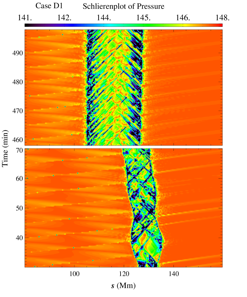
Figure 18: Temporal evolution of Schlierplot of the pressure in the region around the condensation. The lower part shows the initial drifting phase and the upper part shows the final stable phase.

While the previous section demonstrated that prominence growth will continue even after finite-time localized heating, another aspect worth studying is the fate of the prominence condensations subjected to wave buffeting. Since 5-minute solar p-mode oscillations are ubiquitous in the photosphere, it is relevant to investigate whether prominences will be influenced by wave driving, and how they channel (linear) wave modes. Since there is large interest in prominence seismology (see, e.g., the review by Mackay et al., 2010), we now investigate how filaments, once formed, behave under p-mode wave driving, which is denoted as case D1. Case D1 is based on the simulation results of the symmetric case S1, with an initial state taken from 7.1 hours in the evolution shown in Figure 4. We then introduce a sinusoidal velocity perturbation with the amplitude of 1 km s^-1 and the period of 5 minutes. We add this perturbation only at the left footpoint of the loop. The p-mode waves propagate upward through the transition region into the corona and steepen into shocks. A snapshot of the velocity distribution after 509 minutes is shown in Figure 17, where two shock fronts can be identified to the left of the central condensation. The shocks damp in the corona while propagating with a speed of 213 km s^-1, which is close to the local sound wave speed. These shocks hit the condensation and penetrate into it with little reflection, becoming ordinary linear sound waves while propagating through the filament. When these sound waves hit the other boundary of the condensation, they are mainly reflected, with a weak leakage out to the right part of the loop. This is best visualized using a Schlieren plot of the pressure, as shown in Figure 18. This Schlieren plot of the pressure zooms in around the condensation, and actually quantifies the local value of $\exp(-0.01[\left|\nabla p\right|-500])$. The bottom part of Figure  18 shows the first series of shocks hitting the condensation. One notes that the overall thermodynamical changes induce a leftward drift of the central prominence. The symmetry is hereby broken due to our asymmetric driving. During the leftward drifting, the filament thread becomes longer due to the chromospheric evaporation as in case S1. The top panel of Figure 18 shows that ultimately the filament settles down at a quasi-permanent location determined by the overall pressure balance, as altered by the periodic driving. The wave mode reflections and transmissions at the left and right edges of the filament thread can be clearly detected. The different slope of the wave fronts within the filament is due to the lower sound speed there. All these waves, either inside or outside the filament thread, have a 5-min period. The impinging waves are clearly nonlinear, while the internal wave modes are primarily linear, and the transmitted waves are further attenuated. During the entire period simulated, the condensation maintains thermally stable under the perturbation and energy damping from p-mode waves.

4.4 Summary of new findings

Our model is appropriate for low-lying, shallowly-dipped loops, which have not been studied before. Such shallow dip configurations facilitate higher speeds for displacing the condensations. As advocated by studies of hydrostatic coronal loops by Aschwanden & Schrijver (2002), our background heating uses an exponential height dependence, differing from the uniform prescription used in previous works. In case S1, the great details of the condensation process are shown for the first time. Our parameter survey finds new complicated cycles of paired filament formation, with high-speed converging condensations in case A2, with strong-asymmetry and short-scale localized heating. With the improved cooling table, we allow for stronger radiative cooling and therefore find shorter formation time scales compared to previous works. Besides continuous localized heating, the case with finite duration, which is more realistic in the solar atmosphere, is investigated for the first time, which indicates that the extra strong heating is unnecessary to maintain growth of condensations after their onset. We studied the dependence of the formation process for a large parameter range of the heating scale length $\lambda$ and the heating amplitude $E_{1}$. It is found that shorter $\lambda$ or stronger $E_{1}$ can make condensations form earlier, say, $\sim$2 hr after the introduction of the localized heating. Shorter $\lambda$ also leads to faster growth of the condensation. Moreover, the effect of $p$-mode waves is studied for the first time in this context.

5 Conclusions

It has been suggested that localized heating in the chromosphere can drive plasma evaporation into the corona, and form plasma condensation through thermal instability or loss of thermal equilibrium. In order to investigate the details of this process, in this paper we performed 1D radiative hydrodynamic simulations in a magnetic loop, where heat conduction, radiative losses, and heating terms are included in the energy equation. The main results can be summarized as follows:

(1) The cold condensation formation can be divided into three stages, namely, a thermal rearrangement stage, a thermally unstable stage, and a kinematic stage. In the first stage, as more chromospheric mass is evaporated into the corona, the radiative cooling is enhanced, so the temperature decreases slightly and steadily. In the second stage, the criterion of the isochoric thermal instability is satisfied, and both the plasma temperature and pressure drop down rapidly. They reach their minimum in $\simeq 1$ min. In the third stage, strong inflows due to huge pressure gradient are driven towards the cold region. They collide, launching shock waves after forming a condensation in $\sim 3$ min. The 3-min delay of the condensation formation with respect to the catastrophic cooling relates to the longer kinematic timescale of the plasma than the cooling timescale.

(2) When the localized steady heating at the two footpoints is symmetric, one cold plasma condensation forms at the midpoint of the loop, and grows steadily. Our parameter survey indicates that the onset time of the condensation varies from $t=$2 hr to $t=$5 hr, and the mean growth rate varies from 800 km hr^-1 to 4000 km hr^-1, depending on the amplitude and the scale length of the heating function.

(3) When the localized heating at the two footpoints is weakly asymmetric, also one condensation forms. However, it is shifted from the midpoint of the loop towards the less heated footpoint. It moves with a velocity of $\sim 15$ km s^-1, and then drains down to the less heated footpoint. When the heating at the two footpoints is strongly asymmetric and the heating scale length is short, two condensation segments form at the two shoulders of the magnetic dip, successively. The two segments move towards each other with a relative velocity of up to 50 km s^-1, which might account for the counter-streaming found in observations. The two segments finally merge into one segment, which moves and then drains down to the less heated footpoint with a velocity up to 24 km s^-1.

(4) As an extreme case, when heating is localized at one footpoint, no plasma condensation can be formed, and only steady flow is obtained along the coronal loop, as also demonstrated by Patsourakos et al. (2004).

(5) It is found that once formed the condensation can grow even if the localized heating ceases, though the growth rate of the condensation length, $\sim 230$ km hr^-1, is $\sim 6.6$ times smaller than in the steady heating case. Our research suggests that there exists a condensation instability, i.e., after thermal instability and plasma condensation, the gas pressure becomes reduced, and the pressure gradient drives spontaneous siphon flows from the chromosphere to the corona, which helps the further growth of the condensation.

(6) The plasma condensation maintain its stability and keeps growing, even when p-mode waves propagate through it. The fact that waves can be transmitted through the filaments is relevant for prominence seismology, although our results are restricted to longitudinal acoustic waves.

It should be noted that our assumptions, such as the fully ionized plasma and the optically thin radiative cooling, may not be appropriate to investigate details of the dense partially ionized plasmas in filaments. The ionization and radiation transfer in the optically thick plasma should be considered in the future to reproduce the observational characteristics of filaments. The effects of the p-mode waves from the photosphere on the formation of filaments will also be investigated. Multi-dimensional MHD simulations are also planned in order to understand the coupling between the plasma and the magnetic field.

Figure 1: The radiative loss coefficient $\Lambda(T)$ vs. $T$ calculated by Colgan et al. (2008) (squares) and our interpolation (solid line). Note that the Klimchuk-Raymond profile (dashed line) shows the piece-wise continuous radiative loss function used in previous works.

Figure 3: Distributions of the temperature (solid line) and the number density of hydrogen (dashed line) along the model loop in the initial hydrostatic state.

Figure 5: Distributions of the temperature (solid line, top panel), the density (dashed line, top panel), the pressure (solid line, bottom panel), and the velocity (dashed line, bottom panel) across the loop center in case S1 at three moments, i.e., $t=10013$ s (left column), $t=10082$ s (middle column) and $t=10382$ s (right column).

Figure 6: The absolute value distributions of various energy sources, including the radiative cooling (solid line), the heat conduction (dotted line), the heating (dashed line), and the gravity (dashed dotted line), near the midpoint of the loop at $t=10382$ s in case S1.

Figure 7: Distributions of the temperature (solid line, top), the density (dashed line, top), the pressure (solid line, bottom), and the Mach number (dashed line, bottom) along the loop near the midpoint, at three instants after those shown in Figure 5, namely $t=10451$ s (left column), $t=10588$ s (middle column) and $t=10880$ s (right column), in case S1.

Figure 9: Dependence of the onset time (connected asterisks) and the mean growth rate (connected triangles) of the plasma condensation on the scale height of the localized heating, $\lambda$. Note that the figure is divided into two regions where two condensation segments or one condensation segment forms by vertical lines.

Figure 10: Dependence of the onset time of the condensation (connected asterisks) and the mean growth rate (connected triangles) on the amplitude of the localized heating, $E_{1}$.

Figure 12: Distributions of the temperature (solid line, top), the density (dashed line, top), the pressure (solid line, bottom), and the Mach number (dashed line, bottom) along the loop near the midpoint, at three instants, namely $t=10391$ s (left column), $t=10820$ s (middle column) and $t=11078$ s (right column), in case A1.

Figure 14: Temporal evolution of the temperature, the density, the pressure, the isochoric criterion $C$, and the isobaric criterion $C_{\rm isobaric}$ at the midpoint (solid lines), as well as the time derivative of the temperature (dashed line, top panel). Note that the vertical dotted dashed line denotes $t=10013$ s when the thermal instability begins, and the vertical dotted line denotes the end of catastrophic cooling, $t=10070$ s.

Figure 15: Evolutions of the mass flux from two shoulders of the magnetic dip to the midpoint of the loop in the steady heating case (top panel) and the finite-time heating case (bottom panel). Note that the dashed line at $t=3.03$ hr in the bottom panel marks the moment when the localized heating is switched off, and the inset shows the zoom-in view of the curve from $t=6$ hr to 9 hr. The horizontal thin line indicates the zero level.

Figure 16: Evolution of the gas pressure at the midpoint of the loop in the finite-time heating case. The dashed line indicates $t=3.03$ hr when the localized heating is switched off.

Figure 17: Velocity distribution along the loop at $t=509$ min in case D1.

Table 1: The parameters and results of the typical cases

case	$\lambda$	$f$	$E_{1}$	Mean Growth Rate	Onset Time	Segment
	(Mm)		(erg cm-3 s-1)	(km hr-1)	(s)	Number
S1	10	1	0.01	1928	10340	1
S2	5	1	0.01	3228	7729	1
S3	10	1	0.02	1505	9618	1
A1	10	0.75	0.01	1842	10648	1
A2	5	0.4	0.01	3079	7900	2

Table 2: A list of parameters in simulations of radiative condensation . These relate to the overall assumed loop geometry, quantifying the loop length, the presence of a dip, the length of the loop legs, and the height of the chromosphere.

Reference	$L$	$D$	Vertical Leg	$s_{tr}$	Cross Section
	Mm	Mm	Mm	Mm	(Non)Uniform
Antiochos et al. (1999)	220	5	10	10	U
Antiochos et al. (2000)	320	5	60	50	U
Karpen et al. (2001)	340	no	60	60	U
Karpen et al. (2003)	420	15,10	75	60	U
Müller et al. (2003)	10	no	1	1.6	U
Müller et al. (2004)	100	no	1	1.6	U
Karpen et al. (2005)	405	20	60	60	N
Karpen et al. (2006)	405	20	75	60	U
Karpen et al. (2008)	405	20	75	60	U
Klimchuk et al. (2010)	205	no	50	50	U
Our Cases	260	0.5	5	6	U

Table 3: A list of parameters in simulations of radiative condensation. These relate to the heating adopted, and to the radiative cooling prescriptions.

Reference	$E_{0}$	$E_{1}$	$f$	$\lambda$	Type	Radiation
	erg cm-3 s-1	erg cm-3 s-1		Mm	S/I/F1
Antiochos et al. (1999)	1.5e-5	1.e-3	1	10	S	Old2
Antiochos et al. (2000)	1.5e-5	1.e-3	0.75	10	S	Old
Karpen et al. (2001)	1.5e-4	1.e-3	0.75	10	S	Old
Karpen et al. (2003)	1.5e-4	1.e-2	0.75	10	S	Old
Müller et al. (2003)	no	1.2e-3	1	1.25	S	IE3
Müller et al. (2004)	no	1.2e-3	1	5,3,2	S	IE
Karpen et al. (2005)	1.5e-4	1.e-2	0.75	10	S	KR4
Karpen et al. (2006)	1.5e-4	2.e-2,1.e-2	0.75	5,10	S	KR
Karpen et al. (2008)	1.5e-4	1.e-2	0.75	5,1	I	KR
Klimchuk et al. (2010)	6.e-4	8.e-2	0.5,0.75,0.9	5	S	KR
Symmetric Cases	3.e-4	5.e-3$\sim$0.2	1	3$\sim$20	S/F	Colgan
Asymmetric Cases	3.e-4	1.e-2	0.4,0.75	5,10	S	Colgan

• Steady/Impulsive/Finite heating

• A simple piecewise radiative loss function which is an order of magnitude smaller than the updated Klimchuk-Raymond (KR) version

• Radiative loss included by solving Ionization Equations

• Klimchuk-Raymond radiative loss function

References

- Antiochos et al. (2000) Antiochos, S. K., MacNeice, P. J., & Spicer, D. S. 2000, ApJ, 536, 494
- Antiochos et al. (1999) Antiochos, S. K., MacNeice, P. J., Spicer, D. S., & Klimchuk, J. A. 1999, ApJ, 512, 985
- Aschwanden (2001) Aschwanden, M. J. 2001, ApJ, 560, 1035
- Aschwanden & Schrijver (2002) Aschwanden, M. J. & Schrijver, C. J. 2002, ApJS, 142, 269
- Aulanier et al. (1998) Aulanier, G., Demoulin, P., van Driel-Gesztelyi, L., Mein, P., & Deforest, C. 1998, A&A, 335, 309
- Berger et al. (2008) Berger, T. E., Shine, R. A., Slater, G. L., Tarbell, T. D., Title, A. M., Okamoto, T. J., Ichimoto, K., Katsukawa, Y., Suematsu, Y., Tsuneta, S., Lites, B. W., & Shimizu, T. 2008, ApJ, 676, L89
- Chae et al. (2001) Chae, J., Wang, H., Qiu, J., Goode, P. R., Strous, L., & Yun, H. S. 2001, ApJ, 560, 476
- Choe & Lee (1992) Choe, G. S. & Lee, L. C. 1992, Sol. Phys., 138, 291
- Colgan et al. (2008) Colgan, J., Abdallah, Jr., J., Sherrill, M. E., Foster, M., Fontes, C. J., & Feldman, U. 2008, ApJ, 689, 585
- Dahlburg et al. (1998) Dahlburg, R. B., Antiochos, S. K., & Klimchuk, J. A. 1998, ApJ, 495, 485
- Engvold (2004) Engvold, O. 2004, in IAU Symposium, Vol. 223, Multi-Wavelength Investigations of Solar Activity, ed. A. V. Stepanov, E. E. Benevolenskaya, & A. G. Kosovichev, 187–194
- Field (1965) Field, G. B. 1965, ApJ, 142, 531
- Goedbloed et al. (2010) Goedbloed, J. P., Keppens, R., & Poedts, S. 2010, Advanced Magnetohydrodynamics, (Cambridge University Press)
- Guo et al. (2010) Guo, Y., Schmieder, B., Démoulin, P., Wiegelmann, T., Aulanier, G., Török, T., & Bommier, V. 2010, ApJ, 714, 343
- Jing et al. (2010) Jing, J., Yuan, Y., Wiegelmann, T., Xu, Y., Liu, R., & Wang, H. 2010, ApJ, 719, L56
- Karpen & Antiochos (2008) Karpen, J. T. & Antiochos, S. K. 2008, ApJ, 676, 658
- Karpen et al. (2001) Karpen, J. T., Antiochos, S. K., Hohensee, M., Klimchuk, J. A., & MacNeice, P. J. 2001, ApJ, 553, L85
- Karpen et al. (2006) Karpen, J. T., Antiochos, S. K., & Klimchuk, J. A. 2006, ApJ, 637, 531
- Karpen et al. (2003) Karpen, J. T., Antiochos, S. K., Klimchuk, J. A., & MacNeice, P. J. 2003, ApJ, 593, 1187
- Karpen et al. (2005) Karpen, J. T., Tanner, S. E. M., Antiochos, S. K., & DeVore, C. R. 2005, ApJ, 635, 1319
- Keppens et al. (2003) Keppens, R., Nool, M., Tóth, G., & Goedbloed, J. P. 2003, Computer Physics Communications, 153, 317
- Keppens et al. (2011) Keppens, R., Meliani, Z., van Marle, A.J., Delmont, P., Vlasis, A., & van der Holst, B. 2011, J. Chem. Phys., in press (doi:10.1016/j.jcp.2011.01.020)
- Kippenhahn & Schlüter (1957) Kippenhahn, R. & Schlüter, A. 1957, Zeitschrift fur Astrophysik, 43, 36
- Klimchuk et al. (2010) Klimchuk, J. A., Karpen, J. T., & Antiochos, S. K. 2010, ApJ, 714, 1239
- Kuperus & Raadu (1974) Kuperus, M. & Raadu, M. A. 1974, A&A, 31, 189
- Lin et al. (2005) Lin, Y., Engvold, O., Rouppe van der Voort, L., Wiik, J. E., & Berger, T. E. 2005, Sol. Phys., 226, 239
- Lin et al. (2003) Lin, Y., Engvold, O. R., & Wiik, J. E. 2003, Sol. Phys., 216, 109
- Litvinenko & Wheatland (2005) Litvinenko, Y. E. & Wheatland, M. S. 2005, ApJ, 630, 587
- Löhner (1987) Löhner, R. 1987, Comp. Meth. in Appl. Mech. and Engineering, 61, 323
- López Ariste et al. (2006) López Ariste, A., Aulanier, G., Schmieder, B., & Sainz Dalda, A. 2006, A&A, 456, 725
- Mackay (2005) Mackay, D. H. 2005, in Astronomical Society of the Pacific Conference Series, Vol. 346, Large-scale Structures and their Role in Solar Activity, ed. K. Sankarasubramanian, M. Penn, & A. Pevtsov, 177–+
- Mackay et al. (2010) Mackay, D. H., Karpen, J. T., Ballester, J. L., Schmieder, B., & Aulanier, G. 2010, Space Sci. Rev., 151, 333
- Malherbe (1989) Malherbe, J. 1989, in Astrophysics and Space Science Library, Vol. 150, Dynamics and Structure of Quiescent Solar Prominences, ed. E. R. Priest, 115–141
- Meerson (1996) Meerson, B. 1996, Reviews of Modern Physics, 68, 215
- Mok et al. (1990) Mok, Y., Drake, J. F., Schnack, D. D., & van Hoven, G. 1990, ApJ, 359, 228
- Müller et al. (2003) Müller, D. A. N., Hansteen, V. H., & Peter, H. 2003, A&A, 411, 605
- Müller et al. (2004) Müller, D. A. N., Peter, H., & Hansteen, V. H. 2004, A&A, 424, 289
- Okamoto et al. (2007) Okamoto, T. J., Tsuneta, S., Berger, T. E., Ichimoto, K., Katsukawa, Y., Lites, B. W., Nagata, S., Shibata, K., Shimizu, T., Shine, R. A., Suematsu, Y., Tarbell, T. D., & Title, A. M. 2007, Science, 318, 1577
- Parker (1953) Parker, E. N. 1953, ApJ, 117, 431
- Patsourakos et al. (2004) Patsourakos, S., Klimchuk, J. A., & MacNeice, P. J. 2004, ApJ, 603, 322
- Poland & Mariska (1986) Poland, A. I. & Mariska, J. T. 1986, Sol. Phys., 104, 303
- Priest (1988) Priest, E. R. 1988, Dynamics and Structure of Quiescent Solar Prominences, (Kluwer Academic Publishers)
- Priest et al. (1996) Priest, E. R., van Ballegooijen, A. A., & Mackay, D. H. 1996, ApJ, 460, 530
- Schmieder et al. (2010) Schmieder, B., Chandra, R., Berlicki, A., & Mein, P. 2010, A&A, 514, A68+
- Schmieder et al. (1991) Schmieder, B., Raadu, M. A., & Wiik, J. E. 1991, A&A, 252, 353
- Serio et al. (1981) Serio, S., Peres, G., Vaiana, G. S., Golub, L., & Rosner, R. 1981, ApJ, 243, 288
- Tandberg-Hanssen (1995) Tandberg-Hanssen, E. 1995, The Nature of Solar Prominences, (Kluwer Academic Publishers)
- Tóth & Odstrčil (1996) Tóth, G. & Odstrčil, D. 1996, J. Chem. Phys., 128, 82
- Townsend (2009) Townsend, R. H. D. 2009, ApJS, 181, 391
- van Ballegooijen & Martens (1990) van Ballegooijen, A. A. & Martens, P. C. H. 1990, ApJ, 361, 283
- van der Linden & Goossens (1991) van der Linden, R. A. M. & Goossens, M. 1991, Sol. Phys., 131, 79
- van Marle & Keppens (2011) van Marle, A. J. & Keppens, R. 2011, Computer & Fluids, 42, 44
- Vernazza et al. (1981) Vernazza, J. E., Avrett, E. H., & Loeser, R. 1981, ApJS, 45, 635
- Wang & Muglach (2007) Wang, Y. & Muglach, K. 2007, ApJ, 666, 1284
- Withbroe (1988) Withbroe, G. L. 1988, ApJ, 325, 442
- Withbroe & Noyes (1977) Withbroe, G. L. & Noyes, R. W. 1977, ARA&A, 15, 363
- Wu et al. (1990) Wu, S. T., Bao, J. J., An, C. H., & Tandberg-Hanssen, E. 1990, Sol. Phys., 125, 277
- Yan et al. (2001) Yan, Y., Deng, Y., Karlický, M., Fu, Q., Wang, S., & Liu, Y. 2001, ApJ, 551, L115
- Zirker et al. (1998) Zirker, J. B., Engvold, O., & Martin, S. F. 1998, Nature, 396, 440