Symmetry and Separation in Surface and Curve Flows

The Role of Symmetry and Separation
in Surface Evolution and Curve Shortening

Philip BROADBRIDGE ^† and Peter VASSILIOU ^‡

P. Broadbridge and P. Vassiliou

^† School of Engineering and Mathematical Sciences, La Trobe University,
^† Melbourne, Victoria, Australia P.Broadbridge@latrobe.edu.au

^‡ Faculty of Information Sciences and Engineering, University of Canberra,
^† Canberra, A.C.T., Australia Peter.Vassiliou@canberra.edu.au

Received January 23, 2011, in final form May 25, 2011; Published online June 01, 2011

With few exceptions, known explicit solutions of the curve shortening flow (CSE) of a plane curve, can be constructed by classical Lie point symmetry reductions or by functional separation of variables. One of the functionally separated solutions is the exact curve shortening flow of a closed, convex “oval”-shaped curve and another is the smoothing of an initial periodic curve that is close to a square wave. The types of anisotropic evaporation coefficient are found for which the evaporation-condensation evolution does or does not have solutions that are analogous to the basic solutions of the CSE, namely the grim reaper travelling wave, the homothetic shrinking closed curve and the homothetically expanding grain boundary groove. Using equivalence classes of anisotropic diffusion equations, it is shown that physical models of evaporation-condensation must have a diffusivity function that decreases as the inverse square of large slope. Some exact separated solutions are constructed for physically consistent anisotropic diffusion equations.

curve shortening flow; exact solutions; symmetry; separation of variables

35A30; 35K55; 58J70; 74E10

1 Introduction

The standard curve shortening flow is a nonlinear evolution by curvature,

$$\frac{\partial\gamma}{\partial t}(x,t)=\kappa(x,t)\mathbf{n}(x,t),\qquad\gamma(x,0)=\gamma_{0}(x),$$ (1)

where $\kappa(x,t)$ is the Euclidean curvature of $\gamma(x,t)$ and $\mathbf{n}(x,t)$ is the outward unit normal to the curve at each point. For the curve-shortening flow parameterized as $x\mapsto(x,y(x,t))$,

$$\mathbf{n}\cdot\mathbf{e}_{y}y_{t}=\mathbf{n}\cdot\frac{\partial\gamma}{\partial t}(x,t),\qquad y_{t}=\frac{y_{xx}}{1+y_{x}^{2}},$$ (2)

which describes the curve shortening flow in Cartesian coordinates. This equation arises in the practical context of metal surface evolution [25]. More recently, it has been used extensively as an isotropic curve-smoothing mechanism in image processing [24, 26]; see also [10]. Equation (1) is well known and has been the subject of several important studies, for instance [17, 18]. Few explicit and exact curve shortening flows of plane curves are known in the literature. Some similarity solutions with prescribed-slope boundary conditions have been constructed parametrically in terms of integrals of algebraic functions of elementary functions [6, 21]. King [22] writes down a number non-invariant solutions. In addition, there are known to be various self-similar rotating spiral and flower-head solutions [2, 19].

We demonstrate in this paper how for most solutions known to us, Lie symmetries of various types or separable coordinate systems play a vital role and we conjecture that all currently known solutions and many new solutions can be obtained via a series of higher order constraints in the method of functional separation. In Section 2 we briefly review the solutions that can be obtained by symmetry reduction. In Section 3, we show how the method of functional separation of variables recovers additional interesting explicit, non-self-similar solutions. Some of the properties and materials science applications of these solutions are developed in more detail. In Section 4, an anisotropic version of the second-order Mullins equation is derived for materials that include a realistic dependence of evaporation coefficient on surface orientation. Equivalence classes for anisotropic evaporation coefficients are constructed under the Euclidean group. Using the equivalence classes, in Section 5 we investigate under which types of anisotropy, analogs of the standard solutions for isotropic diffusion, do or do not exist. Some examples of exact solutions are produced by direct construction and in Section 6 by functional separation of variables.

2 Symmetry reductions of the curve shortening equation

One of the most widely used techniques for constructing explicit, exact solutions of nonlinear partial differential equations is Lie symmetry reduction. This has been extensively investigated in relation to the partial differential equation (2) or its derivative forms

$$u_{t}=\partial_{x}[D(u)u_{x}],\qquad D(u)=1/\left(1+u^{2}\right),$$ (3)

$$\kappa_{t}=\kappa^{2}\kappa_{\theta\theta}+\kappa^{3},$$ (4)

$$R_{t}=\partial_{\theta}[R^{-2}R_{\theta}]-R^{-1},$$ (5)

where $u=y_{x}$, $\kappa$ is curvature, $R=1/\kappa$ and $\theta$ is the orientation angle along a convex curve [3]. Although the standard nonlinear diffusion equation (3) is rarely used in the context of curve shortening, it has non-trivial Lie potential symmetries that enable one to construct exact similarity solutions [5]. The reaction-diffusion equation in standard form (5), another equation that is rarely used in the context of curve shortening, has been fully classified by Lie point symmetry reductions [16].

In common with all autonomous nonlinear diffusion equations of second order, the curve shortening equation (2) is invariant under translations in $x$, $y$ and $t$, plus the Boltzmann scaling group generated by $x\partial/\partial x+y\partial y+2t\partial/\partial t$:

$$(\bar{x},\bar{y},\bar{t})=\big{(}e^{\epsilon}x,e^{\epsilon}y,e^{2\epsilon}t\big{)}.$$

This allows the possibility of two types of scale-invariant similarity solution: the expanding solution of the form $y/\sqrt{t-t_{0}}=G(x/\sqrt{t-t_{0}})$, $(t>t_{0})$ and the contracting solution of the form $y/\sqrt{t_{0}-t}=G(x/\sqrt{t_{0}-t})$, $(t<t_{0})$. Being Euclidean-invariant, (2) has the rotation group as an additional symmetry. Some interesting exact solutions to this equation, and consequently to (3) can be constructed by consecutive symmetry reductions [5]; see also [12].

The expanding homothetic similarity solution with initial-boundary conditions $y_{x}(0,t)=m$, $y\to 0$, $x\to\infty$ and $y(x,0)=0$, was given in [6]. The solution takes the form of the symmetrized (upper) curve in Fig. 1, which represents an evolving grain boundary groove [25, 6].

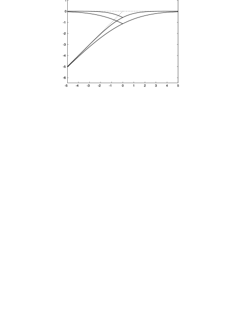
Figure 1: Self-similar evolution by evaporation near a grain boundary groove (symmetrized upper curve) or equivalently by condensation in an obtuse-angled wedge. Output times are at $t=1$ and $t=4$.

Alternatively, the above solution may be extended smoothly to the interior of an obtuse-angled wedge, as shown. These and the homothetic solutions in an acute-angled wedge, obtainable from the same type of reduction, make up the “open-angle” solutions [21].

The homothetically shrinking simple closed-curve solution is the circle $r=\sqrt{2}(t_{0}-t)^{1/2}$. Self-intersecting closed-curve “flower-head” solutions were given in [2].

Steady-state solutions, invariant under time translations, are simply the straight lines. Likewise, the solutions that are invariant under spatial translations in a particular direction are simply the straight lines in that direction. Another simple known solution is the travelling wave solution of the form $y-ct=G(x)$, which is invariant under the translation in space and time generated by $\partial/\partial t+c\partial/\partial y$. This is the well-known “Calabi grim reaper” [18], taking the appearance of a shepherd’s crook

$$y-ct=\frac{-1}{c}\log\cos(cx).$$

Uniformly rotating solutions of the form $r=G(\phi-\sigma t)$ ($r$ and $\phi$ being plane polar coordinates) follow from reduction by the symmetry generated by $\sigma(-y\partial/\partial x+x\partial/\partial y)-\partial/\partial t$.

Expanding or contracting rotating solutions of the invariant form $r/\sqrt{t}=G(\phi-\frac{\sigma}{2a_{3}}\log t)$ or $r/\sqrt{-t}=G(\phi-\frac{\sigma}{2a_{3}}\log(-t))$ follow from reductions under the one-parameter group generated by a linear combination of generators of dilatations and rotations

$$\Gamma=\Gamma_{4}+\sigma\Gamma_{5},\qquad\Gamma_{4}=x\frac{\partial}{\partial x}+y\frac{\partial}{\partial y}+2t\frac{\partial}{\partial t},\qquad\Gamma_{5}=-y\frac{\partial}{\partial x}+x\frac{\partial}{\partial y}.$$

A classification of the types of solutions of the associated reduced ordinary differential equations, but without solving them explicitly and without referring to symmetries, was given recently by Halldorsson [19].

2.1 Reciprocal transformations

It is well known that the class of nonlinear heat equations is stabilised by reciprocal transformations which can sometimes be used to generate new solutions from old [23]. A reciprocal transformation may be viewed as a map of the graph of a solution $u(x,t)$ of

$$u_{t}=(D(u)u_{x})_{x}$$

to that of a solution $u^{\prime}(x^{\prime},t^{\prime})$ of

$$u^{\prime}_{t^{\prime}}=\left(D^{\prime}(u^{\prime})u^{\prime}_{x^{\prime}}\right)_{x^{\prime}}.$$

The map $(x,t,u)\to(x^{\prime},t,u^{\prime})$ is defined by

$$dx^{\prime}=u\,dx+D(u)u_{x}\,dt,\qquad dt^{\prime}=dt,\qquad u^{\prime}=\frac{1}{u}.$$ (6)

It can be shown that this induces the transformation of diffusivities

$$D^{\prime}(s)=\frac{1}{s^{2}}D\left(\frac{1}{s}\right).$$ (7)

The diffusivity of interest here

$$D(u)=\frac{1}{1+u^{2}}$$

is seen to be invariant under the reciprocal transformation,

$$D^{\prime}(u^{\prime})=\frac{1}{1+{u^{\prime}}^{2}}=D(u^{\prime}).$$

This raises the possibility of using the known solutions and generating new solutions of (3) and hence new curve flows by quadrature. However, it turns out that the reciprocal transformation of solutions of (3) acts geometrically trivially on solutions of the curve shortening equation.

Proposition 2.1.

Suppose $u(x,t)$ is a solution of (3) and $y(x,t)$ the corresponding solution of the curve shortening equation. Let $(x^{\prime},t^{\prime},u^{\prime})$ be the reciprocal transformation of $(x,t,u)$. Then the induced transformation on solutions of (2) satisfies $(x^{\prime},t^{\prime},y^{\prime})=(y,t,x+c)$, $c={\rm const}$. That is, for each $t$, the reciprocal transformation of a known solution of (3) induces a reflection $($up to additive constant$)$ of the solution $y(x,t)$ in the line $y=x$.

Proof 2.2.

Equation (3) and the reciprocal transformation (6) permits us to write

$$x^{\prime}=\int_{0}^{x}u(x_{1},t)dx_{1}-\int_{a}^{t}V_{0}(t_{1})dt,$$

where $a$ is a constant and $V_{0}(t)=-D(u(0,t))u_{x}(0,t)$. In terms of Cartesian coordinates $(x,y)$,

$$x^{\prime}=\int_{0}^{x}y_{x}(x_{1},t)dx_{1}-\int_{a}^{t}V_{0}(t_{1})=y(x,t)-y(0,t)+\int_{a}^{t}D(y_{x}(0,t_{1}))y_{xx}(0,t_{1})dt_{1}$$

$$\phantom{x^{\prime}}{}=y(x,t)-y(0,t)+\int_{a}^{t}y_{t}(0,t_{1})dt_{1}=y(x,t)-y(0,a).$$

Then

$$u^{\prime}=1/u=1/y_{x}=x_{y}=x_{x^{\prime}}.$$

Now as $y^{\prime}$ satisfies $y^{\prime}_{x^{\prime}}=u^{\prime}$ just as $y_{x}=u$, then it follows that $y^{\prime}=x+H(t^{\prime})$. However, since $y^{\prime}(x^{\prime},t^{\prime})$ is to satisfy the curve shortening equation

$$y^{\prime}_{t^{\prime}}=\frac{y^{\prime}_{x^{\prime}x^{\prime}}}{1+(y^{\prime}_{x^{\prime}})^{2}},$$

it follows that $H={\rm const}$.

Let $f_{1}$ be a function such that the reflection of its graph defines a function $f_{2}$. In general $f_{1}$ and $f_{2}$ will satisfy different differential equations and this can be very useful. For example, the nonlinear diffusion equation with diffusivity $D(s)=s^{-2}$, seen from (7) to be directly transformable to the classical linear heat equation $(k=1)$, is one of many integrable equations that can be linearized in its potential form by the hodograph transformation [13]: $(x^{\prime},y^{\prime})=(y,x)$ given in Proposition 2.1. However, from a geometric point of view a curve and its reflection are indistiguishable. Thus invariance of (3) under reciprocal transformations does not increase the class of known curve flows. This highlights the difficulty of constructing solutions of the curve shortening equation and partly explains why so few interesting exact solutions are known.

3 Functionally separable nonlinear heat equations

Apart from symmetry methods, one can seek reductions that arise from second or higher order differential constraints rather than the first order differential constraints implied by classical Lie reduction. Unfortunately, there is no general procedure for seeking such reductions and much effort has gone into devising new reduction strategies for partial differential equations. Thus in Doyle and Vassiliou [15] the authors managed to classify all one-dimensional sourceless heat equations

$$u_{t}=(D(u)u_{x})_{x}$$ (8)

that admit separation of variables in some field variable $\bar{u}$. That is, one asks for a change of field variable $\bar{u}=m(u)$, such that the image of (8) under the change of variable, constrained by the additively separable condition

$$\bar{u}_{xt}=0,$$

is a differential system of finite type that can therefore be solved by ordinary differential equations. Indeed the resulting differential system has the general form

$$\bar{u}_{t}=f(\bar{u})\bar{u}_{xx}+g(\bar{u})\bar{u}^{2}_{x},\qquad\bar{u}_{xt}=0,$$ (9)

for some functions $f>0$, $g$. It is proven in [15] that for any such pair $f$, $g$ there is a change of dependent variable that transforms $(\ref{NLheatSep})_{1}$ to (8). It turns out that system (9) has a maximal 3-parameter solution space for any given pair $f$, $g$. In this manner the authors obtain exactly nine distinct diffusivities $D$ up to the maximal transformation group that preserves the canonical form (8) for which the maximal 3-parameter solution space is achieved. In many cases the 3-parameter solution was constructed. This considerably extends the list of nonlinear diffusion equations for which explicit solutions are available. One equation on the Doyle–Vassiliou list is the nonlinear heat equation

$$u_{t}=\left(\frac{u_{x}}{1+u^{2}}\right)_{x}.$$ (10)

Thus the differential 1-form

$$\omega=u\,dx+\frac{u_{x}}{1+u^{2}}\,dt$$

is closed on solutions of (10). It is easy to see that any function $y(x,t)$ satisfying $dy=\omega$ is a solution of the curve shortening equation (2). The solutions of (10) constructed in [15] are the functions

$$u(x,t)=U\big{(}\sigma(x+a),\sigma^{2}(t+b)\big{)},$$

where $a$, $b$ and $\sigma\neq 0$ are arbitrary constants and $U$ is one of the functions

$$U(x,t)=\tan x,$$

$$U(x,t)=\frac{x}{\sqrt{-x^{2}-2t}},$$

$$U(x,t)=\frac{\pm 1}{\sqrt{e^{2(x-t)}-1}},$$

$$U(x,t)=\frac{\sinh x}{\sqrt{-\cosh^{2}x-e^{-2t}}},$$ (11)

$$U(x,t)=\frac{\pm\cosh x}{\sqrt{-\sinh^{2}x+e^{-2t}}},$$

$$U(x,t)=\frac{\sin x}{\sqrt{\cos^{2}x-e^{2t}}},$$

$$U(x,t)=\frac{\sin x}{\sqrt{\cos^{2}x+e^{2t}}}.$$

Each solution (11) provides a 3-parameter family of explicit curve shortening flows except for the complex-valued, $\text{(\ref{DVsols})}_{4}$.

The function $y(x,t$) may be obtained from $U(x,t)$ simply by integrating in $x$, then adding a suitable function of $t$.

1. $\text{(\ref{DVsols})}_{1}$ then leads to the Calabi “grim reaper” travelling wave.

2. $\text{(\ref{DVsols})}_{2}$ integrates to the well-known shrinking circle $x^{2}+y^{2}=2(t_{0}-t)$.

3. Integration of $\text{(\ref{DVsols})}_{3}$ merely produces a horizontal version of the vertical grim reaper.

4. $\text{(\ref{DVsols})}_{4}$ is complex-valued, not considered further in the current practical context.

5. $\text{(\ref{DVsols})}_{5}$ is equivalent to $\text{(\ref{DVsols})}_{7}$ by a rotation in the $xy$-plane.

6. The final two solutions are related to those previously presented by King [22], expressed in the time-reversed form as examples of finger growth; these deserve closer inspection.

3.1 Exact heat flow of a convex curve

The studies of Gage–Hamilton [17] and Grayson [18] on flow by curvature of embedded plane curves is a justly celebrated chapter in differential geometry.

Theorem 3.1 (Gage–Hamilton).

Let $\gamma_{0}:I_{x}\to\mathbb{R}^{2}$ be a convex curve embedded in the plane. Let $\gamma_{0}$ evolve by the curve shortening flow. That is,

$$\frac{\partial\gamma}{\partial t}(x,t)=\kappa(x,t)\mathbf{n}(x,t),\qquad\gamma(x,0)=\gamma_{0}(x),$$

where $\kappa(x,t)$ is the Euclidean curvature of $\gamma(x,t)$. Then the curve remains convex and becomes circular as it shrinks in the sense that

1. the ratio of the inscribed radius to the circumscribed radius approaches $1$;

2. the ratio of the maximum to the minimum curvature approaches $1$;

3. the higher order derivatives of the curvature converge to zero uniformly.

$\text{(\ref{DVsols})}_{6}$ provides the only known example of an explicit, non-self similar curve shortening flow in case the initial curve $\gamma_{0}$ is a closed, convex embedded plane curve which is not a circle. We use results described in Section 2. The sixth function in (11) is

$$u=\frac{\sin x}{\sqrt{\cos^{2}x-e^{2t}}}.$$ (12)

In the case of (12), the corresponding solution of (2) is

$$y=t-\ln\left(\cos x+\sqrt{\cos^{2}x-e^{2t}}\right).$$ (13)

Clearly if $y$ is a solution of (2) then so is $-y$. The two solutions join smoothly along $y=0$ and can be jointly expressed in the simple implicit form

$$\cosh y-e^{-t}\cos x=0.$$ (14)

This solution is recorded in [22] and shown here to arise from functional separation. Solutions of this type are also studied in [14] and referred to as ‘Angenent ovals’, although explicit solutions are not written down in the latter paper. We will now study some properties of this solution. For each $t\in(-\infty,0)$ equation (14) defines a closed, convex “oval-shaped” curve which is symmetric about the $x$- and $y$-axes for

$$x\in\left(-\cos^{-1}\left(e^{t}\right),\cos^{-1}\left(e^{t}\right)\right),\qquad y\in\left(-\cosh^{-1}\left(e^{-t}\right),\cosh^{-1}\left(e^{-t}\right)\right).$$

By analogy with an ellipse, eccentricity may be defined as

$$\epsilon(t)=\sqrt{1-(x_{\max}/y_{\max})^{2}}=\sqrt{1-\left[\frac{\cos^{-1}\left(e^{t}\right)}{\cosh^{-1}\left(e^{-t}\right)}\right]^{2}}=\sqrt{\frac{2}{3}|t|}+O\left(|t|^{3}\right),$$

showing approach to circularity $(\epsilon\to 0)$ as $t$ approaches the extinction time 0. The curvature at each point $(x,t)$ of the curve is

$$\kappa(x,t)=\frac{e^{-t}\cos x}{\sqrt{e^{-2t}-1}}.$$

For each $t\in\left(-\infty,0\right)$, the maximum curvature occurs at $x=0$ with value $\kappa_{\max}=e^{-t}/\sqrt{e^{-2t}-1}$, while the minimum occurs at the extremities along the minor axis, $x=\pm\cos^{-1}\left(e^{t}\right)$ with value $\kappa_{\min}=1/\sqrt{e^{-2t}-1}$. Hence

$$\lim_{t\to 0^{-}}\frac{\kappa_{\max}}{\kappa_{\min}}=\lim_{t\to 0^{-}}e^{-t}=1,$$

verifying the Gage–Hamilton theorem and more specifically showing that the ratio of maximum to minimum curvature is an exponential function converging to unity. Of course, the curvature itself is an unbounded function of time as the flow continues toward extinction.

It transpires that for this curve flow, arclength can be expressed as a function of time in terms of the incomplete elliptic integral of the first kind.

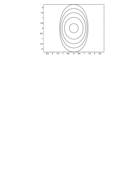
Figure 2: Evolution by heat shrinking flow of the curve defined by $\cosh y-5\cos x=0.$

At very early times $t\ll 0$, the solution with $x\in(-\pi/2,\pi/2)$ is asymptotic to two grim reapers joined smoothly and approaching each other with constant speed:

$$y=\pm(t-\log\cos(x)-\log 2)+O\big{(}e^{4t}\sec^{4}(x)\big{)}.$$

A question that may be posed is: why construct curve shortening flows by first solving (10) rather than solving (2) directly? Remarkably, it can be shown that

Proposition 3.2.

The image of the curve shortening equation (2) under the transformation $y\mapsto m(y)$ does not have a $($maximal$)$ $3$-parameter family of joint solutions with the linear wave equation $y_{xt}=0$ in any field variable $m(y)$ except $m=\text{identity}$ in which case the solution gives rise to the grim-reaper flow.

Proof 3.3.

Construct the image of the curve shortening equation (2) under the change of variable $y\mapsto m(y)$ and apply the Cartan–Kähler theorem to the differential system consisting of the transformed curve shortening equation and the constraint $y_{xt}=0$.

This is in sharp contrast to the rich separability properties of nonlinear heat equations (8) as discussed in Section 2. Thus starting with (10) appears to be an important first step in constructing non-trivial curve flows.

3.2 Decaying periodic solution initially close to square wave

For a curve fixed at two end-points, we prescribe the boundary conditions

$$y=0,\qquad x=0,\ell.$$

We now define dimensionless space and time variables $X=x/\ell$, $Y=y/\ell$, $\tau=Bt/\ell^{2}$, in terms of which the curve shortening equation is

$$Y_{\tau}=\frac{Y_{XX}}{1+Y_{X}^{2}},$$ (15)

to be solved subject to boundary conditions

$$Y=0,\qquad X=0,1$$ (16)

and continuous initial conditions $Y(X,0)=Y_{0}(X).$

Integrating the seventh member of the list (11) and then applying translational and scaling invariance transformations, we obtain

$$Y=\frac{1}{K}\ln\left(\frac{\sqrt{\exp(2K^{2}[\tau-\tau_{0}])+\cos^{2}(K[X-X_{0}])}+\cos(K[X-X_{0}])}{\exp(K^{2}[\tau-\tau_{0}])}\right),$$ (17)

with $K$, $X_{0}$, $\tau_{0}$ arbitrary constants. It may be verified that (17) satisfies (15). In fact, when $\tau-\tau_{0}$ is large and negative,

$$Y=\frac{\ln 2}{K}-K[\tau-\tau_{0}]+\frac{1}{K}\ln\cos(K[X-X_{0}])+O\left(\frac{e^{-2K^{2}[\tau_{0}-\tau]}}{\cos(K[X-X_{0}])}\right).$$

This shows that away from the singularities of $\ln\cos(X-X_{0})$, the solution is asymptotic in the distant past to the Calabi “grim reaper” solution of the curve-shortening flow [18]. At all times, the solution (17) is a deformation of the grim reaper solution but now it is extended smoothly and periodically, without singularities over a domain of any length. Unlike in the grim reaper solution, there are fixed points so that we may apply the Dirichlet boundary conditions (16), which lead to

$$Y=\pm\frac{1}{K}\ln\left(\frac{\sqrt{\exp(2K^{2}[\tau-\tau_{0}])+\sin^{2}(KX)}+\sin(KX)}{\exp(K^{2}[\tau-\tau_{0}])}\right),$$ (18)

with

$$K=\frac{n\pi}{\ell}.$$

The amplitude of $Y(X,\tau)$, which is the value of $|Y(X,\tau)|$ at $X=\pm\pi/(2K)$, is approximated by

$$Y_{\max}=K[\tau_{0}-\tau]+(\ln 2)/K+O\left(\exp\left(-K^{2}|\tau-\tau_{0}|\right)\right).$$

In terms of dimensional quantities,

$$y_{\max}=\frac{n\pi B[t_{0}-t]}{\ell}+\ell\frac{\ln 2}{n\pi}+O\left(\exp\left(-n^{2}\pi^{2}B[t_{0}-t]/\ell^{2}\right)\right),$$ (19)

where $y_{\max}=\ell Y_{\max}$ and $t_{0}=\ell^{2}\tau_{0}/B$. This shows that at early times, the amplitude decreases linearly as a function of time.

As an example, the solution is graphed for the case $n=5$ and with the minus sign preceding the right hand side of (18). The solution at early times is shown in Figs. 3, 4. Although for large $\tau_{0}$, the initial condition resembles a periodic square wave, it actually converges pointwise to a differentiable bounded and periodic grim reaper as $\tau_{0}$ approaches $\infty$.

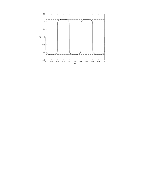
Figure 3: Filled curve: exact solution with $\tau-\tau_{0}=-0.07$, $K=5\pi$. Dashed lines: approximate bounds $y=\pm K[\tau_{0}-\tau]+(\ln 2)/K$.

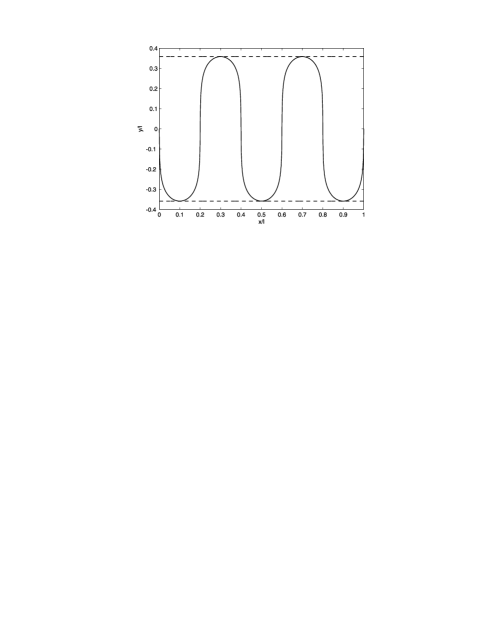
Figure 4: Filled curve: exact solution with $\tau-\tau_{0}=-0.02$, $K=5\pi$. Dashed lines: approximate bounds $y=\pm K[\tau_{0}-\tau]+(\ln 2)/K$.

When $K^{2}[\tau-\tau_{0}]$ is large and positive, the solution is smoother, approximated by a single sine wave,

$$Y=\pm\frac{\exp(-K^{2}[\tau-\tau_{0}])}{K}\sin(Kx)+O\left(\exp(-2K^{2}[\tau-\tau_{0}])\right),$$ (20)

whose amplitude decreases exponentially in time. This is the sinusoidal solution of the classical linear diffusion equation that approximates the curvature driven diffusion equation at large times in the small-slope approximation.

The number of extrema $n$ within the fixed domain $[0,1]$ may be freely chosen. For large values of the parameter $K^{2}\tau_{0}$, as in Fig. 3, the initial condition is described well as a periodic square wave, resembling a diffraction grating. The time scale for decay may be viewed as the time at which the formal expression (19) for $Y_{\max}$ is zero. This is

$$t=t_{0}+\frac{\ell^{2}\ln 2}{n^{2}\pi^{2}B}.$$

Fig. 3 evidences considerable smoothing of the initial conditions but at this time, the solution does not yet resemble a simple sinusoid. At larger times, the solution is close to a single sinusoidal wave. In the regime of the sinusoidal profile, from (20) decay times are shorter, of the order of the standard time $(\ell/n\pi)^{2}/B$ that is familiar from exponential decay of Fourier modes in linear diffusion models (e.g. [11]) when the half-wavelength $\ell/n$ is the typical distance between neighboring regions of high and low mass concentration.

4 Surface evolution by evaporation and condensation

For some metals such as gold, surface diffusion persists for several thousand years as the dominant surface transport mechanism but for others such as magnesium, after a time less than a day, surface evolution occurs predominantly by evaporation-condensation. As described by Mullins [25], the Gibbs–Thomson relation for evaporation rate in terms of deficit from equilibrium pressure over a curved surface, leads to a second-order equation for diffusion by mean curvature. In terms of two-dimensional Cartesian coordinates $(x,y)$ and time $t$, the Mullins equation for points on a material surface is

$$y_{t}=B\frac{y_{xx}}{1+y_{x}^{2}},$$

where $B$ is constant. This equation applies to two dimensional cross sections of solids when surface nano-scale features such as grooves, ridges and furrows extend rectilinearly into the third dimension. Because of the nonlinearity, very few useful exact solutions to this equation are known [9], except in a linear approximation. Two decades ago [6], the exact solution was constructed in parametric integral form for nonlinear surface evolution near a symmetric grain boundary, with constant slope at the grain boundary groove, initial flatness and zero displacement at infinity. A similar procedure produces the more general “open angle” solutions for deposition in a wedge [21]. Subsequently, the fourth-order Mullins equation for curvature-driven surface diffusion on an almost-isotropic material, was solved with boundary conditions representing a symmetric grain boundary [7, 29, 8].

In the context of surface evaporation, the parallel asymptotes of the grim reaper solution represent a long thin metallic foil that is evaporating at the ends. The constant travelling-wave speed of the grim reaper solution shows that evaporation will take place at a constant rate that depends on foil thickness as well as the evaporation coefficient $B$. The thickness $\Delta x$ is the distance between the two asymptotes, $\Delta x=\pi B/c$. Hence the steady evaporation rate at the end of a strip of metallic foil will be $c=\pi B/\Delta x$. For example, for a foil of a few microns in thickness made of the volatile metal Mg, this rate will be of the order of one millimetre per millenium.

In the context of metal surface smoothing, the periodic solution of the previous section predicts the smoothing of initial conditions that resemble a diffraction grating. For a surface fixed at two end-points, we prescribe the boundary conditions

$$y=0,\qquad x=0,\ell.$$

Physically, this corresponds to the surface being clamped and shielded from the surrounding atmosphere outside of the exposed spatial domain $[0,\ell]$.

4.1 Evaporation from anisotropic crystals

C. Herring [20], showed that for anisotropic crystals, surface energy is proportional to $b(\phi)(\gamma+\gamma^{\prime\prime}(\phi))$, where $\phi$ is the polar angle $\arctan y_{x}$, $\gamma$ is surface tension and $b$ is an evaporation coefficient. An equation of the form

$$y_{t}=D(y_{x})y_{xx},$$ (21)

implying the standard nonlinear diffusion equation (8) with $u=y_{x}$, may be regarded as an anisotropic form of the Mullins evaporation-condensation equation

$$y_{t}=B(y_{x})\frac{y_{xx}}{1+y_{x}^{2}},$$

with surface slope-dependent anisotropy factor $B(y_{x})=D(y_{x})(1+y_{x}^{2})$, which originates in the physical derivation from a constant multiple of $b(\phi)(\gamma+\gamma^{\prime\prime}(\phi))$ (e.g. [28]). Crystalline materials are indeed anisotropic, with the evaporation coefficient minimized when the cut surface is aligned with crystal planes. The group of equivalence transformations of this class of equations includes the general linear group $GL(2,{\mathbb{R}})$. By the polar decomposition theorem, each invertible linear transformation can be decomposed as an othogonal transformation followed by multiplication by a positive definite symmetric dilatation matrix. Under a rotation about the origin by angle $\alpha$,

$$\bar{x}=x\cos\alpha-y\sin\alpha,\qquad\bar{y}=x\sin\alpha+y\cos\alpha,\qquad\bar{t}=t,$$

$$\bar{u}=\bar{y}_{\bar{x}}=\frac{u+\tan\alpha}{1-u\tan\alpha},\qquad y_{x}=\frac{-\sin\alpha+\bar{y}_{\bar{x}}\cos\alpha}{\cos\alpha+\bar{y}_{\bar{x}}\sin\alpha},\qquad y_{xx}=\frac{\bar{y}_{\bar{x}\bar{x}}}{(\cos\alpha+\bar{y}_{\bar{x}}\sin\alpha)^{3}}.$$

The axis $\bar{x}=0$ has been rotated by angle $-\alpha/2$. Writing $\bar{\theta}=\arctan\bar{y}_{\bar{x}}$,

$$y_{t}=\frac{{\mathbf{n}}\cdot{\mathbf{e}}_{\bar{y}}}{{\mathbf{n}}\cdot{\mathbf{e}}_{y}}\bar{y}_{\bar{t}}=\frac{\cos\bar{\theta}}{\cos(\bar{\theta}-\alpha)}\bar{y}_{\bar{t}}=\frac{1}{\cos\alpha}\frac{1}{1+\bar{y}_{\bar{x}}\tan\alpha}\bar{y}_{\bar{t}}.$$

Hence, by rotation, the isotropic nonlinear diffusion equation (21) is equivalent to

$$\bar{y}_{\bar{t}}=\bar{D}(\bar{y}_{\bar{x}})\bar{y}_{\bar{x}\bar{x}},\qquad\bar{D}(s)=\frac{1}{(s\sin\alpha+\cos\alpha)^{2}}D\left(\frac{s\cos\alpha-\sin\alpha}{s\sin\alpha+\cos\alpha}\right).$$

Tritscher [27] used this device of rotational equivalence classes to solve integrable forms of fourth-order surface diffusion equations. In particular, after rotation by angle $\alpha=\pi/2$,

$$\bar{D}(\bar{y}_{\bar{x}})=\frac{1}{\bar{y}_{\bar{x}}^{2}}D\left(\frac{-1}{\bar{y}_{\bar{x}}}\right).$$

By following the $\pi/2$ rotation by a trivial reflection $\bar{x}\to-\bar{x}$, we recover the result of the reciprocal transformation (7).

By the principal axis theorem, a positive symmetric matrix can be written as $O^{t}QO$, where $O$ is a rotation matrix and $Q$ is diagonal, $Q_{i}^{j}=a_{i}\delta_{i}^{j}$ with $a_{j}>0$. Therefore, to consider the effect of an additional dilatation, we need only consider the effect of a diagonal rescaling:

$$\bar{x}=a_{1}x,\qquad\bar{y}=a_{2}y,\qquad\bar{y}_{t}=a_{1}^{2}D\left(\frac{a_{1}}{a_{2}}\bar{y}_{\bar{x}}\right)\bar{y}_{\bar{x}\bar{x}},$$

which although trivial, allows us to construct simple anisotropic models from the rotationally invariant isotropic model.

5 Anisotropic analogs of isotropic model solutions

The scale invariance group still applies to the general anisotropic diffusion equation (21). Therefore both expanding and shrinking types of similarity solution exist but they may be significantly different from those of the isotropic model. The grain boundary groove solution still exists, as can be seen from the solvability of the reduced boundary value problem on ${\mathbb{R}}^{+}\times{\mathbb{R}}^{+}$,

$$u=F(\rho),\qquad\rho=xt^{-1/2},$$

$$\frac{-\rho}{2}F^{\prime}(\rho)=\frac{d}{d\rho}[D(F)F^{\prime}(\rho)],$$

$$F(0)=m>0,\qquad F(\rho)\to 0,\qquad\rho\to\infty.$$

The grain-boundary groove solutions for all models have some common features. Although it represents a highly anisotropic material, the linear model groove solution approximates that of an isotropic model for groove slopes of up to 0.5, which was used in Mullins’ original paper [25]. However, whereas the linear model predicts that the groove depth increases in proportion to $m$, the groove depth increases very slowly, of order $(\log m)^{0.5}$ at large $m$ for the isotropic model [4].

5.1 Anisotropic homothetically shrinking closed curve

For anisotropic evaporating materials, the closed-curve homothetic solution represents the fixed-shape cross section of an evaporating wire, which is circular when the material is isotropic.

The homothetic evaporating closed-curve solution satisfies

$$y=[t_{0}-t]^{1/2}G(\rho),\qquad\rho=x[t_{0}-t]^{-1/2},$$

$$\frac{-G}{2}+\frac{\rho}{2}G^{\prime}(\rho)=G^{\prime\prime}(\rho)D(G^{\prime}),$$

$$G^{\prime}(0)=0,\qquad G(\rho_{0})=0,\qquad G^{\prime}(\rho)\to\infty,\qquad\rho\to\rho_{0}.$$

This implies

$$u=F(\rho),\qquad F=G^{\prime},$$

$$\frac{\rho}{2}F^{\prime}(\rho)-D^{\prime}(F)(F^{\prime})^{2}=F^{\prime\prime}(\rho)D(F),$$ (22)

$$F(0)=0,\qquad F(\rho)\to\infty,\qquad\rho\to\rho_{0}.$$

For some functions $D(u)$, the homothetic closed-curve solution does not exist. For example, with the linear model with constant $D$, the general solution satisfying $F(0)=0$ must be

$$F(\rho)=\frac{\sqrt{\pi}}{2}A\,\text{erf}\,(\rho)=A\int_{0}^{\rho}e^{-s^{2}/4}ds,\qquad A\in{\mathbb{R}}.$$

Since this cannot take an infinite value at any point $\rho=\rho_{0}\in{\mathbb{R}}$, the closed-curve homothetic solution does not exist.

Let us now assume that $F(\rho)\approx A_{0}(\rho_{0}-\rho)^{\nu}$. If a homothetic closed-curve solution exists, $G(\rho_{0})\in(-\infty,0)$, and

$$0=G(\rho_{0})=G(0)+\int_{0}^{\rho_{0}}F(s)ds.$$

This can hold only if the integral does not diverge, implying

$$-1<\nu<0.$$

Now we suppose that at large $u,D(u)$ is asymptotic to a power law $D(u)\approx D_{0}u^{n}$. Then by balancing terms at the leading order in $\rho_{0}-\rho$, (22) implies

1. $n=1/\nu$, which is less than $-1$, and $\rho_{0}=-2\nu D_{0}A_{0}^{1/\nu}$, or,

2. $n=\frac{1-\nu}{\nu}$, which is less than $-2$.

For the linear model, the anisotropy factor is $B(u)=(1+u^{2})D$ which diverges when the curve is vertical. In the current application, we are interested in cases of realistic anisotropy for which the evaporation coefficient and the anisotropy factor are bounded, and the latter with a minimum value greater than zero:

$$\forall\,u\in{\mathbb{R}},\qquad 0<B_{0}<B(u)<B_{\infty}<\infty.$$

That statement must be true, independent of the orientation of the coordinate axes. For example after rotation by $\pi/2$ it must be true that $\bar{D}(\bar{u})\to\bar{D}_{0}\in(0,\infty)$ as $\bar{u}\to 0$. By rotating back to the original orientation, this implies

$$D(u)=u^{-2}\bar{D}(u)\sim\bar{D}_{0}u^{-2}.$$

This physical restriction rules out scenario $(ii)$ in the above leading-order analysis. The simplest example satisfying the restriction is $D(u)=1/(1+(\beta u)^{2})$ ($\beta\in{\mathbb{R}}$ constant) for which the anisotropy factor $B(y_{x})$ varies between 1 and $\beta^{2}$. In this case the homothetic solution is simply an ellipse

$$\frac{x^{2}}{2[t_{0}-t]}+\frac{y^{2}}{2\beta^{2}[t_{0}-t]}=1$$

elongated in the direction of weakest evaporation.

5.2 Grim reaper solution for anisotropic material

The grim reaper solution is a travelling wave constrained between two vertical asymptotes. This implies a steady state solution of the equation $u_{t}=[D(u)u_{x}]_{x}$. For arbitrary $D(u)$, there exists a two-parameter steady state solution

$$u_{s}(x)=K^{-1}(cx+c_{2}),$$

where

$$K(u)=\int_{0}^{u}D(s)ds$$

which is an increasing invertible function because $D(s)>0$. This integrates formally to

$$y(x,t)=y_{0}(t)+\int_{0}^{x}u_{s}(x_{1},t)dx_{1}.$$

It then follows from (21) that $y_{0}(t)$ can only be a constant-velocity translation, $y_{0}=c(t-t_{0})$. This travelling wave solution does not necessarily have a vertical asymptote. For example, there is no such asymptote when $D$ is constant. However if $D(s)$ satisfies the physical requirement $D(s)\approx s^{-2}$, it follows that $K(u)$ has a finite limit as $u\to\infty$, therefore $K^{-1}$ has a vertical asymptote at some location $x=x_{0}$, duplicated at $x=-x_{0}$ if $D(s)$ is an even function, as is commonly the case when the $x$-axis denotes the orientation of the crystal planes from where evaporation is weakest.

6 Anisotropic models allowing functional separation

The classification of Doyle and Vassiliou gives all functions $D(s)$ for which functional separation of variables is possible in the general form

$$\bar{u}=f(u)=v(x)+w(t),$$ (23)

with $f$ an invertible function.

The simplest example of a physically feasible isotropic model is simply that obtained from the isotropic diffusion equation by unequally rescaling $x$ and $y$. For example, Fig. 2 could be dilated in one direction, displaying a non-homothetic closed curve approaching a homothetically shrinking ellipse.

The only other member of the Doyle–Vassiliou list with realistic anisotropy is much more complicated:

$$D(u)=D_{0}\cos(z(Au)),\qquad Au=\int_{0}^{z}(\cos s)^{-3/2}ds,\qquad-\pi/2<z<\pi/2.$$ (24)

This model is close to isotropic when $A=\sqrt{2}$. In that case, it is easy to show that when $u(=y_{x})$ is small, $B(u)=1+O(u^{4})$ and $B\to 2$ as $u\to\infty$. In Fig. 5, the function $D(u)/D_{0}$ for this weakly anisotropic model is compared to $D(u)/D_{0}$ of the isotropic model.

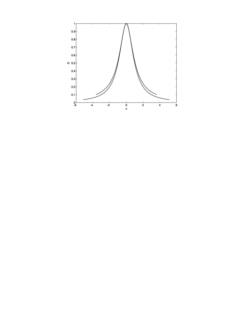
Figure 5: Nonlinear diffusivity function $D(u)$ for isotropic evaporation (lower) and anisotropic model (upper).

For the sake of completeness, we construct the special solution $u(x,t)$ compatible with (23), that was not given explicitly by Doyle and Vassiliou [15]. The parameter $A$ may be changed by rescaling $u$. For convenience, without loss of generality we now set $A$ to 1. Also we may set $D_{0}$ to 1 by using $D_{0}t$ as the time coordinate. From the general approach of Doyle and Vassiliou [15], $\bar{u}$ is a sum of separated functions $v(x)$ and $w(t)$ satisfying

$$v^{\prime\prime\prime}(x)+\frac{1}{2}[v^{\prime}(x)]^{3}=0,$$ (25)

$$w^{\prime}(t)=W(w)=\cos w\left[v^{\prime\prime}\cos v+\frac{1}{2}(v^{\prime})^{2}\sin v\right]+\sin w\left[-v^{\prime\prime}\sin v+\frac{1}{2}(v^{\prime})^{2}\cos v\right].$$

By construction, the following are first integrals of (25), which can be verified by substitution:

$$\lambda=v^{\prime\prime}(x)\cos v+\frac{1}{2}(v^{\prime})^{2}\sin v,\qquad\mu=-v^{\prime\prime}(x)\sin v+\frac{1}{2}(v^{\prime})^{2}\cos v.$$

It then follows that $w^{\prime}(t)=\lambda\cos w+\mu\sin w$, and that

$$t=\frac{2}{R^{2}}\int\frac{dw}{\sin(w+\delta)},\qquad x=\frac{1}{R}\int_{0}^{v}\frac{ds}{\sqrt{\cos(s-\delta)}},$$ (26)

with constants $x_{0}$, $t_{0}$, $R=\pm 2^{1/2}(\mu^{2}+\lambda^{2})^{1/4}$ and $\delta=\arctan(\lambda/\mu)$, whose arbitrariness is of little consequence. Let $v^{\prime}(x)=W(v)$, so $v^{\prime\prime}(x)=WW^{\prime}(v)$. Then

$$WW^{\prime}(v)\cos v+\frac{1}{2}W^{2}\sin v=\lambda,\qquad-WW^{\prime}(v)\sin v+\frac{1}{2}W^{2}\cos v=\mu$$

$$\Rightarrow\quad-\lambda\tan v+\frac{1}{2}W^{2}\frac{\sin^{2}v}{\cos v}+\frac{1}{2}W^{2}\cos v=\mu$$

$$\Rightarrow\quad W^{2}=2(\mu\cos v+\lambda\sin v)=R^{2}\cos(v-\delta)\quad\Rightarrow\quad v^{\prime}(x)=\pm R\sqrt{\cos(v-\delta)},$$

$$x=\frac{1}{R}\int_{0}^{v}\frac{ds}{\sqrt{\cos(s-\delta)}}.$$

When we include the parameter $B_{0}$, the general solution for $v$ and $w$ in terms of elementary functions, the standard elliptic integral $F(\theta|\frac{1}{2})$ and the standard Jacobi elliptic function $\text{sn}(X|\frac{1}{2})$, is

$$w=2\arctan e^{R^{2}B_{0}t/2}-\delta\qquad\mbox{and}\qquad v=2\arcsin\left(\frac{1}{\sqrt{2}}\,\text{sn}\left(\frac{R[x-x_{0}]}{\sqrt{2}}\Big{|}\frac{1}{2}\right)\right)+\delta,$$

where

$$x_{0}=\frac{\sqrt{2}}{R}F\left(\arcsin\left(\sqrt{2}\sin\frac{\delta}{2}\right)\Big{|}\frac{1}{2}\right).$$

Since $u$ is a function of $w(t)+v(x)$, we see that the choice of parameters $R$ and $\delta$ has little consequence on the form of the solution $u(x,t)$. A shift in the phase variable $\delta$ has the effect of a translation in $x$ by $x_{0}(\delta,R)$. A change of amplitude $R$ has the effect of rescaling $x$ and $t$ to $Rx$ and $R^{2}t$.

Modulo a time-dependent vertical translation, the curve $y(x,t)$ is obtained from $u(x,t)$ by integration. Since the integrands in (24) and (26) must be real valued, the constructed solution has a truncated domain. An example is given in Figs. 6–8.

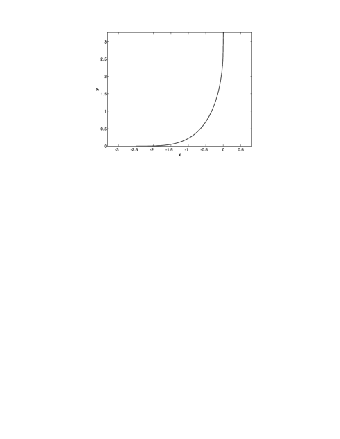
Figure 6: Portion of solution curve for anisotropic model with $R=1$ and $\delta=0$, at $t=0$.

As $t$ approaches $-\infty$, the solution approaches a steady state. Since $D(u)$ is symmetric, this steady state is a symmetric grim reaper. It is approximated in Fig. 8 by taking $t=-8.0$.

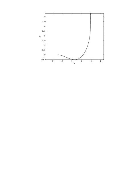
Figure 7: Portion of solution curve for anisotropic model at $t=-2.0$.

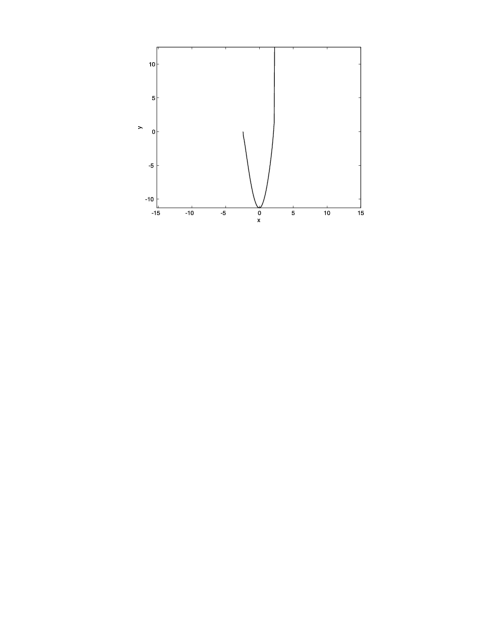
Figure 8: Portion of solution curve for anisotropic model at $t=-8.0$.

The curve is not symmetric, as can be seen in Fig. 7. This asymmetry causes its domain to shift slightly from right to left. For $t\leq 0$, the curve has a vertical asymptote at moving location

$$x=x_{u}=\int_{0}^{\pi/2-w(t)}(\cos s)^{-1/2}ds$$

and a local minimum at

$$x=x_{\ell}=-\int_{0}^{w(t)}(\cos s)^{-1/2}ds.$$

7 Conclusion

Of the exact solutions to the curve shortening equation known to us, most can be obtained by Lie point symmetry reductions. The two interesting solutions that cannot be constructed in this way, can indeed be recovered by functional separation of variables for the standard nonlinear diffusion equation (3) that is obtained from the curve shortening equation by differentiation. The classification obtained by Doyle and Vassiliou [15] of nonlinear diffusion equations that admit functional separation of variables, leads to the two exact non-self-similar solutions with non-trivial initial conditions that appear to be achievable in an approximate sense in applications. In addition, it leads to a new separated solution for a physically realistic anisotropic evaporation-condensation diffusion equation. Although the second order nonlinear surface evolution equations for slope $u(x,t)$ ($\equiv y_{x}(x,t)$ admit a number of possibilities for functional separation of variables in Cartesian coordinates, we have proved that this is not possible for the equation (2) governing $y(x,t)$, nor is it possible in a coordinate system consisting of canonical variables for a symmetry other than translation. This is in contrast with the point symmetry analysis, which leads to a richer array of possibilities for the evolution of $y(x,t)$ than for the evolution of $u(x,t)$.

The invariance of the isotropic equation (10) under the well known reciprocal transformation was shown (Proposition 2.1) to lead to no new planar curve heat flows. The group of geometric equivalence transformations of the class of general anisotropic equations (21) includes not only the reciprocal transformation in the guise of a reflection in the plane, but the whole general linear group. The equivalence is shown by carrying out the equivalence transformations explicitly. Physical evaporation coefficients must have a positive real value when the surface is oriented along the crystal planes. Since physical restrictions must be independent of orientation of the coordinate axes, it follows from the equivalence transformations that the nonlinear diffusivity $D(y_{x})$ must behave like $y_{x}^{-2}$ at large-slope. This also allows for the existence of a closed non-circular homothetic solution which cannot exist unless $D(u)$ decreases faster than $u^{-1}$. The Doyle–Vassiliou classification produces another anisotropic model that satisfies this physical requirement. An exact solution has been constructed, involving Jacobi elliptic functions and other inverse integrals of rational functions.

Exact solutions sometimes have the advantage of leading to concise conceptually simple relationships. For example, Fig. 3 demonstrates the efficacy of a simple expression for wave amplitude of a corrugated nano-scale surface in the early stages of smoothing by evaporation-condensation when the system cannot be adequately described by a linear model. However, exact solutions can be obtained only in very special cases of initial and boundary conditions, so that approximate numerical solution methods will continue to be important.

Acknowledgements

This paper is submitted in appreciation of the valuable on-going contributions of Professor Willard Miller Jr. The first author gratefully acknowledges support by the Australian Research Council under project DP1095044.

References

- [1]
- [2] Abresch U., Langer J. The normalized curve shortening flow and homothetic solutions, J. Differential Geom. 23 (1986), 175–196.
- [3] Angenent S., On the formation of singularities in the curve shortening flow, J. Differential Geom. 33 (1991), 601–633.
- [4] Arrigo D.J., Broadbridge P., Tritscher P., Karciga Y., The depth of a steep evaporating grain boundary groove: application of comparison theorems, Math. Comput. Modelling 25 (1997), no. 10, 1–8.
- [5] Bluman G.W., Reid G.J., Kumei S., New classes of symmetries for partial differential equations, J. Math. Phys. 29 (1988), 806–811, Erratum, J. Math. Phys. 29 (1988), 2320.
- [6] Broadbridge P., Exact solvability of the Mullins nonlinear diffusion model of groove development, J. Math. Phys. 30 (1989), 1648–1651.
- [7] Broadbridge P., Tritscher P., An integrable fourth-order nonlinear evolution equation applied to thermal grooving of metal surfaces, IMA J. Appl. Math. 53 (1994), 249–265.
- [8] Broadbridge P., Goard J.M., Temperature-dependent surface diffusion near a grain boundary, J. Engrg. Math. 66 (2010), 87–102.
- [9] Cahn J.W., Taylor J.E., Overview no. 113 surface motion by surface diffusion, Acta Metall. Mater. 42 (1994), 1045–1063.
- [10] Cao F., Geometric curve evolution and image processing, Lecture Notes in Mathematics, Vol. 1805, Springer-Verlag, Berlin, 2003.
- [11] Carslaw H.S., Jaeger J.C. Conduction of heat in solids, 2nd. ed., Clarendon Press, Oxford, 1959.
- [12] Chou K.-S., Li G.-X., Optimal systems and invariant solutions for the curve shortening problem, Comm. Anal. Geom. 10 (2002), 241–274.
- [13] Clarkson P.A., Fokas A.S., Ablowitz M.J., Hodograph transformations of linearizable partial differential equations, SIAM J. Appl. Math. 49 (1989), 1188–1209.
- [14] Daskalopoulos P., Hamilton R., Sesum N., Classification of compact ancient solutions to the curve shortening flow, J. Differential Geom. 84 (2010), 455–465, arXiv:0806.1757.
- [15] Doyle P.W., Vassiliou P.J., Separation of variables for the 1-dimensional non-linear diffusion equation, Internat. J. Non-Linear Mech. 33 (1998), 315–326.
- [16] Galaktionov V.A., Dorodnitsyn V.A., Elenin G.G., Kurdyumov S.P., Samarskii A.A., A quasilinear equation of heat conduction with a source: peaking, localization, symmetry, exact solutions, asymptotic behavior, structures, J. Soviet Math. 41 (1988), 1222–1292.
- [17] Gage M., Hamilton R., The heat equation shrinking convex plane curves, J. Differential Geom. 23 (1986), 69–96.
- [18] Grayson M. 1987 The heat equation shrinks embedded plane curves to round points, J. Differential Geom. 26 (1987), 285–314.
- [19] Halldorsson H.P., Self-similar solutions to the curve shortening flow, arXiv:1007.1617.
- [20] Herring C., Surface tension as a motivation for sintering, in The Physics of Powder Metallurgy, Editor W.E. Kingston, McGraw-Hill, 1951, 143–179.
- [21] Ishimura N., Curvature evolution of plane curves with prescribed opening angle, Bull. Austral. Math. Soc. 52 (1995), 287–296.
- [22] King J.R., Emerging areas of mathematical modelling, R. Soc. Lond. Philos. Trans. Ser. A Math. Phys. Eng. Sci. 358 (2000), no. 1765, 3–19.
- [23] Kingston J.G., Rogers C., Reciprocal Bäcklund transformations of conservation laws, Phys. Lett. A 92 (1982), 261–264.
- [24] Malladi R., Sethian J.A., Image processing via level set curvature flow, Proc. Nat. Acad. Sci. USA 92 (1995), 7046–7050.
- [25] Mullins W.W., Theory of thermal grooving, J. Appl. Phys. 28 (1957), 333–339.
- [26] Olver P.J., Sapiro G., Tannenbaum A., Invariant geometric evolutions of surfaces and volumetric smoothing, SIAM J. Appl. Math. 57 (1997), 176–194.
- [27] Tritscher P., Integrable nonlinear evolution equations applied to solidification and surface redistribution, PhD Thesis, University of Wollongong, 1995.
- [28] Tritscher P., An integrable fourth-order nonlinear evolution equation applied to surface redistribution due to capillarity, J. Austral. Math. Soc. Ser. B 38 (1997), 518–541.
- [29] Tritscher P., Broadbridge P., Grain boundary grooving by surface diffusion: an analytic nonlinear model for a symmetric groove, Proc. Roy. Soc. Lond. A 450 (1995), no. 1940, 569–587.