Robustness of Prediction Based Delay Compensation for Nonlinear Systems

Abstract

Control of systems where the information between the controller, actuator, and sensor can be lost or delayed can be challenging with respect to stability and performance. One way to overcome the resulting problems is the use of prediction based compensation schemes. Instead of a single input, a sequence of (predicted) future controls is submitted and implemented at the actuator. If suitable, so-called prediction consistent compensation and control schemes, such as certain predictive control approaches, are used, stability of the closed loop in the presence of delays and packet losses can be guaranteed. In this paper, we show that control schemes employing prediction based delay compensation approaches do posses inherent robustness properties. Specifically, if the nominal closed loop system without delay compensation is ISS with respect to perturbation and measurement errors, then the closed loop system employing prediction based delay compensation techniques is robustly stable. We analyze the influence of the prediction horizon on the robustness gains and illustrate the results in simulation.

1 Introduction

In many of today’s control systems, delays and information losses between the controller, actuator, and sensor are often unavoidable. Such delays and dropouts must be accounted for during the controller design and the closed loop system analysis to avoid instability or performance decay. There are many causes for delays and information losses: often controller, sensors, and actuators are connected via a communication network. These kinds of systems are typically denoted as networked control systems, see Hespanha et al. (2007). For networked control systems delays and information losses might be due to network overload, long communication distances, routing, or hardware failure. Other sources might be long computation times, e.g. due to image processing, or solution of complex optimization problem, as in the case of predictive control. In other applications, delays and potential losses might be inherent to the problem under investigation. For instance, in some processes it is necessary to “charge” batteries before being able to collect a measurement or human interaction could be required to take measurements or apply new inputs.
By now, a series of approaches for the control of systems that are subject to delays and information losses exist. In particular, ideas based on Model Predictive Control (MPC) have demonstrated to be effective in dealing with both delays and information losses, see e.g. Findeisen and Allgöwer (2004); Findeisen (2006); Findeisen and Varutti (2009); Varutti et al. (2009); Grüne et al. (2009); Polushin et al. (2008); Lunze and Lehmann (2010); Bemporad (1998). Many of these approaches are based on the idea of compensating the unknown delays by sending not only one control action to the actuator, rather a complete input sequence (discrete time systems) or an input signal (continuous time systems), are submitted, where the signals sent are time-stamped. The actuator itself can then continue applying the old input until new data arrive or the input has been implemented. While suitable design of such a scheme often leads to nominal closed loop stability, only minor results with respect to robust stability are available.
In this work, we establish robust stability properties of so called prediction consistent delay compensation schemes, see Findeisen and Varutti (2009) and Varutti and Findeisen (2009) for the continuous time formulations and Grüne et al. (2009) for the discrete time case. Prediction consistent delay compensation schemes counteract the delays by submitting a complete consistent input trajectory (in the sense of a predicted behavior of the closed loop) to the actuator. Approaches following similar ideas, which, however, are only able to handle delays either on the sensor or actuator side, have been for example introduced in Bemporad (1998); Polushin et al. (2008) (see also Grüne et al. (2009) for a comparison).
Specifically, we establish that prediction consistent delay compensation schemes for discrete time nonlinear systems do admit, under certain conditions, inherent robustness. Precisely, if the nominal closed loop system without delays is input-to-state stable (ISS), cf. Sontag (2000), then the closed loop system subject to delays and utilizing a prediction consistent delay compensation approach is robustly stable. Additionally, we explicitly analyze the influence of the prediction horizon on the robustness gains and illustrate the results by a numerical simulation. The derived results significantly expand the applicability of prediction consistent delay compensation approaches, since they establish that these methods are also well suited for the robust case. It is important to stress that ISS results for predictive control methods are well established by now, refer to Magni and Scattolini (2007); Limon et al. (2009). Results with respect to ISS, delays, and predictive control approaches are, however, very limited. Exceptions are the results presented in Zavala and Biegler (2009), which, however, do not apply a compensation approach and thus can only derive ISS properties with respect to small delays. Similar results with respect to practical stability subject to delays have been presented in Findeisen (2006). Furthermore, recently stochastic stability properties of predictive control approaches over unreliable networks have been derived in Quevedo et al. (2011). These results, however, only hold for delays and losses of information on the actuator side.

2 Prediction Consistency: Setting and Nominal Results

In this paper, we consider discrete time nonlinear systems

$$x(n+1)=f(x(n),u(n),w(n)),$$ (1)

where $x\!\in\!X\!\subseteq\!\mathbb{R}^{n}$, $u\!\in\!U\!\subseteq\!\mathbb{R}^{m}$, and $w\!\in\!W$ represent respectively the state, the input and the disturbance/perturbation acting on the system, taken from the sets $X$, $U$, and $W$. In the following, for any time $n>n_{0}$, we denote with $x(n,n_{0},x_{0},u,w)$ the solution of (1) with initial time $n_{0}$, initial value $x_{n_{0}}$, input sequences $u$ and perturbation $w$, obtained by iterating (1) for $n_{0},\ldots,n$.

Remark 2.1

The disturbance $w$ can account for various uncertainties such as measurement uncertainties, disturbances on the input side, or model uncertainties.

Prediction consistent compensation:
We consider that the controller interacts with the sensors and actuators as shown in Figure 1. The implementation of the controller follows the ideas presented in Grüne et al. (2009) for discrete time systems and in Varutti and Findeisen (2009) for the continuous time case. A key component of all these approaches is a prediction algorithm, which makes use of a model of the system to deal with delays and information losses by forward predicting the (closed loop) plant and generating an input sequence which is communicated to the actuator.

For the prediction, a model of the plant is required. Our scheme relies on an approximating map $\tilde{f}(\cdot)$ of the nominal unperturbed system map $f(\cdot)$ in the sense that

$$\tilde{f}(x,u)\approx f(x,u,0).$$ (2)

The detailed approximation properties of $\tilde{f}(\cdot)$ are elaborated in Assumption 3.1(i), below. For instance, if $f(\cdot)$ is a discrete time model of a zero order hold sampled continuous time control system, then $\tilde{f}(\cdot)$ might be chosen as the numerical solution of the underlying differential equation over one sampling period with constant control value. Analogously to the plant, $\tilde{x}(n,n_{0},\tilde{x}_{n_{0}},\tilde{u})$ denotes the predicted solutions obtained by iterating

$$\tilde{x}(n+1)=\tilde{f}(\tilde{x}(n),\tilde{u}(n))$$ (3)

from $n_{0}$ to $n$ starting with initial value $\tilde{x}_{n_{0}}$ using $\tilde{u}$.
This prediction map is used by the controller to “forecast” the future system states based on past measurements. To infer properties of the closed loop from these forecast predictions, the real system state should coincide, or at least be close to the predicted state. A key requirement for the prediction $\tilde{x}$ to assume the same value as the real system state $x$ is that the control sequence $\tilde{u}$ used for the prediction coincides with the control sequence $u$ applied at the plant. In other words, we require the compensation algorithm to be prediction consistent, or, more formally:

Definition 2.2

(Prediction Consistency):
A prediction based delay compensation control scheme is called prediction consistent if at each time $n\in\mathbb{N}_{0}$ the identity $\tilde{u}(k)=u(k)$ holds for all $k\in\{0,\ldots,n\}$.

Note that the schemes proposed in Bemporad (1998); Grüne et al. (2009); Polushin et al. (2008) are prediction consistent in the sense of this definition.
Before describing in detail the scheme used, we introduce the following quantities and assumptions on the delays and information losses.

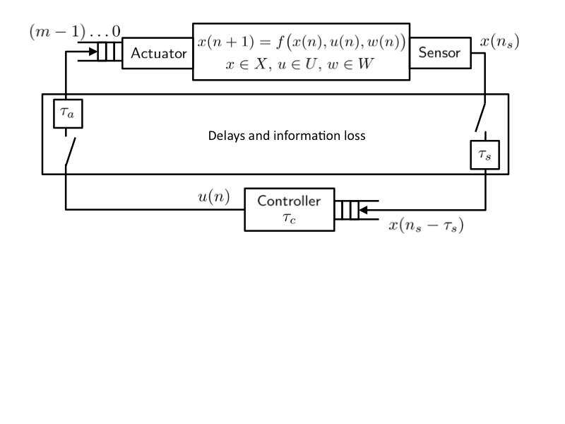
Figure 1: Sketch of the problem under investigation.

We refer with $n_{s}$, $n_{c}$, and $n_{a}$ to the time at the sensor, controller and actuator side respectively; $\tau_{s}$, and $\tau_{a}$ indicate the delays in the measurement and actuation channel, while $\tau_{c}$ represents potential computational delays; all delays are assumed to be bounded. Note, however, that the delays are not assumed to be constant, they can vary with time. Both measurements and input sequences can be lost and all the components — controller, sensor, and actuator — are supposed to have synchronized clocks. All measurements are time-stamped with the time instant $n_{s}$ from which they are collected, whereas the input is time-stamped with the value $n$ in which it is supposed to be applied to the system.The disordered arrival of packets is solved by taking the one with the most recent time-stamp. Additionally, the actuator is equipped with a buffer of length $m>1$.

To counteract and compensate delays and information losses, we propose the following scheme:

1. At each time $n_{c}$ the controller computes the predicted state $\tilde{x}(n)=\tilde{x}(n,n_{s},x(n_{s}),\tilde{u})$ at time $n$ (specified in Step (ii)) from the delayed measurement $x(n_{s})$ taken at time $n_{s}$ using the prediction control input $\tilde{u}$.

2. Based on the prediction $\tilde{x}(n)$, and the buffer length $m$, the controller computes an input sequence

   $$\mu(\tilde{x}(n),0),\ldots,\mu(\tilde{x}(n),m-1)$$ (4)

   which is sent to the actuator. This allows to have “backup” control values whenever transmission failures in the input or long delays occur.The prediction time $n$ is chosen such that the input sequence reaches the actuator in time. More precisely, for the prediction performed at time $n_{c}$, using an upper bound $\tau^{\max}\geq\tau_{a}+\tau_{c}$ we predict the future state for time $n=n_{c}+\tau^{\max}>n_{c}$ from the most recent available measurement taken at time $n_{s}\leq n_{c}$. The resulting input sequence is time-stamped with $n$ and sent to the actuator. The value $\tau(n):=n-n_{s}$ denotes the length of the resulting prediction interval.

3. The actuator buffers the input sequences and uses the most recent available one in its buffer to determine the control value applied to the plant.

Different approaches to generate prediction consistent input sequences can be employed, as long as they satisfy the prediction consistency condition stated in Definition 2.2. Without loss of generality, to generate the control sequence (4) of Step (ii) we consider two different approaches: generation by forward predicting a stabilizing static feedback, and by using predictive control schemes. Notice that it is possible to compute these sequences in many other ways, cf. Grüne et al. (2009); Varutti and Findeisen (2009); Polushin et al. (2008). All these approaches can be analyzed with the framework proposed in this paper.
Prediction consistent input generators:

• Static state feedback: the input sequence can be based on a static state feedback controller $K:X\to U$. In this case, from the predicted state $\tilde{x}(n)\in X$ we inductively compute

  $$\begin{array}[]{c}\tilde{x}(p+1)=\tilde{f}(\tilde{x}(p),K(\tilde{x}(p))),\\ p=n,\ldots,n+m-2,\end{array}$$ (5)

  and set

  $$\mu(\tilde{x}(n),q):=K(\tilde{x}(q)),\quad q=0,\ldots,m-1.$$ (6)

  For notation simplicity, although this is in general not required, we assume that the predictor (5) coincides with the one specified in Step (i). If we extend the prediction control sequence $\tilde{u}$ used in Step (i) for computing $\tilde{x}(n)$ by setting $\tilde{u}(n+q)=K(\tilde{x}(q))$, $q=0,\ldots,m-1$, then from (5),

  $$\begin{array}[]{c}\tilde{x}(p)=\tilde{x}(p,n_{s},x(n_{s}),\tilde{u}),\\ p=n,\ldots,n+m-2,\end{array}$$ (7)

  where $n_{s}=n-\tau(n)$ is the measurement time from Step (i).

• predictive control: If the controller is computed by a predictive control approach (MPC), then for a given initial value $x_{0}$ the MPC algorithm generates a finite horizon control sequence $u_{x_{0}}(0),\ldots,u_{x_{0}}(m-1)$. These control values are determined via an internal prediction inside the optimization algorithm starting from $x_{0}=\tilde{x}(n)$. This results in the predicted optimal trajectory

  $$\begin{array}[]{c}\tilde{x}(p)=\tilde{x}(p,n,\tilde{x}(n),u_{\tilde{x}(n)}),\\ p=n+1,\ldots,n+m-2.\end{array}$$ (8)

  For simplicity of exposition we assume that (3) is used to compute the internal prediction. While in a usual MPC scheme one would only use the first element of the optimal control sequence for feedback, in order to obtain the sequence (4), we set

  $$\mu(\tilde{x}(n),q)=u_{\tilde{x}(n)}(q),\quad q=0,\ldots,m-1.$$ (9)

  Again we can write $\tilde{x}(p)$ in the form (7) if we appropriately extend the prediction control sequence used in Step (i). Here we need to use $\tilde{u}(n+q)=u_{\tilde{x}(n)}(q)$, $q=0,\ldots,m-1$.

Both control approaches have certain advantages and disadvantages. Usage of a known static feedback law allows, in general, fast generation of input sequences. However, it might be difficult to take constraints or cost functions to be optimized into account. Obtaining a prediction consistent input sequence by MPC might be computationally challenging, however, it allows to directly consider constraints.

Overall closed loop system:
By $\sigma_{i}$, $i\in\mathbb{N}_{0}$, we denote in the following the times — numbered in increasing order — at which the actuator switches to a new control sequence, i.e., the times at which a control value $\mu(\tilde{x}(\sigma_{i}),0)$ is applied at the actuator. Henceforth, we will refer to the times $\sigma_{i}$ as the switching times. Using this, we can write the closed loop as

$$x(n+1)=f(x(n),\mu(\tilde{x}(\sigma_{i}),n-\sigma_{i}),w(n)),$$ (10)

for all $n\in\{\sigma_{i},\sigma_{i+1}-1\}$, where $\tilde{x}(\sigma_{i})=\tilde{x}(\sigma_{i},\sigma_{i}-\tau(\sigma_{i}),x(\sigma_{i}-\tau(\sigma_{i})),\tilde{u})$, and $\tau(n)=n-n_{s}$. The prediction consistency condition can now be ensured by suitable algorithms which enable controller and actuator to identify and correct prediction inconsistencies by means of sending time-stamped information. For more details see Grüne et al. (2009) and Varutti and Findeisen (2009). If prediction consistency holds, then from (10) it follows that

$$u(n)=\mu(\tilde{x}(\sigma_{i},\sigma_{i}-\tau(\sigma_{i}),x(\sigma_{i}-\tau(\sigma_{i})),\tilde{u}),n-\sigma_{i})$$ (11)

for all $n\in\{\sigma_{i},\sigma_{i+1}-1\}$ and all $i=0,1,2,\ldots$.

In order to simplify the analysis, we shift our “time” and number the $\sigma_{i}$ such that $\sigma_{0}=0$. The resulting closed loop trajectory for $n\geq 0$ is uniquely determined by the value $x_{0}=x(0)$, the switching times $\sigma_{i}$ and the delays $\tau(\sigma_{i})$. We denote this closed loop trajectory by $x_{cl}(n,x_{0},\sigma_{\cdot},\tau,w)$ and use the brief notation $x_{cl}(n)$.

Remark 2.3

(Open loop prediction versus closed loop)
The closed loop system (10) appears to depend only on the predictions $\tilde{x}(\sigma_{i},\sigma_{i}-\tau(\sigma_{i}),x(\sigma_{i}-\tau(\sigma_{i})),\tilde{u}))$ for the switching times $\sigma_{i}$. However, in the Steps (iia) and (iib), above, also the predictions $\tilde{x}(p)$ for all remaining times $p\neq\sigma_{i}$ are needed. Note that each $p$ appears in (iia) or (iib) for several different $n$ and thus at different times/runs of these steps different values $\tilde{x}(p)$ are computed for one and the same $p$. In (iia) only one of them, more precisely the one corresponding to the maximal $n$ satisfying $n=\sigma_{i}$ for some $i$, is actually used in order to compute the control value $u(n)$ applied to the closed loop system. Hence, for each closed loop trajectory $x_{cl}(\cdot)$ and each time $n\geq 0$, there is a unique prediction $\tilde{x}(n)$ which is used either explicitly for $n=\sigma_{i}$ in (10) or implicitly for $n=p$ in Step (iia) in order to compute the value $u(n)$ eventually applied to the system.We denote this predicted state by $\tilde{x}_{cl}(n)$.
In (iib), since the optimizations are carried out over the whole prediction horizon, for each computation all predicted values (also those for $k>n$) affect the computed control sequence. Since these future predictions are uniquely determined by $\tilde{x}_{cl}(n)$ and (3), we do not denote them explicitly.

In the next section we establish the main result, namely robust stability and the influence of the prediction horizon on the robustness gains of the proposed scheme.

3 Stability and robustness

The main idea of our analysis is to replace the closed loop system (10) by a non-delayed system in which the prediction errors due to the delay effects are captured as measurement errors. This fundamentally differs from other stability analysis methods for delayed systems in which the delay is explicitly taken into account. While our method may lead to more conservative results, its main advantage is the fact that it is applicable to general nonlinear systems under rather mild conditions.

Bounding the influence of prediction errors:
To capture the prediction errors via measurement errors, we need the following additional assumptions with respect to the estimates on the prediction accuracy and the sensitivity of the solution with respect to $w$.

Assumption 3.1

(Prediction error and perturbations)
(i) The prediction error for the nominal system satisfies

$$\|\tilde{x}(n,n_{0},\tilde{x}_{0},u)-x(n,n_{0},x_{0},u,0)\|\leq\varepsilon(n-n_{0},\|\tilde{x}_{0}-x_{0}\|)$$

for all $x_{0},x_{1}\in X$ and all $u\in U$, where $\varepsilon:(\mathbb{R}_{0}^{+})^{2}\to\mathbb{R}_{0}^{+}$ is a monotonically increasing, continuous function in both arguments.
(ii) The influence of the perturbation can be bounded by

$$\|x(n,n_{0},x_{0},u,0)-x(n,n_{0},x_{0},u,w)\|\leq\eta(n-n_{0},\|w\|_{\infty})$$

for all $x_{0}\in X$ and all $u\in U$; $\eta:(\mathbb{R}_{0}^{+})^{2}\to\mathbb{R}_{0}^{+}$ is a continuous function which is monotonically increasing in its first argument and satisfies $\eta(n,\cdot)\in{\mathcal{K}}$ for all $n\geq 0$. In particular, $\eta(n,w)=0$ for all $n\in\mathbb{N}_{0}$ if $w\equiv 0$.

If required, explicit expressions for $\varepsilon$ and $\eta$ can be derived from suitable properties for $f(\cdot)$ and $\tilde{f}(\cdot)$. For example, if $\tilde{f}(\cdot)$ is a numerical approximation (e.g. for a continuous time system) with convergence order $p\in\mathbb{N}$ which is Lipschitz in $x$ with Lipschitz constant $L$, then a standard error estimation from numerical analysis yields

$$\varepsilon(k,r)=(e^{Lk}-1)Kh^{p}+e^{Lk}r,$$ (12)

where $h$ is the (fixed) time step used in the numerical scheme and $K$ is a suitable constant. Alternatively, a numerical step size controlled scheme could be used. In this case the term $Kh^{p}$ in (12) is replaced by a user specified desired accuracy $\hat{\varepsilon}$.

If $f$ is Lipschitz in $x$ with constant $L$ and satisfies

$$\|f(x,u,w)-f(x,u,0)\|\leq\rho(\|w\|)$$

for some ${\mathcal{K}}_{\infty}$-function $\rho$, then

$$\eta(k,r)=(e^{Lk}-1)\rho(r)/L$$ (13)

holds.

Remark 3.1

(Open loop stable and unstable systems)
Note that the exponential growth of the error terms in $k$ in (12) and (13) is a worst case estimate which applies if the plant is open loop unstable. If we assume that the system to be controlled is open loop stable for $w\equiv 0$ (e.g. if the plant is pre-stabilized by a feedback controller situated at the plant), then one only has linear, not exponential growth of the error terms in $k$.

Non-delayed closed loop system:
The auxiliary system we use for the analysis is given by

$$x(n+1)=f(x(n),\mu(x(\sigma_{i})+v(\sigma_{i})),n-\sigma_{i}),w(n))$$ (14)

for $n\in\{\sigma_{i},\sigma_{i+1}-1\}$ and all $i\in\mathbb{N}_{0}$. The solution, which depends on the initial value $x_{0}$, the perturbation functions $w(\cdot)$ and $v(\cdot)$ and the switching sequence $\sigma_{i}$, is denoted by $x_{a}(n,x_{0},v,w)$.

Observe that (10) and (14) coincide for

$$v(\sigma_{i}):=\tilde{x}_{cl}(\sigma_{i})-x(\sigma_{i}),\quad i=0,1,2,\ldots$$

for $\tilde{x}_{cl}$ from Remark 2.3. Similarly, we define

$$v(n):=\tilde{x}_{cl}(n)-x_{a}(n,x_{0},v,w),\quad n\neq\sigma_{i}.$$ (15)

Note that in contrast to $v(\sigma_{i})$, $i=0,1,2,\ldots$, which are values we are free to choose in (14), the values in (15) are determined by the dynamics of the system and the predictor.

The key requirement to establish robustness of the closed loop is now to assume that the auxiliary system is ISS with respect to $v$ and $w$.

Assumption 3.2

(ISS of the auxiliary system)
We assume that the system (14) is ISS with respect to perturbations and measurement errors, i.e. there exist $\beta\in{\mathcal{K}}{\mathcal{L}}$ and $\gamma_{w}$, $\gamma_{v}\in{\mathcal{K}}_{\infty}$ such that

$$\|x_{a}(n,x_{0},v,w)\|\leq\max\{\beta(\|x_{0}\|,n),\gamma_{w}(\|w\|_{\infty}),\gamma_{v}(\|v\|_{\infty})\}$$

holds for each initial value $x_{0}$, each sequence $(\sigma_{i})_{i\in\mathbb{N}_{0}}$ satisfying $0\leq\sigma_{i+1}-\sigma_{i}\leq m$, each perturbation function $w\in W$ and each measurement error satisfying (15).

Note that for simplicity of exposition we work with a global ISS assumption. All subsequent statements can be modified in a straightforward way if ISS only holds for sufficiently small perturbations and for initial values in a bounded subset of the state space.

Remark 3.2

(ISS of the auxiliary system and MPC)
For the MPC setting in Case (iib), Assumption 3.2 may be optimistic even for $w\equiv 0$ and $v\equiv 0$, since the controller is computed from an optimization over the approximate prediction (3) instead of optimizing over the exact solution of the (nominal) exact system (1). Hence, in general, we can only expect stability for the closed loop approximate model rather than for the exact one. For simplicity of exposition, we work with the simplified assumption that the MPC controller stabilizes the exact model (1). If desired, this additional error source could be rigorously taken into account in the subsequent analysis by formulating Assumption 3.2 for an appropriately perturbed version of the closed loop approximate system (3). Approaches in this direction can be found, for example, in Grüne and Nešić (2003); Elaiw (2007). These references also show how the needed robustness of the MPC controller (and more general optimization based controllers) can be obtained from regularity properties of the optimal value function which acts here as a Lyapunov function. Alternatively, robustness can be ensured by using robust $min-max$ predictive control approaches or set based methods, cf. Limon et al. (2009). Note that, in general, the gains $\gamma_{w}$ and $\gamma_{v}$ depend on the prediction horizon and may become larger for increasing horizons.

Now we can establish the following theorem.

Theorem 3.3

(Stability and robustness)
Consider a prediction consistent control scheme and assume that the controller using this scheme satisfies Assumption 3.2. Then, the trajectories of (10) satisfy

$$\|x_{cl}(n,x_{0},\sigma_{\cdot},\tau,w)\|\leq\max\Big{\{}\beta(\|x_{0}\|,n),\gamma_{w}(\|w\|_{\infty}),$$

$$\gamma_{v}\Big{(}\varepsilon(\tau_{\infty}+\Delta^{\sigma}_{\infty},0)+\eta(\tau_{\infty}+\Delta^{\sigma}_{\infty},\|w\|_{\infty})\Big{)}\Big{\}}\qquad$$ (16)

for all $x_{0}\in X$, $n\in\mathbb{N}_{0}$ and $w\in W$, where $\tau_{\infty}=\max_{i\in\mathbb{N}_{0}}\tau(\sigma_{i})$ and $\Delta^{\sigma}_{\infty}=\max_{i\in\mathbb{N}_{0}}\sigma_{i+1}-\sigma_{i}$.

Proof: for a fixed initial value $x_{0}$, perturbation $w$ and switching times $\sigma_{i}$ we denote the solution of (10) by $x_{cl}(n)$ and let $\tilde{x}_{cl}(n)$ be the corresponding predictions from Remark 2.3.By setting $v(n)=\tilde{x}_{cl}(n)-x_{cl}(n),\quad n\in\mathbb{N}_{0},$ the right hand sides of (10) and (14) coincide, and consequently we achieve $x_{cl}(n)=x_{a}(n,x_{0},v,w).$ From Assumption 3.2, it follows that in order to prove the desired inequality we need to show

$$\|v\|_{\infty}\leq\varepsilon(\tau_{\infty}+\Delta^{\sigma}_{\infty},0)+\eta(\tau_{\infty}+\Delta^{\sigma}_{\infty},\|w\|_{\infty}).$$ (17)

For $n\in\{\sigma_{i},\ldots,\sigma_{i+1}-1\}$, it follows from (7) that the predictions satisfy $\tilde{x}_{cl}(n)=\tilde{x}(n,\sigma_{i}-\tau(\sigma_{i}),x_{cl}(\sigma_{i}-\tau(\sigma_{i})),\tilde{u}).$ Fixing $n$ and $\sigma_{i}$ and abbreviating $n_{0}=\sigma_{i}-\tau(\sigma_{i})$ we obtain that

$$n-n_{0}=n-\sigma_{i}+\tau(\sigma_{i})\leq\Delta^{\sigma}_{\infty}+\tau_{\infty}.$$ (18)

By using the control input sequence $u$ from (11), the closed loop trajectory $x_{cl}$ satisfies $x_{cl}(n)=x(n,n_{0},x_{cl}(n_{0}),u,w)$. Since the scheme is prediction consistent, the control sequence $\tilde{u}$ used in the prediction coincides with the control sequence $u$ from (11). Hence, from Assumption 3.1(i)-(ii), and Equation (18) we have

$$\|\tilde{x}_{cl}(n)\!-\!x_{cl}(n)\|$$

$$= \|\tilde{x}(n,n_{0},x_{cl}(n_{0}),u)\!-\!x(n,n_{0},x_{cl}(n_{0}),u,w)\|$$

$$\leq \|\tilde{x}(n,n_{0},x_{cl}(n_{0}),u)-x(n,n_{0},x_{cl}(n_{0}),u,0)\|$$

$$+\enspace\|x(n,n_{0},x_{cl}(n_{0}),u,0)-x(n,n_{0},x_{cl}(n_{0}),u,w)\|$$

$$\leq \varepsilon(n-n_{0},\|x_{cl}(n_{0})-x_{cl}(n_{0})\|)+\eta(n-n_{0},\|w\|_{\infty})$$

$$\leq \varepsilon(\Delta^{\sigma}_{\infty}+\tau_{\infty},0)+\eta(\Delta^{\sigma}_{\infty}+\tau_{\infty},\|w\|_{\infty}).$$

This proves (17) and thus the claim.

This theorem establishes robustness bounds on the closed loop system; (16) shows the dependence of the resulting error with respect to delays and other factors.

Both $\varepsilon$ and $\eta$ are usually monotonically increasing in their first argument, cf. (12) and (13) and the discussion after these formulas. Hence, the sensitivity of the closed loop scheme with respect to the perturbation $w$ crucially depends on the value $\Delta^{\sigma}_{\infty}+\tau_{\infty}$.

In the scheme described above the $\sigma_{i}$-sequences are determined by the network properties: every time the network is available a new control sequence is sent. Thus, for each $i$ the difference $(\sigma_{i+1}-\sigma_{i})$ is chosen as small as possible. Conversely, $(\sigma_{i+1}-\sigma_{i})$ and thus $\Delta^{\sigma}_{\infty}$ becomes the larger the longer the network is unavailable. The delays $\tau(\sigma_{i})$, on the other hand, are determined by the speed of the information transfer: the longer the delay $\tau_{s}$ from sensor to controller and the longer the anticipated delay $\tau^{\max}$ from controller to actuator, the larger $\tau_{\infty}$ becomes.

4 Example

We illustrate our result considering the following, simple fourth order system (two double “integrators”)

$$\dot{x}(t)=(x_{2}(t),\,u_{1}(t),\,x_{4}(t),\,u_{2}(t))^{T}$$

with state $x=(x_{1},\,x_{2},\,x_{3},\,x_{4})^{T}\in\mathbb{R}^{4}$ and control $u=(u_{1},\,u_{2})^{T}\in\mathbb{R}^{2}$. The system is controlled by an MPC controller with sampling time $T=0.1$ and cost functional $J(x_{0},u)=\int\limits_{0}^{NT}l(x(t))dt+F(x(NT))$ with stage cost $l(x(t))=100(x_{1}^{2}(t)+x_{3}^{2}(t)-36)^{2}+0.05(x_{2}(t)+\frac{10x_{3}(t)}{\sqrt{x_{1}^{2}(t)+x_{3}^{2}(t)}})^{2}+0.05(x_{4}(t)-\frac{10x_{1}(t)}{\sqrt{x_{1}^{2}(t)+x_{3}^{2}(t)}})^{2}$ and terminal cost $F(x)=20l(x)$, i.e. the closed loop trajectories are supposed to evolve counterclockwise on the circle $\|(x_{1},x_{3})^{T}\|_{2}=6$ with constant speed $\|(x_{2},x_{4})^{T}\|_{2}=10$. The state and control constraints $x_{2}^{2}+x_{4}^{2}\leq 30$ and $u_{1}^{2}+u_{2}^{2}\leq 100$ were imposed, the optimization horizon was $N=10$ and no stabilizing terminal constraints were used.

The closed loop behavior is simulated with random additive errors in each state component uniformly distributed in the interval $[-0.1,0.1]$, where we used the same random sequence for all simulations. For the simulation the prediction consistent scheme from Grüne et al. (2009) is used with different delay bounds $\tau^{\max}$. Additionally, communication failures in the channel from sensor to controller are considered; here only every third transmission is successful. This means that $n_{c}-n_{s}=2$ occurs for every third computation time $n_{c}$ and consequently $\tau_{\infty}=\tau^{\max}+2$.

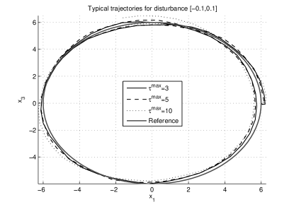
Figure 2: Closed loop trajectories in the $(x_{1},x_{3})$-plane.

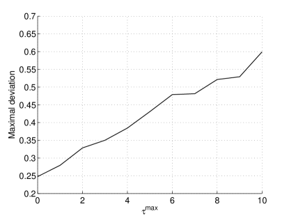
Figure 3: Maximal deviation depending on $\tau^{\max}$.

Fig. 2 shows typical trajectories and Fig. 3 the maximal deviation $\sqrt{(\|(x_{1},x_{3})^{T}\|_{2}-6)^{2}+(\|(x_{2},x_{4})^{T}\|_{2}-10)^{2}}$ depending on $\tau^{\max}$. The results confirm the robustness of the closed loop as well as the increasing sensitivity against perturbations for larger $\tau^{\max}$. Note that the deviation grows linearly in $\tau^{\max}$ since the system is open loop stable, cf. Remark 3.1.

5 Conclusions

Delays and information loss are often unavoidable in todays control systems. They must be accounted for during the controller design to avoid instability or performance decay. One way to improve the performance and to guarantee stability is the use of prediction based compensation schemes. Instead of a single input a sequence of (predicted) future controls is submitted, buffered and implemented sequentially at the actuator. The main result of this work is that so-called prediction consistent compensation and control schemes, such as, e.g., the predictive control schemes presented in Findeisen and Varutti (2009) or Grüne et al. (2009), can posses inherent robustness properties. Precisely, if the nominal closed loop system without delays is input-to-state stable (ISS), then the closed loop system subject to delays and utilizing a prediction consistent delay compensation approach is robustly stable. Additionally, we explicitly analyzed the quantitative influence of the prediction horizon and model uncertainties on the robustness gains and illustrate the results by a numerical simulation. The derived results significantly expand the applicability of prediction consistent delay compensation approaches, e.g. based on predictive control solutions, since they establish that these methods are also applicable to uncertain systems subject to disturbances.

References

- Bemporad (1998) A. Bemporad. Predictive control of teleoperated constrained systems with unbounded communication delays. In Proc. 37th IEEE Conf. on Dec. and Control, CDC’98, pages 2133–2138, 1998.
- Elaiw (2007) A. M. Elaiw. Multirate sampling and input-to-state stable receding horizon control for nonlinear systems. Nonlinear Anal., 67:1637–1648, 2007.
- Findeisen (2006) R. Findeisen. Nonlinear Model Predictive Control: a Sampled-Data Feedback Perspective. Number 1086 in Reihe 8. VDI Verlag, 2006.
- Findeisen and Allgöwer (2004) R. Findeisen and F. Allgöwer. Computational delay in nonlinear model predictive control. In Proc. Int. Symp. Adv. Contr. of Chem. Proc., pages 427–432, Hong Kong, PRC, 2004.
- Findeisen and Varutti (2009) R. Findeisen and P. Varutti. Stabilizing nonlinear predictive control over nondeterministic communication networks. In L. Magni, D. Raimondo, and F. Allgöwer, editors, Nonlinear Model Predictive Control: Towards New Challenging Applications, LNCIS 384, pages 167–179. Springer, 2009.
- Grüne and Nešić (2003) L. Grüne and D. Nešić. Optimization based stabilization of sampled-data nonlinear systems via their approximate discrete-time models. SIAM J. Control Optim., 42(1):98–122, 2003.
- Grüne et al. (2009) L. Grüne, J. Pannek, and K. Worthmann. A prediction based control scheme for networked systems with delays and packet dropouts. In Proceedings of the 48th IEEE CDC, pages 537–542, Shanghai, China, 2009.
- Hespanha et al. (2007) J.P. Hespanha, P. Naghshtabrizi, and Y. Xu. A survey of recent results in networked control systems. Proc. of the IEEE, 95(1):138–162, 2007.
- Limon et al. (2009) D. Limon, T. Alamo, D. L. Raimondo, J. M. Bravo, D. Munoy de la Pena, A. Ferramosca, and E. F. Camacho. Input-to-state stability: an unifying framework for robust model predictive control, nonlinear model predictive control. In L. Magni, D. Raimondo, and F. Allgöwer, editors, Nonlinear Model Predictive Control: Towards New Challenging Applications, LNCIS 384, pages 1–26. Springer, 2009.
- Lunze and Lehmann (2010) J. Lunze and D. Lehmann. A state-feedback approach to event-based control. Automatica, 46(1):211–215, 2010.
- Magni and Scattolini (2007) L. Magni and R. Scattolini. Robustness and robust design of MPC for nonlinear systems. In R. Findeisen, L. Biegler, and F. Allgöwer, editors, Assessment and Future Directions of Nonlinear Model Predictive Control, LNCIS 358, pages 239–254. Springer, 2007.
- Polushin et al. (2008) I. G. Polushin, P. X. Liu, and C.-H. Lung. On the model-based approach to nonlinear networked control systems. Automatica, 44:2409–2414, 2008.
- Quevedo et al. (2011) D. Quevedo, J. Østergaard, and D. Nešić. Packetized predictive control of stochastic systems over bit-rate limited channels with packet loss. IEEE Trans. Automat. Control, 2011. To appear.
- Sontag (2000) E. D. Sontag. The ISS philosophy as a unifying framework for stability–like behavior. In F. Isidori, A. Lamnabhi-Lagarrigue and W. Respondek, editors, Nonlinear Control in the Year 2000, pages 443–467. Springer, 2000.
- Varutti and Findeisen (2009) P. Varutti and R. Findeisen. Compensating network delays and information loss by predictive control methods. In Proc. of the Europ. Contr. Conf., ECC’09, pages 1722 – 1727, 2009.
- Varutti et al. (2009) P. Varutti, B. Kern, T. Faulwasser, and R. Findeisen. Event-based model predictive control for networked control systems. In Proc. of the 48th IEEE Conf. on Dec. and Cont., CDC’09, pages 567–572, 2009.
- Zavala and Biegler (2009) V.M. Zavala and L.T. Biegler. The advanced-step NMPC controller: Optimality, stability and robustness. Automatica, 45:86–93, 2009.