ARGOT: Accelerated radiative transfer on grids using oct-tree

Abstract

We present two types of numerical prescriptions that accelerate the radiative transfer calculation around point sources within a three-dimensional Cartesian grid by using the oct-tree structure for the distribution of radiation sources. In one prescription, distant radiation sources are grouped as a bright extended source when the group’s angular size, $\theta_{\rm s}$, is smaller than a critical value, $\theta_{\rm crit}$, and radiative transfer is solved on supermeshes whose angular size is similar to that of the group of sources. The supermesh structure is constructed by coarse-graining the mesh structure. With this method, the computational time scales with $N_{\rm m}\log(N_{\rm m})\log(N_{\rm s})$ where $N_{\rm m}$ and $N_{\rm s}$ are the number of meshes and that of radiation sources, respectively. While this method is very efficient, it inevitably overestimates the optical depth when a group of sources acts as an extended powerful radiation source and affects distant meshes. In the other prescription, a distant group of sources is treated as a bright point source ignoring the spatial extent of the group and the radiative transfer is solved on the meshes rather than the supermeshes. This prescription is simply a grid-based version of START by Hasegawa & Umemura and yields better results in general with slightly more computational cost ($\propto N_{\rm m}^{4/3}\log(N_{\rm s})$) than the supermesh prescription. Our methods can easily be implemented to any grid-based hydrodynamic codes and are well-suited to adaptive mesh refinement methods.

1 Introduction

Radiative transfer (RT) of photons has fundamental importance for formation of astronomical objects, such as galaxies, stars, and blackholes. Unfortunately, the nature of RT, in which we have to solve the time evolution of the six-dimensional phase-space information of photons (three spatial dimensions, two angular dimensions, and one frequency dimension; or equivalently three spatial and three momentum dimensions), makes it difficult to solve RT accurately and to couple it with hydrodynamics. To date, various RT schemes has been proposed (Iliev et al., 2006), some of which are coupled with hydrodynamics (Iliev et al., 2009). A wide range of approximation have been used to deal with multi-dimensional nature of the transfer equation and they have their own pros and cons.

When radiation sources are embedded in media on meshes, RT calculations can be categorised into two types; one premises that the source functions are assigned on meshes and the other does that radiation sources are treated as point sources independent of meshes. In the former type, the RT equations are integrated along long or short characteristics between meshes. The latter is advantageous when the number of the point sources, $N_{\rm s}$, is smaller than that of the boundary meshes, $\sim N_{\rm m}^{2/3}$, where $N_{\rm m}$ is the total number of the meshes. The latter type of the RT schemes is often called ‘ray-tracing’ that we deal with in this paper.

The most accurate and straight-forward RT scheme is the long characteristics method in which all source meshes are connected to all other relevant meshes (Abel et al., 1999; Sokasian et al., 2001; Susa, 2006). This method is however very expensive computationally. The computational costs scales with $N_{\rm m}^{2}$ in general and with $N_{\rm m}^{4/3}N_{\rm s}$ for the transfer from point sources.

The short characteristics method (Kunasz & Auer, 1988; Stone et al., 1992; Mellema et al., 1998; Nakamoto et al., 2001) reduces the computational cost by integrating the equation of RT only along lines that connect nearby cells. It scales with $N_{\rm m}^{5/3}$ and with $N_{\rm m}N_{\rm s}$ for the transfer from point sources. Its known disadvantage is the inability to track collimated radiation fields and hence the inability to cast sharp shadows owing to the numerical diffusion.

The methods whose computational cost is similar to that of the short characteristics method with small loss of accuracy compared to the long characteristics method have also been developed (Razoumov & Cardall 2005 and ‘authentic RT’ by Nakamoto et al. in Iliev et al. 2006). Adaptive ray tracing (Abel & Wandelt, 2002) has been widely used for RT around point sources (Wise & Abel, 2011).

Mote Carlo transport (Ciardi et al., 2001) is also straight forward. The advantage of this approach is that comparatively few approximations to the RT equations need to be made. The resulting radiation field however inevitably becomes noisy (see Iliev et al., 2006) due to its stochastic nature unless a huge number of photon packets are transported. This method is computationally very expensive in the optically thick regime.

The methods, which consider the moments of the RT equations and consist in choosing a closure relation to solve them, can lead to substantial simplifications that can drastically speed up the calculations because its computational cost scales with $\sim N_{\rm m}$. The most common of these methods is the flux-limited diffusion, which solves the evolution of the first moment and uses a closure relation valid in the diffusion limit, which is an isotropic radiative pressure tensor. The equation is modified with an ad-hoc function (the flux limiter) in order to ensure that the radiative flux is valid in the free-streaming limit. This method is very useful in diffusive regions and have been used to study accretion discs (Ohsuga et al., 2005) and star formation (Krumholz, 2006). Another method of closing the system is the variable Eddington tensor formalism. It gives better results than the flux-limited diffusion but are much more complex and costly because it requires the local resolution of the transfer equation at each timestep. The methods which employ the optically thin variable Eddington tensor approximation (Gnedin & Abel, 2001) have been used to study cosmic reionization (Gnedin & Abel, 2001; Ricotti et al., 2002; Petkova & Springel, 2009). A locally evaluated Eddington tensor, called the M₁ model, has also been used to close the system (González et al., 2007) and has applied to study cosmic reionization (Aubert & Teyssier, 2008). The accuracy of the moments methods is problem-dependent and is hard to judge in general situation. Petkova & Springel (2011) have developed a method that employs a direct discretisation of the RT equation in Boltzmann form with finite angular resolution on moving meshes. This method is advantageous in solving problems in which time-dependent solution of the RT equation is important. The timestep however has to be very short because photons propagate at the speed of light unless a reduced speed of light approximation is employed.

In many astrophysical problems, for example cosmic reionization and galaxy formation, we have to deal with numerous radiation sources. Pawlik & Schaye (2008) introduced source merging procedure in order to avoid computationally expensive scaling with the number of sources and implemented it on Smoothed Particle Hydrodynamics (SPH). Hasegawa & Umemura (2010) utilised the oct-tree algorithm (Barnes & Hut, 1986) in order to accelerate the RT around point sources and they coupled the RT with SPH. In their method, distant sources from a target gas particle are grouped and regarded as a single point source when the angular size of the group of the sources is smaller than a critical value. Consequently, the effective number of radiation sources is largely reduced to $\log(N_{\rm s})$ when there are $N_{\rm s}$ sources.

The methods we explore in this paper are parallel to this approach except that we implement this grouping algorithm to grid-based codes. In one of our methods, we introduce supermeshes; a supermesh consists of $8^{n}$ meshes and it is characterised by the mean density of each chemical species of the meshes within the supermesh. Solving the RT on supermeshes whose angular size is similar to that of the group of the sources in question results in further reduction of computational time in principle. Another approach we take is the point source approximation, in which a group of sources sufficiently distant from a target mesh is treated as a point source. The latter can be regarded as a grid-based version of START (Hasegawa & Umemura, 2010).

Unlike gravitational interactions to which the tree-algorithm has been widely applied, RT is affected by the medium between a source and a target. It is therefore very important to test these tree-based approaches in cases where an extended group of sources works as a powerful source in inhomogeneous medium and affects (e.g. ionizes) distant meshes. In this paper, we extensively investigate such cases in order to clarify advantages and disadvantages of the methods using tree-based algorithm.

This paper is organised as follows. In section 2, we describe the algorithm in detail. In section 3, we present several test problems and compare our methods to each other. We summarise and discuss the results in section 4.

2 Radiative transfer with tree-algorithm

In this section, we describe our ray-tracing algorithm that we use to solve the steady RT equation for a given frequency, $\nu$:

$$\frac{{\rm d}I_{\nu}}{{\rm d}\tau_{\nu}}=-I_{\nu}+S_{\nu},$$ (1)

where $I_{\nu}$, $\tau_{\nu}$, and $S_{\nu}$ are the specific intensity, the optical depth, and the source function, respectively. This equation is adequate for problems in which the absorption and emission coefficients change on timescales much longer than the light crossing time. This will always be the case in the volumes we will simulate by using our methods. Eqn. (1) has a formal solution:

$$I_{\nu}(\tau_{\nu})=I_{\nu,0}\mathrm{e}^{-\tau_{\nu}}+\int_{0}^{\tau_{\nu}}S_{\nu}(\tau^{\prime}_{\nu})\mathrm{e}^{-\tau_{\nu}+\tau^{\prime}_{\nu}}{\rm d}\tau^{\prime}_{\nu},$$ (2)

where $I_{\nu,0}$ is the specific intensity at $\tau_{\nu}=0$ and $\tau^{\prime}_{\nu}$ is the optical depth at a position along the ray. Throughout this paper we employ so-called on-the-spot approximation (Osterbrock & Ferland, 2006) in which recombination photons are assumed to be absorbed where they were emitted. Using the on-the-spot approximation, the formal solution given by equation (2) is reduced to

$$I_{\nu}(\tau_{\nu})=I_{\nu,0}\mathrm{e}^{-\tau_{\nu}}.$$ (3)

To solve this equation numerically, one needs to calculate optical depth between each pair of a source and a target mesh. The computational cost is hence proportional to the number of sources. In the next subsection, we will describe the method to decrease the effective number of radiation sources by using the oct-tree structure.

2.1 Source grouping algorithm

As in Hasegawa & Umemura (2010), we construct the oct-tree structure for the distribution of radiation sources. A cubic computational domain is hierarchically subdivided into 8 cubic cells until each cell contains only one radiation source or the size of a cell becomes sufficiently small compared to that of the computational domain. We call these sub-volumes ‘tree nodes’. When the side length of the cubic computational domain is $L$, the width of a level $l$ tree node is given by $w^{(l)}=L/2^{l}$. Each tree node records the centre of the luminosity of the radiation sources contained in the node,

$$\boldsymbol{r}=\frac{\sum_{m}\boldsymbol{r}_{m}L_{m}}{\sum_{m}L_{m}},$$ (4)

and the total luminosity,

$$L=\sum_{m}L_{m},$$ (5)

where $\boldsymbol{r}_{m}$ and $L_{m}$ indicate the position vector and the luminosity of a radiation source, respectively, and subscript $m$ runs over all sources within the tree node.

Once we have constructed the tree structure, we loop over all meshes. RT from all the radiation sources to each target mesh is performed by a simple recursive calculation as done in $N$-body calculation. We start at the root node (level 0 tree node), which covers entire computational domain. Let $w$ be the width of the node currently being processed and $D$ the distance between the closest edges of the tree node and the target mesh. If the angular size of the node is smaller than a fixed value of accuracy parameter, i.e.

$$\frac{w}{D}<\theta_{\rm crit},$$ (6)

then we perform the RT calculation between the group of sources in the current node and the target mesh and move on to the next node. Otherwise, we examine the child nodes (subnodes) recursively. The effective number of sources is thus proportional to $\log(N_{\rm s})$. In the following subsections we will explain how we perform the RT calculation between a group of sources and a target mesh.

2.2 Supermesh approximation

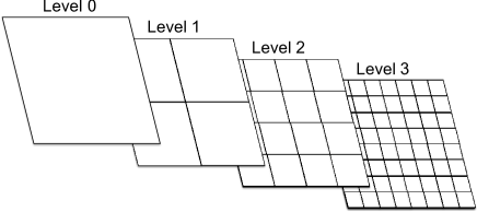
Figure 1: Schematic illustration of the supermesh structure for $8\times 8$ two-dimensional meshes. In this case, the maximum level, $l_{\rm max}$, is 3 and the meshes themselves can be used as the highest level supermeshes. A level $l$ supermesh contains $2^{2(l_{\rm max}-l)}$ meshes. For three-dimensional meshes, a level $l$ supermesh consists of $2^{3(l_{\rm max}-l)}$ meshes.

We first introduce the supermesh approximation. In Fig. 1, we show a schematic illustration of the supermesh structure. If a three-dimensional computational domain is discretised by $2^{3l_{\rm max}}$ meshes, a level $l$ supermesh consists of $2^{3(l_{\rm max}-l)}$ meshes. We can calculate the mean density of each chemical species for every supermesh by using the meshes contained in it. The meshes can be used as the highest level supermeshes. The supermesh structure is resembling to an adaptive mesh refinement (AMR) structure and thus this method is well-suited to couple with the hydrodynamics by AMR codes.

Let us consider the case in which plane-parallel radiation with the specific intensity $I_{0}$ enters a supermesh that consists of $N_{x}\times N_{y}$ meshes. What we want to know is the mean intensity of the ray emerging from the other side of the supermesh, $\langle I_{\rm out}\rangle$ (see Fig. 2).

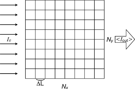
Figure 2: Plane-parallel radiation with specific intensity $I_{0}$ entering to a supermesh that consists of $N_{x}\times N_{y}$ meshes. The $(i,j)$-th mesh has the H i number density, $n_{i,j}$.

For simplicity, we here only consider the absorption by H i atoms and drop the frequency dependence. The side length of each mesh is $\Delta L$ and the H i number density of the $(i,j)$-th mesh in the supermesh is $n_{i,j}$. The mean intensity of the emerging radiation is given by

$$\langle I_{\rm out}\rangle=\frac{I_{0}}{N_{y}}\sum_{j}^{N_{y}}\exp[-\sigma_{\rm HI}{\cal N}_{j}],$$ (7)

where $\sigma_{\rm HI}$ is the H i cross-section and ${\cal N}_{j}$ is the H i column density of the $j$-th line, i.e. ${\cal N}_{j}=\sum_{i}^{N_{x}}n_{i,j}\Delta L$.

In our supermesh approximation, we use the mean H i number density, $\langle n\rangle=\sum_{i,j}n_{i,j}/(N_{x}N_{y})$, to estimate the mean intensity of the emerging radiation $\langle I_{\rm out}\rangle$. Doing this introduces some error as we will show below. In order to understand the accuracy and the nature of the supermesh approximation, we compare the mean intensity of the emerging radiation by the supermesh approximation to that calculated by using the meshes. We first consider the Taylor series expansion of the mean intensity of the emerging radiation when we solve the RT on the supermesh:

$$\langle I_{\rm out}\rangle_{\rm mean} = I_{0}\exp(-\sigma_{\rm HI}\langle{\cal N}\rangle)$$ (8)

$$= I_{0}\left[1-\sigma_{\rm HI}\langle{\cal N}\rangle+\frac{\sigma_{\rm HI}^{2}}{2}\langle{\cal N}\rangle^{2}+\cdots\right],$$

where $\langle{\cal N}\rangle$ is the mean H i column density given by

$$\langle{\cal N}\rangle=\frac{\sum^{N_{y}}_{j}{\cal N}_{j}}{N_{y}}=\frac{\Delta L\sum_{j}^{N_{y}}\sum_{i}^{N_{x}}n_{i,j}}{N_{y}}=\Delta LN_{x}\langle n\rangle.$$ (9)

On the other hand, the Taylor series expansion of Eqn. (7) is

$$\langle I_{\rm out}\rangle = \frac{I_{0}}{N_{y}}\sum_{j}^{N_{y}}\left[1-\sigma_{\rm HI}{\cal N}_{j}+\frac{1}{2}(\sigma_{\rm HI}{\cal N}_{j})^{2}+\cdots\right]$$ (10)

$$= \frac{I_{0}}{N_{y}}\left[N_{y}-\sigma_{\rm HI}\sum^{N_{y}}_{j}{\cal N}_{j}+\frac{\sigma_{\rm HI}^{2}}{2}\sum^{N_{y}}_{j}{\cal N}_{j}^{2}+\cdots\right]$$

$$= I_{0}\left[1-\sigma_{\rm HI}\langle{\cal N}\rangle+\frac{\sigma_{\rm HI}^{2}}{2}\langle{\cal N}^{2}\rangle+\cdots\right].$$

The difference between $\langle I_{\rm out}\rangle$ and $\langle I_{\rm out}\rangle_{\rm mean}$ is the second order in $\tau$. From Eqn. (7) and (8), the leading error in $\langle I_{\rm out}\rangle_{\rm mean}$ is

$$\langle I_{\rm out}\rangle-\langle I_{\rm out}\rangle_{\rm mean} = I_{0}\frac{\sigma_{\rm HI}^{2}}{2}\left(\langle{\cal N}^{2}\rangle-\langle{\cal N}\rangle^{2}\right).$$ (11)

Since the variance of the column density, $\langle{\cal N}^{2}\rangle-\langle{\cal N}\rangle^{2}$, could be very large in the inhomogeneous medium, we substantially overestimate the optical depth if we use Eqn. (8).

We can therefore in principle improve the approximation by estimating the variance of the column density. According to the central limit theorem, the variance of the column density for large $N_{x}$ can be expressed by using the variance of the density, if the density, $n_{i,j}$, is a sequence of independent and identically distributed random variables:

$$\langle{\cal N}^{2}\rangle-\langle{\cal N}\rangle^{2}=N_{x}\left[\langle n^{2}\rangle-\langle n\rangle^{2}\right].$$ (12)

Using this relation, the mean intensity of the emerging radiation can be approximated as:

$$\langle I_{\rm out}\rangle_{\rm variance} = I_{0}\biggl{[}\exp\left(-\sigma_{\rm HI}\langle{\cal N}\rangle\right)$$ (13)

$$\hskip 28.45274pt+\frac{\sigma_{\rm HI}^{2}N_{x}}{2}\left(\langle n^{2}\rangle-\langle n\rangle^{2}\right)\biggl{]}.$$

The effective column density for a ray segment that intersects the supermesh is hence

$${\cal N}_{\rm eff}=-\frac{\ln\left[\exp\left(-\sigma_{\rm HI}\langle n\rangle h\right)+\frac{\sigma_{\rm HI}^{2}h}{\Delta L}\left(\langle n^{2}\rangle-\langle n\rangle^{2}\right)\right]}{\sigma_{\rm HI}},$$ (14)

where $h$ is the length of a ray segment. We however do not employ this approximation because Eqn. (12) is only valid for large $N_{x}$ and $N_{x}$ always becomes small near the target mesh. We thus only use the mean density in our supermesh approximation which is described by Eqn. (8). We will investigate the accuracy of this approximation in Section 3.

Now we have to determine on which supermeshes we perform the RT calculation. We chose to use the lowest level supermeshes whose angular size, $\theta$, is equal to or smaller than the angular size of a group of the sources, $\theta_{\rm s}$, since we assume plane-parallel radiation to construct the approximation. We define the luminosity-weighted rms projected radius as the effective projected size of the group of the sources, i.e. if the target mesh is located along the $z$-direction from the centre of the luminosity, the projected size of the group is defined as

$$r_{\rm rms}^{2}=\frac{\sum_{m}L_{m}\left\{(x_{m}-\bar{x})^{2}+(y_{m}-\bar{y})^{2}\right\}}{\sum_{m}L_{m}},$$ (15)

where $\bar{x}$ and $\bar{y}$ are, respectively, the $x$ and $y$ components of the position vector of the luminosity centre and the subscript $m$ runs over all sources in the tree node in question. Practically, we calculate the following tensor for each tree node:

$${\cal I}_{ij}=\sum_{m}L_{m}(\boldsymbol{r}_{m,i}-\bar{\boldsymbol{r}}_{i})(\boldsymbol{r}_{m,j}-\bar{\boldsymbol{r}}_{j}),$$ (16)

where the subscripts $i$ and $j$, respectively, indicate $i$-th and $j$-th components of the position vector, i.e. $i$ and $j$ are either $x$, $y$, or $z$; and the subscript $m$ has the same meaning as in Eqn. (15). By using $(0,0)$ and $(1,1)$ components of the tensor ${\cal I}^{\prime}$ which is the tensor ${\cal I}$ in the rotated frame so that the target mesh is placed along the $z$-direction from the luminosity centre, we can estimate the angular size of the group of the source in the tree node as

$$\theta_{\rm s}=\frac{2r_{\rm rms}}{D}=\frac{2}{D}\left(\frac{{\cal I}^{\prime}_{00}+{\cal I}^{\prime}_{11}}{\sum_{m}L_{m}}\right)^{\frac{1}{2}},$$ (17)

where $D$ is the distance between the luminosity centre and the closest edge of the target mesh. In Fig. 3, we illustrate the procedure of the RT calculation using the supermeshes.

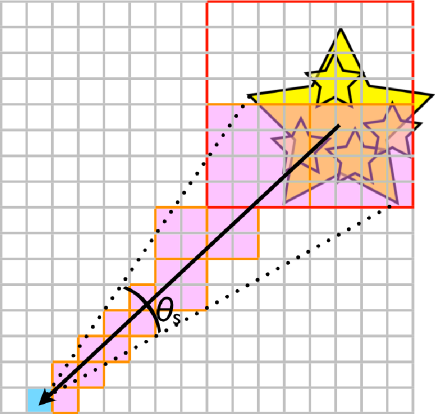
Figure 3: A schematic illustration of the RT calculation using supermeshes. The radiation sources in the tree node indicated by red square are regarded as a single bright extended source. The target mesh is coloured by light blue. The RT is solved on the supermeshes at the lowest level, whose angular size is equal to or smaller than the angular size of the source group, $\theta_{\rm s}$. The supermeshes used are indicated by purple colour and their sizes are represented by the orange squares.

The computational cost by this method is expected to scale with $N_{\rm m}\log(N_{\rm m})\log(N_{\rm s})$.

2.3 Point source approximation

Here we introduce another way of accelerating the RT calculation by using the oct-tree structure of the distribution of radiation sources. As in Hasegawa & Umemura (2010), we treat a group of sources in a tree node which satisfies the condition described by Eqn. (6) as a bright point source. Since we ignore the size of the source group, we solve the RT not on the supermeshes but on the meshes. Consequently, the computational cost scales with $N_{\rm m}^{\frac{4}{3}}\log(N_{\rm s})$. Although this is slightly more expensive computationally than the supermesh approximation in which the cost is proportional to $N_{\rm m}\log(N_{\rm m})\log(N_{\rm s})$, this method may faster than the supermesh approximation for small $N_{\rm m}$ because we do not have to calculate ${\cal I}^{\prime}_{00}$ and ${\cal I}^{\prime}_{11}$ in the point source approximation. Since the surface area of a Strömgren sphere is proportional to $\dot{N}^{2/3}$ where $\dot{N}$ is photoionization rate (see Section 3.1), treating a source group as a point source underestimates the surface area of ionized regions. We will explore this effect in our tests.

Table 1: Rates adopted by the code. The lines are, from top to bottom, reference for: Case B recombination rates (RRB) of H ii, He ii, and He iii ; dielectronic recombination rate (DRR) of He ii; collisional ionization rates (CIR) of H i, He i, and He ii; Case B recombination cooling rates (RCRB) of H ii, He ii, and He iii; dielectronic recombination cooling rate (DRCR) of He ii; collisional ionization cooling rates (CICR) of H i, He i, and He ii; collisional excitation cooling rates (CECR) of H i, He i, and He ii; bremsstrahlung cooling rate (BCR); inverse Compton cooling rate (CCR); photoionization cross-sections (CS) of H i, He i, and He ii.

RRB	DRR	CIR	RCRB	DRCR	CICR	CECR	BCR	CCR	CS
(4), (5), (4)	(2)	(7), (7), (1)	(4), (5), (4)	(3)	(3), (3), (3)	(3), (3), (3)	(4)	(6)	(8)

(1) Abel et al. (1997); (2) Aldrovandi & Pequignot (1973); (3) Cen (1992); (4) Hummer (1994); (5) Hummer & Storey (1998); (6) Ikeuchi & Ostriker (1986); (7) Janev et al. (1987); (8) Osterbrock & Ferland (2006)

2.4 Non-equilibrium chemistry

We solve the non-equilibrium chemistry for e, H i, H ii, He i, He ii, and He iii implicitly. Note that since we employ the on-the-spot approximation, we use ‘Case B’ recombination coefficients to calculate recombination rates of H ii, He ii, and He iii throughout this paper.

Using the optical depth obtained by the methods described in Section 2.2 or 2.3, the photoionization rates of H i, He i, and He ii in each mesh are given by

$$\Gamma_{i}=\sum_{\alpha}\Gamma_{i,\alpha},$$ (18)

where $\Gamma_{i,\alpha}$ denotes the radiative contribution from a radiation source (or a group of radiation sources), $\alpha$, and $i=\mbox{\text{H\,{i}}}$, He i, and He ii. The contribution from a point-like radiation source, $\alpha$, is represented by

$$\Gamma_{i,\alpha}=\frac{1}{4\pi hr_{\alpha}^{2}}\int_{\nu_{i}}^{\infty}\frac{{\rm d}\nu}{\nu}\sigma_{i}(\nu)L_{\alpha}(\nu)\exp\left[-\sum_{j}{\cal N}_{j,\alpha}\sigma_{j}(\nu)\right],$$ (19)

where $\nu_{i}$ is the threshold frequency for the $i$-th species, $\sigma_{i}(\nu)$ is the cross-section of the $i$-th species, and $r_{\alpha}$, $L_{\alpha}(\nu)$, and ${\cal N}_{i,\alpha}$ are respectively the distance between the luminosity centre and the target mesh, the intrinsic luminosity of the radiation source (or the group of the sources), and the column density of $i$-th species. The sum in the exponent runs over all three chemical species. When all sources have the same spectral shape, i.e. $L_{\alpha}(\nu)=C_{\alpha}f(\nu)$, we generate a look-up table for each species as a function of column densities:

$$g_{i}({\cal N}_{k})=\int_{\nu_{i}}^{\infty}\frac{{\rm d}\nu}{\nu}\sigma_{i}(\nu)f(\nu)\exp\left[-\sum_{j}{\cal N}_{j}\sigma_{j}(\nu)\right].$$ (20)

In our case, a look-up table for each chemical species becomes three-dimensional table. We have confirmed that 20 logarithmic bins for each column density is sufficient. By using the look-up tables, the RT calculation is reduced to evaluating the column densities.

Following Anninos et al. (1997), we update the densities of each chemical species implicitly by using a backward difference formula (BDF). The equations to evolve the density of each species can be generally written as

$$\frac{{\rm d}n_{i}}{{\rm d}t}=C_{i}(T,n_{j})-D_{i}(T,n_{j})n_{i},$$ (21)

where $n_{i}=\rho_{i}/(A_{i}m_{\rm H})$, $A_{i}$ is the atomic mass number of the $i$-th species, and $m_{\rm H}$ is the proton mass. This time $i$ is either e, H i, H ii, He i, He ii or He iii. The first term of the right-hand side, $C_{i}$, is the collective source term responsible for the creation of the $i$-th species. The second term involving $D_{i}$ represents the destruction mechanisms for the $i$-th species and are thus proportional to $n_{i}$.

Since the timescales for the ionization and recombination differ by many orders of magnitude depending on chemical species, Eqn. (21) is a stiff set of differential equations. In numerically solving a stiff set of equations, implicit schemes are required unless an unreasonably small timestep is employed. As in Anninos et al. (1997) we adopt a BDF. Discretisation of Eqn. (21) yields

$$n_{i}^{t+\Delta t}=\frac{C_{i}^{t+\Delta t}\Delta t+n_{i}^{t}}{1+D_{i}^{t+\Delta t}\Delta t},$$ (22)

where all source terms are evaluated at the advanced timestep. However, not all source terms can be evaluated at the advanced timestep due to the intrinsic nonlinearity of Eqn. (21). We hence sequentially update densities of all species in the order of increasing ionization states rather than updating them simultaneously; We evaluate the source terms contributed by the ionization from and recombination to the lower states at the advanced timesteps. This method has been found to be very efficient and accurate (e.g. Anninos et al., 1997; Yoshikawa & Sasaki, 2006).

Further improvements in accuracy and stability can be made by subcycling the rate solver over a single timestep with which the RT is solved. The subcycle timestep, which we call the ‘chemical timestep’, is determined so that the maximum fractional change in the electron density is limited to 10% per timestep:

$$\Delta t_{\rm chem}=0.1\left|\frac{n_{\rm e}}{\dot{n}_{\rm e}}\right|.$$ (23)

2.5 Photo-heating and radiative cooling

Similarly to the photoionization, photo-heating rate for each mesh due to the photoionization of the $i$-th species is given by

$${\cal H}_{i}=\sum_{\alpha}{\cal H}_{i,\alpha},$$ (24)

where ${\cal H}_{i,\alpha}$ indicates the contribution from a radiation source (or a group of sources), $\alpha$, and $i=\mbox{\text{H\,{i}}}$, He i, and He ii. The total photo-heating rate is defined by ${\cal H}=\sum_{i}{\cal H}_{i}n_{i}$. The contribution from a point-like source, $\alpha$, is written as

$${\cal H}_{i,\alpha}=\frac{1}{4\pi r_{\alpha}^{2}}\int_{\nu_{i}}^{\infty}\frac{{\rm d}\nu}{\nu}\sigma_{i}(\nu)L_{\alpha}(\nu)(\nu-\nu_{i})\exp\left[-\sum_{j}\sigma_{j}(\nu){\cal N}_{j,\alpha}\right].$$ (25)

As for the photoionization, we generate a look-up table for each species when all sources have the identical spectral shape.

We solve the energy equation for each mesh implicitly as

$$u^{t+\Delta t}=u^{t}+\frac{{\cal H}^{t+\Delta t}-\Lambda(n_{i}^{t+\Delta t},T^{t+\Delta t})}{\rho^{t}}\Delta t,$$ (26)

where $u$ and $T^{t}=T(n_{i}^{t},u^{t})$ are respectively the specific internal energy and temperature of the gas and $\Lambda$ is the cooling function. Although this implicit integration is always stable, we need to subcycle the energy solver with $\Delta t_{\rm chem}$ because both $C_{i}$ and $D_{i}$ in Eqn. (22) are functions of the temperature. We thus perform the rate solver and the energy solver alternately. The chemical timestep $\Delta t_{\rm chem}$ is recalculated before every subcycle.

2.6 Chemical reaction and cooling rates

We try to use the chemical reaction and cooling rates as up-to-date as possible. The sources of these rates are summarised in Table 1. Note that there are notable differences in the recombination cooling rates between literatures (see Iliev et al., 2006).

2.7 Time stepping

Since the optical depth $\tau(\nu)$ at $t+\Delta t$ depends on densities of all species at $t+\Delta t$, we have to solve the static RT equation (Eqn. (3)), the chemical reactions (Eqn. (22)), and the energy equation (Eqn. (26)) iteratively. We iterate these steps until the relative difference in the electron number density becomes sufficiently small: $|n_{\rm e}^{(n)}-n_{\rm e}^{(n-1)}|/n_{\rm e}^{(n)}<\epsilon$, where superscripts indicate the number of iterations and we set $\epsilon$ to $10^{-4}$ throughout this paper. The timestep $\Delta t$, with which we solve the RT equation to obtain $\Gamma_{i}^{t+\Delta t}$ and ${\cal H}_{i}^{t+\Delta t}$, could be much larger than the chemical timestep $\Delta t_{\rm chem}$, with which we subcycle the rate and energy solvers.

We however choose to employ a timestep that is defined by the timescale of the chemical reactions:

$$\Delta t_{i}=\epsilon_{\rm e}\left|\frac{n_{\rm e}}{\dot{n}_{\rm e}}\right|_{i}+\epsilon_{\rm HI}\left|\frac{n_{\rm HI}}{\dot{n}_{\rm HI}}\right|_{i},$$ (27)

where the second term in the right-hand side prevent the timestep from becoming too short when the medium is almost neutral. Our choice for $\epsilon_{\rm e}$ and $\epsilon_{\rm HI}$ are 0.2 and 0.002, respectively. We follow the evolution of the system with the minimum of the timestep defined by Eqn. (27), i.e.

$$\Delta t=\Delta t_{i,{\rm min}}.$$ (28)

The timestep $\Delta t$ is therefore only about twice as long as the shortest chemical timestep, $\Delta t_{{\rm chem},{\rm min}}$. With this timestep, we find the solutions typically within 3 to 6 iteration steps. While we can of course use a longer timestep, a longer timestep requires more iterations and the total number of steps becomes similar or even larger than the case we employ the timestep defined by Eqn. (28). With a longer timestep, the solutions sometimes never converge. This timestep is in general much shorter than the timestep defined by the Courant timestep criterion and therefore we have to subcycle the hydrodynamical timestep with this timestep when we couple the RT with the hydrodynamics.

When optically thick meshes exist, the solutions converge very slowly. We thus use smoothed photoionization rates, $\tilde{\Gamma}_{i}$, and heating rates, $\tilde{\cal H}_{i}$, instead of $\Gamma_{i}$ and ${\cal H}_{i}$. The smoothed rates for the $i$-th mesh is calculated by using adjacent 26 meshes, i.e. 27 meshes in total, with a Gaussian kernel of the smoothing length $\Delta L$. Doing this drastically reduces the number of iterations required to find the solutions. This smoothing may introduce the smearing of the I-fronts especially when the spacial resolution is poor. While we do not find such an effect in our test simulations as we will show later, this can be avoided by applying the smoothing only to optically thick meshes as done by Susa (2006).

3 Test simulations

In this section, we describe the tests we perform. In order to evaluate the accuracy of our tree-based RT algorithms, problems should involve many sources. Therefore some of the tests presented are neither simplest nor cleanest. All test problems are solved in three dimensions, with $128^{3}$ meshes unless otherwise stated.

3.1 Test 1 – Pure hydrogen isothermal H ii region expansion

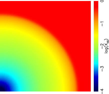
Figure 4: Test 1 – Images of the H i fraction, cut through at the mid plane of the simulation box at $t=500~{}{\rm Myr}$.

The first test is the classical problem of a H ii region expansion in a static, homogeneous, and isothermal gas, which consists of only hydrogen, around a single ionizing source. This problem has a known analytic solution and is therefore the most widely used test. Note however that since there is only a single radiation source, our RT schemes described in Sections 2.2 and 2.3 have no difference and both methods become the long characteristics method. The aim of this test is hence to test our chemical reaction solver and time stepping procedure.

We adopt a monochromatic radiation source that steadily emits $\dot{N}_{\gamma}$ photons per second, whose frequency is the Lyman limit frequency ($h\nu_{\rm L}=13.6$ eV). The density of the initially neutral gas is $n_{\rm H}$. Assuming the ionization equilibrium, the Strömgren radius is given by

$$r_{\rm S}=\left(\frac{3\dot{N}_{\gamma}}{4\pi\alpha_{\rm B}(T)n_{\rm H}^{2}}\right)^{1/3},$$ (29)

where $\alpha_{\rm B}$ is the Case B recombination coefficient. If we assume that the ionization front (I-front) is infinitely thin, the evolution of the I-front radius is analytically given by

$$r_{\rm I}=r_{\rm S}\left[1-\exp(-t/t_{\rm rec})\right]^{1/3},$$ (30)

where

$$t_{\rm rec}=\left(n_{\rm H}\alpha_{\rm B}\right)^{-1}$$ (31)

is the recombination time.

The analytical solution for the profile of the neutral and ionized fractions ($X_{\rm HI}(r)=n_{\rm HI}(r)/n_{\rm H}$ and $X_{\rm HII}(r)=n_{\rm HII}(r)/n_{\rm H}$) can also be calculated (e.g. Osterbrock & Ferland, 2006) from the equation of the ionization balance at radius $r$:

$$\frac{n_{\rm HI}(r)}{4\pi r^{2}}\dot{N}_{\gamma}e^{-\tau(r)}\sigma_{\rm HI}(\nu_{\rm L})=n_{\rm HII}(r)^{2}\alpha_{\rm B}(T),$$ (32)

where

$$\tau(r)=\sigma_{\rm HI}\int_{0}^{r}n_{\rm HI}(r^{\prime}){\rm d}r^{\prime}.$$ (33)

The profile of the neutral fraction is thus given by

$$X_{\rm HI}(r)=\frac{2+\frac{\dot{N}_{\gamma}e^{-\tau(r)}\sigma_{\rm HI}}{4\pi r^{2}n_{\rm H}\alpha_{\rm B}}-\sqrt{\left(2+\frac{\dot{N}_{\gamma}e^{-\tau(r)}\sigma_{\rm HI}}{4\pi r^{2}n_{\rm H}\alpha_{\rm B}}\right)^{2}-4}}{2}.$$ (34)

To derive this profile, we ignore the collisional ionization, which is included in our simulations.

The initial physical parameters of this test are the same as those of Test 1 in Cosmological Radiative Transfer Comparison Project (Iliev et al., 2006), where the hydrogen number density, $n_{\rm H}$, is $10^{-3}~{}{\rm cm}^{-3}$, the temperature of the isothermal gas is $10^{4}$ K, and ionization rate, $\dot{N}_{\gamma}$, is $5\times 10^{48}$ photons s^-1. Given these parameters and the recombination rate we use, $\alpha_{\rm B}(10^{4}~{}{\rm K})=2.58\times 10^{-13}~{}{\rm cm}^{3}~{}{\rm s}^{-1}$, the recombination time and the Ströemgren radius are $t_{\rm rec}=122.6~{}{\rm Myr}$ and $r_{\rm S}=5.4~{}{\rm kpc}$, respectively.

We employ identical numerical parameters to those in Iliev et al. (2006): The side length of the simulation box is 6.6 kpc, initial ionization fraction is set to $1.2\times 10^{-3}$, and a radiation source is placed at the corner of the box, $(0,0,0)$. We compare our simulation results to the analytical solution given by Eqn. (34) which represents the solution at $t=\infty$.

In Fig. 4, we show the neutral fraction in the $z=0.5\Delta L$ plane at $t=500~{}{\rm Myr}$, at which point the I-front is close to to the maximum radius, i.e. the Strömgren radius. The H ii region is nicely spherical, though this is not surprising because, with a single source, our method is identical to the long characteristics method.

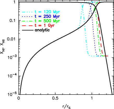
Figure 5: Test 1 – The profiles of ionized and neutral fractions. The radius is in units of the Strömgren radius. The dot-dot-dot-dashed, dotted, dot-dashed, and dashed lines represent simulated results at $t=120$, 250, 500, and 1000 Myr, respectively. The solid line indicates the analytical solution at $t=\infty$ given by Eqn. (34). The minimum ionized fraction in the numerical results is set by the collisional ionization which is not included in the analytical solution.

In Fig. 5, we show the profiles of ionized and neutral fractions at $t=120$, 250, 500, and 1000 Myr. The results asymptotically approach to the analytical solution at $t=\infty$. There is a minimum neutral fraction in the simulation results, which is set by the collisional ionization that is not included in the analytical solution.

3.2 Test 2 – Pure hydrogen H ii region expansion with thermal evolution

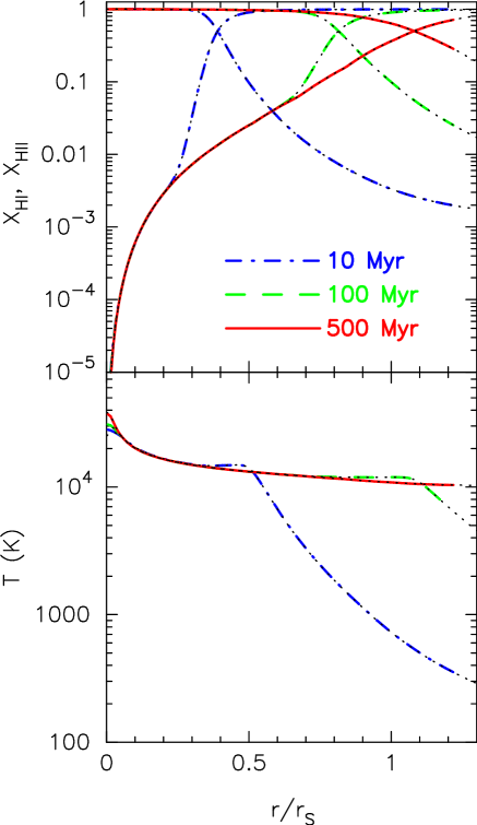
Figure 6: Test 2 – Upper panel: Spherically averaged ionized and neutral fraction profiles. The dot-dashed, dashed, and solid lines indicate indicate the profile at $t=10$, 100, and 500 Myr, respectively. The results from a high-resolution spherically symmetric one-dimensional simulation are shown by the dotted lines, which almost perfectly overlap with those by the three-dimensional simulation. The radius is in units of the Strömgren radius for the uniform isothermal gas with $n_{\rm H}=10^{-3}~{}{\rm cm}^{-1}$ and $T=10^{4}$ K. Lower panel: Spherically averaged temperature profiles. The meaning of the lines is the same as in the upper panel.

Test 2 solves essentially the same problem as Test 1, but the ionizing source is assumed to have a $10^{5}$ K blackbody spectrum and we allow the gas temperature to vary owing to heating and cooling processes. The initial gas temperature and ionized fraction are set to $10^{2}$ K and $1.2\times 10^{-3}$, respectively.

In Fig. 6, we show the neutral and ionized fraction profiles (upper panel) and the temperature profiles (lower panel) at $t=10$, 100, and 500 Myr. We also show the results from a high-resolution spherically symmetric one-dimensional simulation by the dotted line. For the one-dimensional simulation, we use 1024 meshes for a sphere of radius of $1.5\times r_{\rm S}$ and we do not employ the smoothed ionization and heating rates whereas smoothed rates are employed in the tree-dimensional simulation. The results by the three-dimensional simulation are almost indistinguishable from those obtained by the one-dimensional one. The use of the smoothed rates to accelerate the convergence has thus no evident side-effects such as smearing of the I-front.

For this test, our results are most resembling to those obtained by RSPH for Test 2 in Cosmological Radiative Transfer Comparison Project (Iliev et al., 2006). The agreement with RSPH is natural because both methods are essentially the long characteristics method. Small differences are probably caused by different adopted rates.

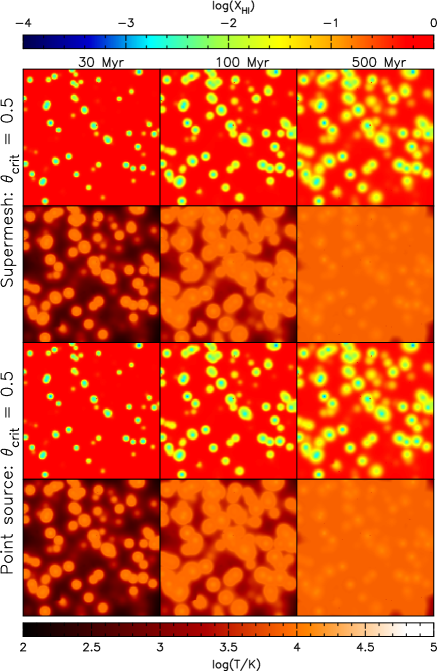
Figure 7: Test 3 – Images of the H i fraction and temperature, cut through at the mid plane of the simulation box at $t=30$, 100, and 500 Myr from left to right. The side length of the simulation box is 132 kpc in which we randomly distribute 1000 radiation sources and 1000 optically thick meshes. Upper two rows show results by the supermesh approximation with $\theta_{\rm crit}=0.5$ and lower two rows by the point source approximation with $\theta_{\rm crit}=0.5$.

3.3 Test 3 – Multiple radiation sources in a clumpy medium

In order to test the validity of the RT solver based-on the source grouping, we have to solve problems that involve multiple sources. Moreover, the error in the supermesh approximation becomes large when the inhomogeneity of the medium is large (see Eqn. (11)). In this test, we therefore solve the RT from multiple sources in the clumpy medium. The side length of the simulation box is 132 kpc. We randomly select 1000 optically thick meshes whose hydrogen number density is $n_{\rm H}=0.2~{}{\rm cm}^{-3}$ and optical depth at the Lyman limit frequency is $\sim 4\times 10^{3}$ for the mesh size. The hydrogen number density of other meshes is set to $n_{\rm H}=10^{-3}~{}{\rm cm}^{-3}$. We also randomly distribute 1000 radiation sources in the simulation box. Each source has a $10^{5}$ K blackbody spectrum and steadily emits $\dot{N}_{\gamma}=5\times 10^{48}$ ionizing photons per second. The initial gas temperature and ionization fraction are set to $10^{2}$ K and $1.2\times 10^{-3}$, respectively.

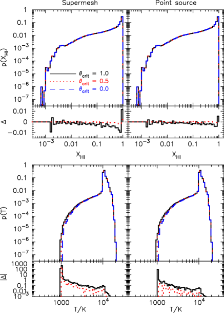
Figure 8: Test 3 – Dependence on the accuracy parameter $\theta_{\rm crit}$. Upper panels: The volume fractions of the neutral fraction at $t=500$ Myr. The results by the supermesh approximation are presented in the left panel. The solid (black), dotted (red), and dashed (blue) lines indicate the results with $\theta_{\rm crit}=1.0$, $0.5$, and $0.0$, respectively. The relative difference to the long characteristics method ($\theta_{\rm crit}=0$), $\Delta$, is also shown. The right panel shows the results obtained by the point source approximation. Lower panels: The volume fractions of the gas temperature at $t=500$ Myr. The meaning of the lines are the same as in the upper panels.

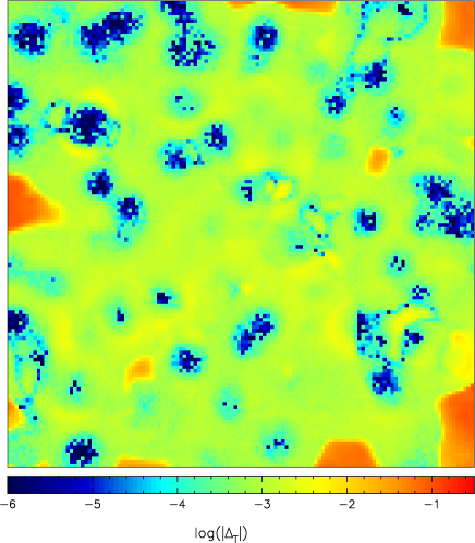
Figure 9: Test 3 – Relative difference in the temperature, cut through at the mid plane of the simulation box at $t=500~{}{\rm Myr}$. This figure compares temperature obtained by the supermesh approximation with $\theta_{\rm crit}=1$ to that by the long characteristics method ($\theta_{\rm crit}=0$). The relative difference in temperature is defined as $\Delta_{T}=(\left.T\right|_{\theta_{\rm crit}=1}^{\rm supermesh}-\left.T\right|^{\rm long})/\left.T\right|^{\rm long}$.

In Fig. 7, we show the neutral fraction and temperature maps at the mid plane of the simulation box at $t=30$, 100, and 500 Myr. We show the results by the supermesh approximation and by the point source approximation with $\theta_{\rm crit}=0.5$. The results by two methods are virtually identical to each other including the shape of shadows by the optically thick meshes.

In order to investigate the dependence on the accuracy parameter $\theta_{\rm crit}$, we compare the simulations with $\theta_{\rm crit}=1$, 0.5, and 0. In Fig. 8, we show the volume fractions of the neutral fraction and the volume fractions of the gas temperature respectively in the upper panels and lower panels. We also show difference in the volume fractions relative to those obtained by the long characteristics method ($\theta_{\rm crit}=0$). For example, the relative difference in the volume fraction of the neutral fraction by the supermesh approximation with $\theta_{\rm crit}=x$ is defined as

$$\Delta=\frac{\left.p(X_{\mbox{\text{H\,{i}}}})\right|_{\theta_{\rm crit}=x}^{\rm supermesh}-\left.p(X_{\mbox{\text{H\,{i}}}})\right.|_{\rm long}}{\left.p(X_{\mbox{\text{H\,{i}}}})\right|_{\rm long}}.$$ (35)

The volume fractions of the neutral fraction with $\theta_{\rm crit}=1$ and $0.5$ agree quite well with those by the long characteristics method ($\theta_{\rm crit}=0$). The relative differences are typically less than 1 % even with $\theta_{\rm crit}=1$. For a given value of the accuracy parameter, the point source approximation shows slightly better agreement with the long characteristics method. On the other hand, agreement in the volume fraction of the gas temperature is not as excellent as that for the neutral fraction. In particular, both the supermesh and point source approximation predict much more low temperature gas around $10^{3}$ K. This is because treating a source group as a point source underestimates the surface are of the ionized regions as we stated in Section 2.3 and the low temperature gas is primarily heated by high energy photons that permeate beyond the surfaces of highly ionized regions. Except for this disagreement for the low temperature gas ($\lesssim 2\times 10^{3}$ K), typical difference is less than 10 %.

To study how serious the deviation from the long characteristics method at low temperature, we compare the temperature map obtained by the supermesh approximation ($\theta_{\rm crit}=1$), which shows the worst agreement with the long characteristics method, and that by the long characteristics method in Fig. 9. We find that the temperature difference is largest for the low temperature gas with $T\sim 10^{3}~{}{\rm K}$ (see also Fig. 7). The difference in temperature is however very small, only 10 % at most. We therefore conclude that the results with $\theta_{\rm crit}=1$ are almost converged to the result obtained by the long characteristics method.

This test proves that both tree-based methods produce equally good results even with a large value of the accuracy parameter, $\theta_{\rm crit}=1$, in the situation where a local H ii region is driven primarily by one or a few sources. This situation is resembling to the early stage of cosmic reionization. Only at very late stage of the reionization, the H ii regions overlap each other and multiple sources become visible each other; at this stage, the reionization has largely completed already. We thus expect that our tree-based methods, in particular the supermesh approximation, are well suited to this type of problems.

3.4 Test 4 – Clustered radiation sources in a clumpy medium

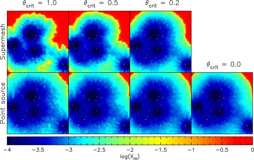
Figure 10: Test 4 – H i fraction maps, cut through the simulation box at coordinate $z=63.5\Delta L=65.5~{}{\rm kpc}$ at time $t=100$ Myr. From left to right, the values of the accuracy parameters are $\theta_{\rm crit}=1.0$, 0.5, 0.2, and 0.0 respectively. The upper panels show results by the supermesh approximation and the lower panels display those by the point source approximation.

Unlike Test 3, here we explore the problem in which groups of sources act like bright extended sources and they ionize distant meshes. This would be one of the toughest problems for the methods accelerated by source grouping. The side length of the simulation box is the same as in Test 3, i.e. $L_{\rm box}=132$ kpc. In order to construct clustered distribution of radiation sources, we put a sphere of radius $r=L_{\rm box}/4$, whose centre is randomly placed in the simulation box. We uniformly distribute 1000 radiation sources in the sphere. We then put a new sphere whose radius is 20% smaller than the previous one and again we distribute 1000 sources in the sphere. We continue this procedure until we put 10 spheres, each of which contains 1000 sources. Consequently, there are $10^{4}$ radiation sources in the simulation box. Each source has a $10^{5}$ K blackbody spectrum and emits $\dot{N}_{\gamma}=5\times 10^{48}$ ionizing photons per second. We also randomly select $10^{4}$ optically thick meshes whose hydrogen number density is $n_{\rm H}=0.2~{}{\rm cm}^{-3}$. The hydrogen number density of the remaining meshes is set to $n_{\rm H}=10^{-3}~{}{\rm cm}^{-3}$. The initial gas temperature and ionization fraction are set to $10^{2}$ K and $1.2\times 10^{-3}$, respectively.

In Fig. 10, we show the neutral fraction maps, cut through at the mid plane of the simulation box. The size and shape of the ionized regions by the supermesh approximation strongly depend on the value of the accuracy parameter; The larger the value is, the smaller the size of the ionized regions is. This is due to the very nature of the supermesh approximation, which significantly overestimates the optical depth when a size of supermesh is large and the variance of the H i density is large (see Eqn. (11) and (12)). On the other hand, the results by the point source approximation are relatively insensitive to the value of the accuracy parameter. The size of the ionized regions is almost same between $\theta_{\rm crit}=1$ and 0 while small difference is seen in the shapes.

In Fig. 11, we show the volume fractions of the neutral fraction and gas temperature at $t=100$ Myr varying the value of the accuracy parameter, $\theta_{\rm crit}$, from 1 to 0. We also show the relative difference to the long characteristics method ($\theta_{\rm crit}=0$). The volume fraction of the neutral fraction confirms the dependence of the supermesh approximation on the value of the accuracy parameter, i.e. the larger the value of $\theta_{\rm crit}$ is, the smaller the ionized fraction is. This dependence is more evident in the volume fraction of the gas temperature. There is more low temperature gas in the simulation with a larger value of the accuracy parameter. Importantly, the results by the supermesh approximation with $\theta_{\rm crit}=0.2$ still significantly deviate from those by the long characteristics methods, and therefore we cannot trust the result even with $\theta_{\rm crit}=0.2$.

On the other hand, the result by the point source approximation with $\theta_{\rm crit}=1$ shows an excellent agreement with that with the long characteristics method, in spite of the fact that this approximation ignores the spatial extent of source groups. This result proves that the point source approximation is very efficient and accurate for this type of problems.

The relative difference to the long characteristics method indicates that both approximations overestimates the volume fraction of the almost fully-ionized gas ($X_{\mbox{\text{H\,{i}}}}\simeq 2\times 10^{-6}$). This ionized fraction corresponds to the central regions of each source spheres. The volume of these regions are however very small and the neutral fraction is very low anyway; this overestimation of the ionization fraction at the central regions of the source spheres does not affect the evolution of the whole simulation box. In fact, by the point source approximation, the relative difference to the long characteristics method in the volume fraction of the neutral fraction is typically 1 % and $\sim 10$ % at most except for the highly ionized gas with $X_{\mbox{\text{H\,{i}}}}\lesssim 10^{-5}$.

Even by the point source approximation, the relative difference in the volume fraction of the gas temperature to the long characteristics method is rather large for the low temperature gas. The gas temperature however agrees very well with that by the long characteristics method just as we showed for Test 3. Except for the low temperature gas, the typical difference is $\sim 10$ %. Interestingly, decreasing the value of the accuracy parameter in the point source approximation from 1 to 0.2 does not improve the agreement with the long characteristics method very much in spite of the fact that the simulations with a smaller value of the accuracy parameter is much more computationally expensive as we will show in the next subsection. Since the point source approximation with $\theta_{\rm crit}=1$ seems to be sufficiently accurate, we expect that this approximation with $\theta_{\rm crit}=0.5$ would be a safe choice for most types of problems.

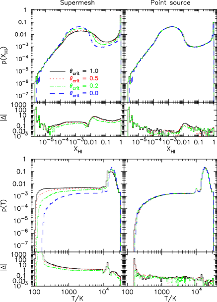
Figure 11: Test 4 – Dependence on the accuracy parameter $\theta_{\rm crit}$. Results at $t=100$ Myr are presented. The results are displayed in the same manner as Fig. 8. The volume fractions for the simulation with $\theta_{\rm crit}=1$, 0.5, 0.2, and 0 are indicated by the solid (black), dotted (red), dot-dashed (green), and dashed (blue) lines, respectively.

3.5 Code performance

We here investigate how the computation time scales with the number of meshes and that of the sources. For this purpose, we measure the wall-clock time taken for one step of the RT calculation. The computation time for solving chemistry etc. is not included. We use 8 cores of 2.13 GHz Xeon E5506 processors for these simulations.

In order to study the scaling with the number of the meshes, we randomly place 1000 radiation sources in the simulation box. Each source and the simulation box is the same as used in Test 1 except that there are 1000 sources and we vary the number of the meshes. We show the result in the upper panel of Fig. 12. We find that the supermesh approximation is slightly faster than the point source approximation for a given set of $N_{\rm m}$ and $\theta_{\rm crit}$. The computation time by the point source approximation is a slightly steeper function of the number of the meshes than that by the supermesh approximation. The computation time by the point source approximation scales with $N_{\rm m}^{4/3}$ as expected. The scaling of the computation time by the supermesh approximation is somewhere between $\propto N_{\rm m}\log(N_{\rm m})$ and $\propto N_{\rm m}^{4/3}$. Since the RT is solved on the supermeshes whose angular size is similar to the angular size of the source group, $\theta_{\rm s}$, which can be much smaller than $\theta_{\rm crit}$, the computation time becomes steeper function of $N_{\rm m}$ than the expected scaling, $\propto N_{\rm m}\log(N_{\rm m})$.

In the lower panel of Fig. 12, we plot the computation time as a function of the number of the sources. The number of the meshes is fixed to $128^{3}$. The computation time scales with $\log(N_{\rm s})$ for $N_{\rm s}>1000$ in all cases. This result proves that the tree-based source grouping is quite efficient to deal with a large number of radiation sources. For a given set of $N_{\rm s}$ and $\theta_{\rm crit}$, a simulation by the supermesh approximation is always faster than that by the point source approximation. It should be however noted that even with the same value of the accuracy parameter, simulations by the point source approximation are sometimes much more accurate than those by the supermesh approximation as we showed by Test 4.

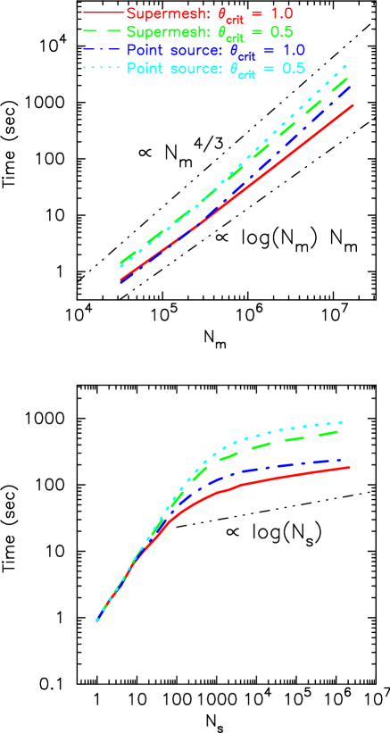
Figure 12: Computation time taken for one step of the RT calculation. Upper panel: Computation time as a function of the number of meshes, $N_{\rm m}$. The number of radiation sources, $N_{\rm s}$ is fixed to 1000. The solid (red) and dashed (green) lines show the results by the supermesh approximation with $\theta_{\rm crit}=1$ and 0.5, respectively. The dot-dashed (blue) and dotted (light blue) lines indicate the point source approximation with $\theta_{\rm crit}=1$ and 0.5, respectively. The thin dot-dot-dot-dashed lines show the scaling with $N_{\rm m}^{4/3}$ and $N_{\rm m}\log(N_{\rm m})$. Lower panel: Same as the upper panel but the number of the source, $N_{\rm s}$, is varied. The number of meshes, $N_{\rm m}$ is fixed to $128^{3}$. The thin dot-dot-dot-dashed line indicates the scaling with $\log(N_{\rm s})$.

4 Summary and discussion

We have presented a code to solve radiative transfer around point sources within a three-dimensional Cartesian grid, ARGOT, which accelerates the RT calculation by utilising the oct-tree structure in order to reduce the effective number of radiation sources. We have explored two methods: one is the supermesh approximation and the other is the point source approximation. In both methods, sources in a tree node whose angular size is smaller than the accuracy parameter $\theta_{\rm crit}$ are treated as a single bright source. As a result, computation time only scales with $\log(N_{\rm s})$. The main difference between these two method is that while the former takes the spatial extent of a source group into account, the latter ignores the size of the source group and treat it as a point source. In the supermesh approximation, the RT is solved using supermeshes whose angular size is similar to the angular size of the source group in question. Doing this results in the further acceleration of the RT calculation.

One might thus see that the supermesh approximation is superior to the point source approximation. We have however shown that the point source approximation is always equally or more accurate than the supermesh approximation for a given value of the accuracy parameter. This is because RT in a inhomogeneous medium on a supermesh inevitably overestimates the optical depth. This approximation can be in principle improved by including higher order moments, such as variance, although we do not take such an approach. This method hence only applicable to the problems in which a local H ii region is driven primarily by one or a few sources such as Test 3 in this paper. When one applies the supermesh method to the simulation of cosmic reionization, it could be combined with the ‘local clumping factor’ approach proposed by Raičević & Theuns (2011), although exploring such a method is beyond the scope of this paper.

The point source approximation, which can be regarded as a mesh version of START (Hasegawa & Umemura, 2010), produces sufficiently accurate results with $\theta_{\rm crit}=1$ for all test simulations presented in this paper. This approximation requires slightly more computational cost than the supermesh approximation and it scales with $N_{\rm m}^{4/3}\log(N_{\rm s})$. The performance can be improved if we choose the angular resolution so that at least one ray from a radiation source (or a group of sources) crosses all target meshes instead of solving RT to all target meshes. Doing this reduces the total number of rays from $\propto N_{\rm m}$ to $\propto N_{\rm m}^{2/3}$. Such an algorithm has been applied for RT from point sources (Yajima et al., 2009) and can be extended to our tree-based algorithm. The expected scaling is $N_{\rm m}\log{N_{\rm s}}$, which is even faster than the supermesh approximation and the same scaling by START.

For parallel implementation, if the entire meshes and sources can fit into memory of one computer node, parallelisation via angle decomposition is preferable to volume decomposition. We implement the angle decomposition by using both MPI and OpenMP. If a simulation size becomes too large to fit into the memory of one computer node, we have to employ the volume decomposition. The volume decomposition for RT around point sources was introduce by Susa (2006) and the algorithm can be applied to our methods. We leave the volume decomposition to future work.

The method presented in this paper can be easily combined with any grid-based hydrodynamic code, even with codes based on AMR (Fryxell et al., 2000; Teyssier, 2002; O’Shea et al., 2004) and will be useful for various astrophysical problems in which a large number of radiation sources are required such as cosmic reionization and galaxy formation. We will apply our code for these issues in a forth coming paper.

References

- Abel et al. (1997) Abel T., Anninos P., Zhang Y., Norman M. L., 1997, New Astron., 2, 181
- Abel et al. (1999) Abel T., Norman M. L., Madau P., 1999, ApJ, 523, 66
- Abel & Wandelt (2002) Abel T., Wandelt B. D., 2002, MNRAS, 330, L53
- Aldrovandi & Pequignot (1973) Aldrovandi S. M. V., Pequignot D., 1973, A&A, 25, 137
- Anninos et al. (1997) Anninos P., Zhang Y., Abel T., Norman M. L., 1997, New Astron., 2, 209
- Aubert & Teyssier (2008) Aubert D., Teyssier R., 2008, MNRAS, 387, 295
- Barnes & Hut (1986) Barnes J., Hut P., 1986, Nat, 324, 446
- Cen (1992) Cen R., 1992, ApJS, 78, 341
- Ciardi et al. (2001) Ciardi B., Ferrara A., Marri S., Raimondo G., 2001, MNRAS, 324, 381
- Fryxell et al. (2000) Fryxell B., et al., 2000, ApJS, 131, 273
- Gnedin & Abel (2001) Gnedin N. Y., Abel T., 2001, New Astron., 6, 437
- González et al. (2007) González M., Audit E., Huynh P., 2007, A&A, 464, 429
- Hasegawa & Umemura (2010) Hasegawa K., Umemura M., 2010, MNRAS, 407, 2632
- Hummer (1994) Hummer D. G., 1994, MNRAS, 268, 109
- Hummer & Storey (1998) Hummer D. G., Storey P. J., 1998, MNRAS, 297, 1073
- Ikeuchi & Ostriker (1986) Ikeuchi S., Ostriker J. P., 1986, ApJ, 301, 522
- Iliev et al. (2006) Iliev I. T., et al., 2006, MNRAS, 371, 1057
- Iliev et al. (2009) —, 2009, MNRAS, 400, 1283
- Janev et al. (1987) Janev R. K., Langer W. D., Evans K., 1987, Elementary processes in Hydrogen-Helium plasmas - Cross sections and reaction rate coefficients, Janev, R. K., Langer, W. D., & Evans, K., ed. Springer
- Krumholz (2006) Krumholz M. R., 2006, ApJL, 641, L45
- Kunasz & Auer (1988) Kunasz P., Auer L. H., 1988, J. Quant. Spectrosc. Radiat. Transfer, 39, 67
- Mellema et al. (1998) Mellema G., Raga A. C., Canto J., Lundqvist P., Balick B., Steffen W., Noriega-Crespo A., 1998, A&A, 331, 335
- Nakamoto et al. (2001) Nakamoto T., Umemura M., Susa H., 2001, MNRAS, 321, 593
- Ohsuga et al. (2005) Ohsuga K., Mori M., Nakamoto T., Mineshige S., 2005, ApJ, 628, 368
- O’Shea et al. (2004) O’Shea B. W., Bryan G., Bordner J., Norman M. L., Abel T., Harkness R., Kritsuk A., 2004, ArXiv Astrophysics e-prints:astro-ph/0403044
- Osterbrock & Ferland (2006) Osterbrock D. E., Ferland G. J., 2006, Astrophysics of gaseous nebulae and active galactic nuclei, 2nd edn., Osterbrock, D. E. & Ferland, G. J., ed. University Science Books
- Pawlik & Schaye (2008) Pawlik A. H., Schaye J., 2008, MNRAS, 389, 651
- Petkova & Springel (2009) Petkova M., Springel V., 2009, MNRAS, 396, 1383
- Petkova & Springel (2011) —, 2011, MNRAS, 415, 3731
- Raičević & Theuns (2011) Raičević M., Theuns T., 2011, MNRAS, 412, L16
- Razoumov & Cardall (2005) Razoumov A. O., Cardall C. Y., 2005, MNRAS, 362, 1413
- Ricotti et al. (2002) Ricotti M., Gnedin N. Y., Shull J. M., 2002, ApJ, 575, 33
- Sokasian et al. (2001) Sokasian A., Abel T., Hernquist L. E., 2001, New Astron., 6, 359
- Stone et al. (1992) Stone J. M., Mihalas D., Norman M. L., 1992, ApJS, 80, 819
- Susa (2006) Susa H., 2006, PASJ, 58, 445
- Teyssier (2002) Teyssier R., 2002, A&A, 385, 337
- Wise & Abel (2011) Wise J. H., Abel T., 2011, MNRAS, 414, 3458
- Yajima et al. (2009) Yajima H., Umemura M., Mori M., Nakamoto T., 2009, MNRAS, 398, 715
- Yoshikawa & Sasaki (2006) Yoshikawa K., Sasaki S., 2006, PASJ, 58, 641