Reducing the Prediction Horizon in NMPC: An Algorithm Based Approach

Abstract

In order to guarantee stability, known results for MPC without additional terminal costs or endpoint constraints often require rather large prediction horizons. Still, stable behavior of closed loop solutions can often be observed even for shorter horizons. Here, we make use of the recent observation that stability can be guaranteed for smaller prediction horizons via Lyapunov arguments if more than only the first control is implemented. Since such a procedure may be harmful in terms of robustness, we derive conditions which allow to increase the rate at which state measurements are used for feedback while maintaining stability and desired performance specifications. Our main contribution consists in developing two algorithms based on the deduced conditions and a corresponding stability theorem which ensures asymptotic stability for the MPC closed loop for significantly shorter prediction horizons.

1 Introduction

Model predictive control (MPC), sometimes also termed receding horizon control (RHC), deals with the problem of approximately solving an infinite horizon optimal control problem which is, in general, computationally intractable. To this end, a solution of the optimal control problem on a truncated, and thus finite, horizon is computed. Then, the first part of the resulting control is implemented at the plant and the finite horizon is shifted forward in time which renders this method to be iteratively applicable, see, e.g., Magni et al. (2009).

During the last decade, theory of MPC has grown rather mature for both linear and nonlinear systems as shown in Allgöwer and Zheng (2000) and Rawlings and Mayne (2009). Additionally, it is used in a variety of industrial applications, cf. Badgwell and Qin (2003) due to its capability to directly incorporate input and state constraints. However, since the original problem is replaced by an iteratively solved sequence of control problems – which are posed on a finite horizon – stability of the resulting closed loop may be lost. In order to ensure stabilty, several modifications of the finite horizon control problems such as stabilizing terminal constraints or a local Lyapunov function as an additional terminal weight have been proposed, cf. Keerthi and Gilbert (1988) and Chen and Allgöwer (1999).

Here, we consider MPC without additional terminal contstraints or costs, which is especially attractive from a computational point of view. Stability for these schemes can be shown via a relaxed Lyapunov inequality, see Grüne (2009) for a set valued framework and Grüne and Pannek (2009) for a trajectory based approach. Still, stable behavior of the MPC controlled closed loop can be observed in many examples even if these theoretical results require a longer prediction horizon in order to guarantee stability. The aim of this paper consists of closing this gap between theory and experimental experience. In particular, we develop an algorithm which enables us to ensure stability for a significantly shorter prediction horizon and, as a consequence, reduces the computational effort in each MPC iteration significantly. The key observation in order to extend the line of arguments in the stability proofs proposed in Grüne (2009) is that the relaxed Lyapunov inequality holds true for the MPC closed loop for smaller horizons if not only the first element but several controls of the open loop are implemented, cf. Grüne et al. (2010). However, this may be harmful in terms of robustness, cf. Magni and Scattolini (2007). Utilizing the internal structure of consecutive MPC problems in the critical cases along the closed loop trajectory, we present conditions which allow us to close the loop more often and maintain stability. Indeed, our results are also applicable in order to deduce performance estimates of the MPC closed loop.

The paper is organized as follows: In Section 2, the MPC problem under consideration is stated. In the ensuing section, we extend suboptimality results from Grüne and Pannek (2009) and Grüne et al. (2010) in order to give a basic MPC algorithm which checks these performance bounds. In Section 4, we develop the proposed algorithm further in order to increase the rate at which state measurements are used for feedback and state our main stability theorem. In the final Section 5 we draw some conclusions. Instead of a separated example, we use a numerical experiment throughout the paper which shows the differences and improvements of the presented result in comparison to known results.

2 Problem formulation

We consider nonlinear discrete time control systems

$$x(n+1)=f(x(n),u(n)),\quad x(0)=x_{0}$$ (1)

with $x(n)\in\mathbb{X}\subset X$ and $u(n)\in\mathbb{U}\subset U$ for $n\in\mathbb{N}_{0}$ where $\mathbb{N}_{0}$ denotes the natural numbers including zero. The state space $X$ and the control value space $U$ are arbitrary metric spaces. As a consequence, the following results are applicable to discrete time dynamics induced by a sampled – finite or infinite dimensional – system, see, e.g., Altmüller et al. (2010) or Ito and Kunisch (2002). Constraints may be incorporated by choosing the sets $\mathbb{X}$ and $\mathbb{U}$ appropriately. Furthermore, we denote the space of control sequences $u:\mathbb{N}_{0}\rightarrow\mathbb{U}$ by $\mathbb{U}^{\mathbb{N}_{0}}$.
Our goal consists of finding a static state feedback $u=\mu(x)\in\mathbb{U}$ which stabilizes a given control system of type (1) at its unique equilibrium $x^{*}$. In order to evaluate the quality of the obtained control sequence, we define the infinite horizon cost functional

$$J_{\infty}(x_{0},u)=\sum\limits_{n=0}^{\infty}\ell(x(n),u(n))$$ (2)

with continuous stage cost $\ell:\mathbb{X}\times\mathbb{U}\rightarrow\mathbb{R}_{0}^{+}$ with $\ell(x^{*},0)=0$ and $\ell(x,u)>0$ for $x\neq x^{*}$. Here, $\mathbb{R}_{0}^{+}$ denotes the nonnegative real numbers. The optimal value function is given by $V_{\infty}(x_{0})=\inf_{u\in\mathbb{U}^{\mathbb{N}_{0}}}J_{\infty}(x_{0},u)$ and, for the sake of convenience, it is assumed that the infimum with respect to $u\in\mathbb{U}^{\mathbb{N}_{0}}$ is attained. Based on the optimal value function $V_{\infty}(\cdot)$, an optimal feedback law on the infinite horizon can be defined as

$$\mu_{\infty}(x(n)):=\mathop{\rm argmin}_{u\in\mathbb{U}}\left\{V_{\infty}(x(n+1))+\ell(x(n),u)\right\}$$ (3)

using Bellman’s principle of optimality. However, since the computation of the desired control law (3) requires, in general, the solution of a Hamilton–Jacobi–Bellman equation, which is very hard to solve, we use a model predictive control (MPC) approach instead. The fundamental idea of MPC consists of three steps which are repeated at every discrete time instant:

• Firstly, an optimal control $(u_{0}^{\star},u_{1}^{\star},\ldots,u_{N-1}^{\star})\in\mathbb{U}^{N}$ for the problem on a finite horizon $[0,N)$, i.e.,

  $$J_{N}(x_{0},u)=\sum\limits_{k=0}^{N-1}\ell(x_{u}(k;x_{0}),u(k))$$ (4)

  is computed given the most recent known state $x_{0}$ of the system (1). Here, $x_{u}(\cdot;x_{0})$ corresponds to the open loop trajectory of the prediction with control $u$ and initial state $x_{0}$.

• Secondly, the first element $\mu_{N}(x_{0})=u_{0}^{\star}$ of the obtained sequence of open loop control values is implemented at the plant.

• Thirdly, the entire optimal control problem considered in the first step is shifted forward in time by one discrete time instant which allows for an iterative application of this procedure.

The corresponding closed loop costs are given by

$$J_{\infty}(x_{0},\mu_{N})=\sum\limits_{n=0}^{\infty}\ell(x_{\mu_{N}}(n),\mu_{N}(x_{\mu_{N}}(n)))$$

where $x_{\mu_{N}}(\cdot)$ denotes the closed loop solution. We use

$$u_{N}(\cdot;x_{0})=\mathop{\rm argmin}_{u\in\mathbb{U}^{N}}J_{N}(x_{0},u)$$ (5)

to abbreviate the minimizing open loop control sequence and $V_{N}(x_{0})=\min_{u\in\mathbb{U}^{N}}J_{N}(x_{0},u)$ for the corresponding optimal value function. Furthermore, we say that a continuous function $\rho:\mathbb{R}_{\geq 0}\rightarrow\mathbb{R}_{\geq 0}$ is of class $\mathcal{K}_{\infty}$ if it satisfies $\rho(0)=0$, is strictly increasing and unbounded, and a continuous function $\beta:\mathbb{R}_{\geq 0}\times\mathbb{R}_{\geq 0}\rightarrow\mathbb{R}_{\geq 0}$ is of class $\mathcal{KL}$ if it is strictly decreasing in its second argument with $\lim_{t\rightarrow\infty}\beta(r,t)=0$ for each $r>0$ and satisfies $\beta(\cdot,t)\in\mathcal{K}_{\infty}$ for each $t\geq 0$.

Note that, different to the infinite horizon problem (2), the first step of the MPC problem consists of minimizing the truncated cost functional (4) over a finite horizon. While commonly endpoint constraints or a Lyapunov function type endpoint weight are used to ensure stability of the closed loop, see, e.g., Keerthi and Gilbert (1988), Chen and Allgöwer (1999), Jadbabaie and Hauser (2005) and Graichen and Kugi (2010), we consider the plain MPC version without these modifications. According to Grüne and Pannek (2009), stable behavior of the closed loop trajectory can be guaranteed using relaxed dynamic programming.

Proposition 2.1

(i) Consider the feedback law $\mu_{N}:\mathbb{X}\rightarrow\mathbb{U}$ and the closed loop trajectory $x_{\mu_{N}}(\cdot)$ with initial value $x(0)=x_{0}\in\mathbb{X}$. If

$$V_{N}(x_{\mu_{N}}(n))\geq V_{N}(x_{\mu_{N}}(n+1))+\alpha\ell(x_{\mu_{N}}(n),\mu_{N}(x(n)))$$ (6)

holds for some $\alpha\in(0,1]$ and all $n\in\mathbb{N}_{0}$, then

$$\alpha V_{\infty}(x_{0})\leq\alpha J_{\infty}(x_{0},\mu_{N})\leq V_{N}(x_{0})\leq V_{\infty}(x_{0})$$ (7)

holds.
(ii) If, in addition, there exist $\alpha_{1},\alpha_{2},\alpha_{3}\in\mathcal{K}_{\infty}$ such that $\alpha_{1}(\|x\|)\leq V_{N}(x)\leq\alpha_{2}(\|x\|)$ and $\ell(x,u)\geq\alpha_{3}(\|x\|)$ hold for all $x=x_{\mu_{N}}(n)\in\mathbb{X}$, $n\in\mathbb{N}_{0}$, then there exists $\beta\in\mathcal{KL}$ which only depends on $\alpha_{1},\alpha_{2},\alpha_{3}$ and $\alpha$ such that the inequality $\|x_{\mu_{N}}(n)\|\leq\beta(\|x_{0}\|,n)$ holds for all $n\in\mathbb{N}_{0}$, i.e., $x_{\mu_{N}}(\cdot)$ behaves like a trajectory of an asymptotically stable system.

The key assumption in Proposition 2.1 is the relaxed Lyapunov–inequality (6) in which $\alpha$ can be interpreted as a lower bound for the rate of convergence. From the literature, it is well–known that this condition is satisfied for sufficiently long horizons $N$, cf. Jadbabaie and Hauser (2005), Grimm et al. (2005) or Alamir and Bornard (1995), and that a suitable $N$ may be computed via methods described in Pannek (2009). To investigate whether this condition is restrictive, we consider the following example.

Example 2.2

Consider the synchronous generator model

$$\dot{x}_{1}(t) =x_{2}(t)$$

$$\dot{x}_{2}(t) =-b_{1}x_{3}(t)\sin x_{1}(t)-b_{2}x_{2}(t)+P$$

$$\dot{x}_{3}(t) =b_{3}\cos x_{1}(t)-b_{4}x_{3}(t)+E+u(t)$$

with parameters $b_{1}=34.29$, $b_{2}=0.0$, $b_{3}=0.149$, $b_{4}=0.3341$, $P=28.22$, and $E=0.2405$ from Galaz et al. (2003) and the initial value $x_{0}=(1.02,0.1,1.014)$.

For Example 2.2 our aim is to steer the system to its equilibrium $x^{*}\approx(1.12,0.0,0.914)$. To this end, we use MPC to generate results for sampling time $T=0.1$ and running cost

$$\ell(x,u)=\int_{0}^{T}\|\varphi(t;x,\tilde{u})-x^{*}\|^{2}+\lambda\|\tilde{u}(t)\|^{2}\,dt$$

with piecewise constant control $\tilde{u}(t)=u$ for $t\in[0,T)$ and $\lambda=10^{-6}$ where $\varphi(\cdot;x,\tilde{u})$ denotes the solution operator of the differential equation with initial value $x$ and control $\tilde{u}$. For this setting, we obtain stability of the closed loop via inequality (6) for $N\geq 30$, cf. Figure 1. However, Figure 1 shows stable behavior of the closed loop for the smaller prediction horizon $N=19$ without significant deviations – despite the fact that the relaxed Lyapunov–inequality from Proposition 2.1 is violated at three instances.

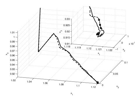
Figure 1: Comparison of closed loop solutions for $N=30$ (solid) and $N=19$ (dashed) where $(\square)$ marks a violation of the suboptimality bound $\overline{\alpha}=0.1$

Our numerical experiment shows that, even if stability and the desired performance estimate (7) cannot be guaranteed via Proposition 2.1, stable and satisfactory behavior of the closed loop may still be observed. Hence, since the computational effort grows rapidly with respect to the prediction horizon, our goal consists of developing an algorithm which allows for significantly reducing the prediction horizon. To this end, we adapt the thereotical condition given in (6). Moreover, the proposed algorithms check – at runtime – whether these conditions are satisfied or not.

Note that, since we do not impose additional stabilizing terminal constraints, feasibility of the NMPC scheme is an issue that cannot be neglected. In particular, without these stabilizing constraints the closed loop trajectory might run into a dead end. To exclude such a scenario, we assume the following viability condition to hold.

Assumption 2.3

For each $x\in\mathbb{X}$ there exists a control $u\in\mathbb{U}$ such that $f(x,u)\in\mathbb{X}$ holds.

3 Theoretical Background

In Section 2 we observed a mismatch between the relaxed Lyapunov inequality (6) and the results from Example 2.2 which indicates that the closed loop exhibits a stable and – in terms of performance – satisfactory behavior for significantly smaller prediction horizons $N$. In Grüne et al. (2010) it has been shown that the suboptimality estimate $\alpha$ is increasing (up to a certain point) if more than one element of the computed sequence of control values is applied. Hence, we vary the number of open loop control values to be implemented during runtime at each MPC iteration, i.e., the system may stay in open loop for more than one sampling period, in order to deal with this issue. Doing so, however, may lead to severe problems, e.g., in terms of robustness, cf. Magni and Scattolini (2007). Hence, the central aim of this work is the development of an algorithm which checks – at runtime – whether it is necessary to remain in open loop in order to guarantee the desired stability behavior of the closed loop by suboptimality arguments, or if the loop can be closed without loosing these characteristics.

To this end, we introduce the list $\mathcal{S}=(s(0),s(1),\ldots)\subseteq\mathbb{N}_{0}$, which we assume to be in ascending order, in order to indicate time instances at which the control sequence is updated. Moreover, we denote the closed loop solution at time instant $s(n)$ by $x_{n}=x_{\mu_{N}}(s(n))$ and define $m_{n}:=s(n+1)-s(n)$, i.e., the time between two MPC updates. Hence,

$$x_{\mu_{N}}(s(n)+m_{n})=x_{\mu_{N}}(s(n+1))=x_{n+1}$$

holds. This enables us – in view of Bellman’s principle of optimality – to define the closed loop control

$$\mu_{N}^{\mathcal{S}}(\cdot;x_{n}) :=\mathop{\rm argmin}_{u\in\mathbb{U}^{m_{n}}}\Big{\{}V_{N-m_{n}}(x_{u}(m_{n};x_{n}))$$ (8)

$$\qquad\qquad\quad+\sum\limits_{k=0}^{m_{n}-1}\ell(x_{u}(k;x_{n}),u(k))\Big{\}}.$$

In Grüne et al. (2010), a suboptimality degree $\alpha_{N,m_{n}}$ relative to the horizon length $N$ and the number of controls to be implemented $m_{n}$ has been introduced in order to measure the tradeoff between the infinite horizon cost induced by the MPC feedback law $\mu_{N}^{\mathcal{S}}(\cdot;\cdot)$, i.e.

$$V_{\infty}^{\mu_{N}^{\mathcal{S}}}(x_{0}):=\sum\limits_{n=0}^{\infty}\sum\limits_{k=0}^{m_{n}-1}\ell\left(x_{\mu_{N}^{\mathcal{S}}}(k;x_{n}),\mu_{N}^{\mathcal{S}}(k;x_{n})\right),$$ (9)

and the infinite horizon optimal value function $V_{\infty}(\cdot)$. In particular, it has been shown that given a controllability condition, i.e., for each $x_{0}$ there exists a control $u_{x_{0}}$ such that

$$\ell(x_{u_{x_{0}}}(n;x_{0}),u_{x_{0}}(n;x_{0}))\leq C\sigma^{n}\min_{u\in\mathbb{U}}\ell(x_{0},u)$$ (10)

holds with $C\geq 1$, $\sigma\in(0,1)$, then there exists a prediction horizon $N\in\mathbb{N}_{\geq 2}$ and $\overline{m}\in\{1,\ldots,\lfloor N/2\rfloor\}$ such that $\alpha_{N,\overline{m}}\geq\overline{\alpha}$ for an arbitrarily specified $\overline{\alpha}\in(0,1)$.

Example 3.1

Suppose (10) to hold with $C=4$ and $\sigma=0.6$ and fix $\overline{\alpha}=0.275$. Then the pair $(N,\overline{m})=(15,6)$ implies $\alpha_{N,\overline{m}}\approx 0.294>\overline{\alpha}$, cf. Figure 2, i.e., the closed–loop satisfies the performance bound $\overline{\alpha}$. However, $N=25$ is the smallest prediction horizon which yields $\alpha_{N,m}\geq\overline{\alpha}$ for $m=1$, i.e., classical MPC, cf. Figure 3.

Figure 2: Visualization of the $\alpha_{15,\cdot}$-values with respect to the number of controls to be implemented $m=1,\ldots,\lfloor N/2\rfloor\}$ for prediction horizon $N=15$. The dashed line indicates the reference value $\overline{\alpha}=0.275$.

Examples 3.1 shows that choosing a larger value for $m$ may significantly reduce the required prediction horizon length and, consequently, the numerical effort which grows rapidly with respect to the horizon $N$.

Since the shape of the curve in Figure 2 is not a coincidence, i.e., $\alpha_{N,\lfloor N/2\rfloor}\geq\alpha_{N,m}$ holds for $m\in\{1,\ldots,N-1\}$, cf. Grüne et al. (2010), we may easily determine the smallest prediction horizon $N\in\mathbb{N}_{\geq 2}$ such that $\alpha_{N,\lfloor N/2\rfloor}\geq\overline{\alpha}$ ensures the desired performance specification.

Figure 3: Illustration of the $\alpha_{\cdot,1}$-values with respect to the prediction horizon $N\in\{15,\ldots,25\}$ for $m=1$, i.e., classical MPC. The dashed line indicates the reference value $\overline{\alpha}=0.275$.

However, note that these results exhibit a set–valued nature. Hence, the validity of the controllability condition (10) and the use of a prediction horizon length corresponding to the mentioned formula lead to an estimate which may be conservative – at least in parts of the state space. This motivates the development of algorithms which use the above calculated horizon length but close the control loop more often. Here, we make use of an extension of the $m$-step suboptimality estimate derived in Grüne and Pannek (2009) which is similar to Grüne et al. (2010) but can be applied in a trajectory based setting.

Proposition 3.2

Consider $\overline{\alpha}\in(0,1]$ to be fixed. If there exists a function $V_{N}:\mathbb{X}\rightarrow\mathbb{R}_{0}^{+}$ satisfying

$$V_{N}(x_{n})\geq V_{N}(x_{n+1})+\overline{\alpha}\sum\limits_{k=0}^{m_{n}-1}\ell(x_{u_{N}}(k;x_{n}),u_{N}(k;x_{n}))$$ (11)

with $m_{n}\in\{1,\ldots,N-1\}$ for all $n\in\mathbb{N}_{0}$, then

$$V_{\infty}^{\mu_{N}^{\mathcal{S}}}(x_{0})\leq\frac{1}{\overline{\alpha}}\cdot V_{\infty}(x_{0})$$ (12)

holds for all $n\in\mathbb{N}_{0}$.

Proof: Reordering (11), we obtain

$$\overline{\alpha}\sum\limits_{k=0}^{m_{n}-1}\ell(x_{u_{N}}(k;x_{n}),u_{N}(k;x_{n}))\leq V_{N}(x_{n})-V_{N}(x_{n+1}).$$

Summing over $n\in\mathbb{N}_{0}$ yields

$$\overline{\alpha}\sum\limits_{i=0}^{n}\sum\limits_{k=0}^{m_{i}-1}\ell(x_{u_{N}}(k;x_{i}),u_{N}(k;x_{i}))$$

$$\leq V_{N}(x_{0})-V_{N}(x_{n+1})\leq V_{N}(x_{0})$$

and hence taking $n$ to infinity implies the assertion.∎

Remark 3.3

Note that the assumptions of Proposition 3.2 indeed imply the estimate

$$V_{\infty}(x_{n})\leq V_{\infty}^{\mu_{N}^{\mathcal{S}}}(x_{n})\leq\frac{1}{\overline{\alpha}}V_{\infty}(x_{n})$$ (13)

for all $n\in\mathbb{N}_{0}$ which can be proven analogously.

Note that $\mathcal{S}$ is built up during runtime of the algorithm and not known in advance. Hence, $\mathcal{S}$ is always ordered. A corresponding implementation which aims at guaranteeing a fixed lower bound of the degree of suboptimality $\overline{\alpha}$ takes the following form: Given state $x:=x_{0}$, list $\mathcal{S}=(0)$, $N\in\mathbb{N}_{\geq 2}$, and $\overline{\alpha}\in(0,1)$

• Set $j=0$, compute $u_{N}(\cdot;x)$ and $V_{N}(x)$. Do

  • Set $j=j+1$, compute $V_{N}(x_{u_{N}}(j;x))$

  • Compute maximal $\alpha$ to satisfy (11)

  • If $\alpha\geq\overline{\alpha}$: Set $m_{n}=j$ and goto 2

  • If $j=N-1$: Print warning “Solution may diverge”, set $m_{n}=1$ and goto 2

  while $\alpha<\overline{\alpha}$

• For $j=1,\ldots,m_{n}$ do

  • Implement $\mu_{N}^{\mathcal{S}}(j-1;x):=u_{N}(j-1;x)$

• Set $\mathcal{S}:=(\mathcal{S},\text{back}(\mathcal{S})+m_{n})$, $x:=x_{\mu_{N}^{\mathcal{S}}}(m_{n};x)$, goto 1

Remark 3.4

Here, we adopted the programming notation back which allows for fast access to the last element of a list.

Remark 3.5

If (11) is not satisfied for $j\leq N-1$, a warning will be printed out because the performance bound $\overline{\alpha}$ cannot be guaranteed. In order to cope with this issue, there exist remedies, e.g., one may increase the prediction horizon and repeat step 1. For sufficiently large $N$, this ensures the local validity of (11). Unfortunately, the proof of Proposition 3.2 cannot be applied in this context due to the prolongation of the horizon. Yet, it can be replaced by estimates from Pannek (2009) or Giselsson (2010) for varying prediction horizons to obtain a result similar to (12). Alternatively, one may continue with the algorithm. If there does not occur another warning, the algorithm guarantees the desired performance for $x_{n}$ instead of $x_{0}$, i.e., from that point on, cf. Remark 3.3.

In order to obtain a robust procedure, however, it is preferable that the control loop is closed as often as possible, i.e., $m_{n}=1$ for all $n\in\mathbb{N}_{0}$. In the following section, we give results and corresponding algorithms which – given certain conditions – allow us to reduce $m_{n}$.

4 Algorithms and Stability Results

In many applications a stable behavior of the closed loop is observed for $m_{n}=1$ even if it cannot be guaranteed using the suboptimality estimate (6), cf. Example 2.2. Here, we present a methodology to close the control loop more often while maintaining stability. In particular, if $m_{n}>1$ is required in order to ensure $\alpha\geq\overline{\alpha}$ in (11) and, as a consequence, in step (1) of the proposed algorithm, we present conditions which allow us to update the control for some $j\in\{1,\ldots,m_{n}-1\}$ to

$$\hat{u}_{N}(k;x_{n}):=\begin{cases}u_{N}(k;x_{n}),&k\leq j-1\\ u_{N}(k-j;x_{u_{N}}(j;x_{n})),&k\geq j\end{cases}$$ (14)

insert the new updating time instant $s(n)+j$ into the list $\mathcal{S}$, and still be able to guarantee the desired stability behavior of the closed loop. Summarizing, our aim consists of guaranteeing that the degree of suboptimality $\overline{\alpha}$ is maintained, i.e., (11) is still satisfied, for the MPC law updated at a time instant $j\leq m_{n}-1$ according to (14).

Proposition 4.1

Let $x_{n}\in\mathbb{X}$ be given and inequality (11) hold for $u_{N}(\cdot;x_{n})$, $\overline{\alpha}>0$, and $m_{n}\in\{2,\ldots,N-1\}$. If the inequality

$$V_{N}(x_{u_{N}}(m_{n}-j;x_{u_{N}}(j;x_{n})))-V_{N-j}(x_{u_{N}}(j;x_{n}))$$

$$\leq(1-\overline{\alpha})\sum\limits_{k=0}^{j-1}\ell(x_{u_{N}}(k;x_{n}),u_{N}(k;x_{n}))$$ (15)

$$-\overline{\alpha}\sum\limits_{k=j}^{m_{n}-1}\ell(x_{u_{N}}(k-j;x_{u_{N}}(j;x_{n})),u_{N}(k-j;x_{u_{N}}(j;x_{n})))$$

holds for some $j\in\{1,\ldots,m_{n}-1\}$, then the control sequence $u_{N}(\cdot;x_{n})$ can be replaced by (14) and suboptimality degree $\overline{\alpha}$ is locally maintained.

Proof: In order to show the assertion, we need to show (11) for the modified control sequence (14). Reformulating (15) by shifting the running costs associated with the unchanged control to the left hand side of (15) we obtain

$$V_{N}(x_{u_{N}}(m_{n}-j;x_{u_{N}}(j;x_{n})))-V_{N}(x_{u_{N}}(0;x_{n}))$$

$$\qquad\qquad\leq-\overline{\alpha}\sum\limits_{k=0}^{m_{n}-1}\ell(x_{\hat{u}_{N}}(k;x_{n}),\hat{u}_{N}(k;x_{n}))$$

which is equivalent to

$$V_{N}(x_{n}) \geq V_{N}(x_{\hat{u}_{N}}(m_{n};x_{n}))$$

$$+\overline{\alpha}\sum\limits_{k=0}^{m_{n}-1}\ell(x_{\hat{u}_{N}}(k;x_{n}),\hat{u}_{N}(k;x_{n})),$$

i.e., the relaxed Lyapunov inequality (11) for the updated control $\hat{u}_{N}(\cdot;x_{n})$.∎

Example 4.2

Consider the illustrative Example 2.2 with horizon $N=19$ and $\overline{\alpha}=0.1$. For this setting, we obtain $\alpha\geq\overline{\alpha}$ with $m_{n}=1$ for all updating instances $s_{n}\in\mathcal{S}$ except for those three points indicated by $(\square)$ in Figure 1 where we have $m_{n}=2$ once and $m_{n}=3$ twice. Yet, for each of these points, inequality (15) holds with $j=1$.

• $m_{n}=2$: We apply Theorem 4.1 in order to update the control $u_{N}(\cdot;x_{n}):=\hat{u}_{N}(\cdot;x)$ according to (14). Thus, since the MPC law was updated at each sampling instant, we have obtained stability of the classical MPC closed loop.

• $m_{n}=3$: We utilize Theorem 4.1 in an iterative manner: since (15) holds for $j=1$, we proceed as in the case $m_{n}=2$, update the control $u_{N}(\cdot;x_{n}):=\hat{u}_{N}(\cdot;x_{n})$, and compute $x_{\mu_{N}}(2;x_{n})$. Then, we compute $u_{N}(\cdot;x_{\mu_{N}}(2;x_{n}))$ and check whether or not (15) holds for (14) with $j=2$. Note that here, $u_{N}(\cdot;x_{n})$ in (14) is already an updated control sequence. Since (15) holds true, we obtain stability of the closed loop for the updated MPC control sequence. Moreover, we applied $\mu_{N}(x(s(n))$, $\mu_{N}(x(s(n)+1))$ and $\mu_{N}(x(s(n)+2))$ instead of $\mu_{N}^{\mathcal{S}}(i;x(s(n)))$, $i=0,1,2$, i.e., we have again used classical MPC.

Note that this iterative procedure can be extended in a similar manner for all $m_{n}\leq N-1$.

Integrating the results from Theorem 4.1 into the algorithm displayed after Proposition 3.2 can be done by changing Step (2).

• For $j=1,\ldots,m_{n}$ do

  • Implement $\mu_{N}^{\mathcal{S}}(j-1;x):=u_{N}(j-1;x)$

  • Compute $u_{N}(\cdot;x_{u_{N}}(j;x))$ and $V_{N}(x_{\hat{u}_{N}}(m_{n};x))$

  • If $j<m_{n}$ and condition (15) holds:

    • Construct $\hat{u}_{N}(\cdot;x)$ according to (14)

    • Update $u_{N}(\cdot;x):=\hat{u}_{N}(\cdot;x)$

Note that $V_{N-j}(x_{u_{N}}(j;x_{n}))$ in (15) is known in advance from $V_{N}(x_{n})$ due to the principle of optimality. Hence, only $u_{N}(\cdot;x_{u_{N}}(j;x_{n}))$ and $V_{N}(x_{\hat{u}_{n}}(m_{n};x_{n}))$ need to be computed. Unfortunately, this result has to be checked for all $j\in\{1,\ldots,m_{n}-2\}$ using the comparison basis $V_{N}(x_{n})$. As a consequence, we always have to keep the updating instant $s(n)$ in mind, cf. Example 4.2. The following result allows us to weaken this restriction:

Proposition 4.3

Let $x_{n}\in\mathbb{X}$ be given and inequality (11) hold for $u_{N}(\cdot;x_{n})$, $\overline{\alpha}>0$, and $m_{n}\in\{2,\ldots,N-1\}$. If the inequality

$$V_{N}(x_{u_{N}}(m_{n}-j;x_{u_{N}}(j;x_{n})))-V_{N}(x_{u_{N}}(m_{n};x_{n}))$$

$$\leq\overline{\alpha}\sum\limits_{k=j}^{m_{n}-1}\big{(}\ell(x_{u_{N}}(k;x_{n}),u_{N}(k;x_{n}))$$ (17)

$$\qquad-\ell(x_{u_{N}}(k-j;x_{u_{N}}(j;x_{n})),u_{N}(k-j;x_{u_{N}}(j;x_{n})))\big{)}$$

holds for some $j\in\{1,\ldots,m_{n}-1\}$, then the control sequence $u_{N}(\cdot;x_{n})$ can be replaced by (14) and suboptimality degree $\alpha$ is locally maintained.

Proof: Adding (17) to (11) leads to

$$V_{N}(x_{\hat{u}_{N}}(m_{n};x_{n}))-V_{N}(x_{n})$$

$$\qquad\qquad\leq-\overline{\alpha}\sum\limits_{k=0}^{j-1}\ell(x_{u_{N}}(k;x_{n}),u_{N}(k;x_{n}))$$

$$\qquad\qquad\quad-\overline{\alpha}\sum\limits_{k=j}^{m_{n}-1}\ell(x_{\hat{u}_{N}}(k;x_{n}),\hat{u}_{N}(k;x_{n})).$$

Updating the control sequence according to (14), we obtain (4) which completes the proof.∎

Remark 4.4

We also like to point out that conditions (15) and (17) allow for a less fast decrease of energy along the closed loop, i.e., the case $V_{N}(x_{\hat{u}_{N}}(m_{n};x_{n}))\geq V_{N}(x_{u_{N}}(m_{n};x_{n}))$ is not excluded in general.

As outlined in Example 4.2, Theorem 4.1 (and analogously Theorem 4.3) may be applied iteratively. Yet, in contrast to (15), $V_{N}(x_{n})$ is not required in (17). Hence, if an appropriate update can be found for time instant $j\in\{1,\ldots,m_{n}-1\}$, the loop can be closed and, as a consequence, Theorem 4.3 can be applied to the new initial value $x_{\hat{u}}(j;x_{n})$ with respect to the reduced number of control to be implemented $m_{n}-j$. To this end, the following modification of Step (2c) can be used:

• If $j<m_{n}$ and condition (17) holds:

  • Construct $\hat{u}_{N}(\cdot;x)$ according to (14)

  • Update $u_{N}(\cdot;x):=\hat{u}_{N}(\cdot;x)$

  • Update the values $V_{N}(x_{u_{N}}(m_{n};x))$ and
    $\ell(x_{u_{N}}(k;x),u_{N}(k;x))$, $k=j,\ldots,m_{n}-1$

Combining the results from Proposition 3.2 and Theorems 4.1, 4.3, we obtain our main stability result:

Theorem 4.5

Let $x_{0}\in\mathbb{X}$, $\overline{\alpha}>0$ be given and apply one of the three proposed algorithms. Assume that (1c) is satisfied for some $j\in\{1,\ldots,N-1\}$ for each iterate. Then the closed loop trajectory satisfies the performance estimate (12) from Proposition 3.2. If, in addition, the conditions of Proposition 2.1(ii) hold, then $x_{\mu_{N}}(\cdot)$ behaves like a trajectory of an asymptotically stable system.

Proof: The algorithms construct the set $\mathcal{S}$. Since (1c) is satisfied for some $j\in\{1,\ldots,N-1\}$ the assumptions of Proposition 3.2, i.e., inequality (11) for $x_{n}=x_{\mu_{N}}(s(n))$, are satisfied which implies (12). To conclude asymptotically stable behavior of the closed loop, standard direct Lyapunov techniques can be applied. ∎

Example 4.6

Again consider Example 2.2 with $N=19$ and $\overline{\alpha}=0.1$. Since (17) is more conservative than (15), the closed loop control and accordingly the closed loop solution $x_{\mu_{N}}(\cdot)$ will not coincide in general. This also holds true in our example: While the case $m_{n}=2$ can be resolved similarly using the algorithm based on (17), no update of the control $u_{N}$ is performed for the two cases $m_{n}=3$. Here, this does not cause any change in the list $\mathcal{S}$. However, in general, $\mathcal{S}$ is likely to be different for the presented algorithms.

Since the proposed algorithms guarantee stability for the significantly smaller horizon $N=19$, the computing time for Example 2.2 is reduced by almost $50\%$ – despite the additional computational effort for Step (2).

5 Conclusion

Based on a detailed analysis of a relaxed Lyapunov inequality, we have deduced conditions in order to close the gap between theoretical stability results and stable behavior of the MPC closed loop. Using this additional insight, we developed two MPC algorithms which check these conditions at runtime. Although the additional computational effort is not negligible, the proposed algorithms may allow us to shorten the prediction horizon used in the optimization. This reduces, in general, the complexity of the problem significantly which may imply a reduction of the overall computational costs.

References

- Alamir and Bornard (1995) Alamir, M. and Bornard, G. (1995). Stability of a truncated infinite constrained receding horizon scheme: the general discrete nonlinear case. Automatica, 31(9), 1353–1356.
- Allgöwer and Zheng (2000) Allgöwer, F. and Zheng, A. (2000). Nonlinear model predictive control, volume 26 of Progress in Systems and Control Theory. Birkhäuser Verlag, Basel. Papers from the workshop held in Ascona, June 2–6, 1998.
- Altmüller et al. (2010) Altmüller, N., Grüne, L., and Worthmann, K. (2010). Receding horizon optimal control for the wave equation. In Proceedings of the 49th IEEE Conference on Decision and Control, 3427–3432. Atlanta, Georgia.
- Badgwell and Qin (2003) Badgwell, T. and Qin, S. (2003). A survey of industrial model predictive control technology. Control Engineering Practice, 11, 733–764.
- Chen and Allgöwer (1999) Chen, H. and Allgöwer, F. (1999). Nonlinear model predictive control schemes with guaranteed stability. In Nonlinear Model Based Process Control, 465–494. Kluwer Academic Publishers, Dodrecht.
- Galaz et al. (2003) Galaz, M., Ortega, R., Bazanella, A., and Stankovic, A. (2003). An energy-shaping approach to the design of excitation control of synchronous generators. Automatica J. IFAC, 39(1), 111–119.
- Giselsson (2010) Giselsson, P. (2010). Adaptive Nonlinear Model Predictive Control with Suboptimality and Stability Guarantees. In Proceedings of the 49th Conference on Decision and Control, 3644–3649. Atlanta, GA.
- Graichen and Kugi (2010) Graichen, K. and Kugi, A. (2010). Stability and incremental improvement of suboptimal MPC without terminal constraints. IEEE Trans. Automat. Control. To appear.
- Grimm et al. (2005) Grimm, G., Messina, M., Tuna, S., and Teel, A. (2005). Model predictive control: for want of a local control Lyapunov function, all is not lost. IEEE Trans. Automat. Control, 50(5), 546–558.
- Grüne (2009) Grüne, L. (2009). Analysis and design of unconstrained nonlinear MPC schemes for finite and infinite dimensional systems. SIAM Journal on Control and Optimization, 48, 1206–1228.
- Grüne and Pannek (2009) Grüne, L. and Pannek, J. (2009). Practical NMPC suboptimality estimates along trajectories. Sys. & Contr. Lett., 58(3), 161–168.
- Grüne et al. (2010) Grüne, L., Pannek, J., Seehafer, M., and Worthmann, K. (2010). Analysis of unconstrained nonlinear MPC schemes with varying control horizon. SIAM J. Control Optim., 48(8), 4938–4962.
- Ito and Kunisch (2002) Ito, K. and Kunisch, K. (2002). Receding horizon optimal control for infinite dimensional systems. ESAIM Control Optim. Calc. Var., 8, 741–760.
- Jadbabaie and Hauser (2005) Jadbabaie, A. and Hauser, J. (2005). On the stability of receding horizon control with a general terminal cost. IEEE Trans. Automat. Control, 50(5), 674–678.
- Keerthi and Gilbert (1988) Keerthi, S. and Gilbert, E. (1988). Optimal infinite-horizon feedback laws for a general class of constrained discrete-time systems: stability and moving-horizon approximations. J. Optim. Theory Appl., 57(2), 265–293.
- Magni et al. (2009) Magni, L., Raimondo, D., and Allgöwer, F. (2009). Nonlinear model predictive control. Towards new challenging applications. Springer Berlin.
- Magni and Scattolini (2007) Magni, L. and Scattolini, R. (2007). Robustness and robust design of MPC for nonlinear discrete-time systems. In R. Findeisen, F. Allgöwer, and L.T. Biegler (eds.), Assessment and future directions of nonlinear model predictive control, volume 358 of Lecture Notes in Control and Inform. Sci., 239–254. Springer, Berlin.
- Pannek (2009) Pannek, J. (2009). Receding Horizon Control: A Suboptimality–based Approach. PhD–Thesis in Mathematics, University of Bayreuth, Germany.
- Rawlings and Mayne (2009) Rawlings, J.B. and Mayne, D.Q. (2009). Model Predictive Control: Theory and Design. Nob Hill Publishing, Madison.