A simple toy model for a unified picture of dark energy, dark matter, and inflation

Abstract

A specific scale factor in Robertson-Walker metric with the prospect of giving the overall cosmic history in a unified picture roughly is considered. The corresponding energy-momentum tensor is identified as that of two scalar fields where one plays the roles of both inflaton and dark matter while the other accounts for dark energy. A preliminary phenomenological analysis gives an order of magnitude agreement with observational data. The resulting picture may be considered as a first step towards a single model for all epochs of cosmic evolution.

I introduction

There is an intense on-going research to understand the natures of late-time acceleration PDG (whose standard explanation is dark-energy dark-energy ), dark-matter dark-matter , and the inflationary era inflation1 ; inflation2 . A detailed and definite formulation of each of these issues by its own is essential and very important for the future direction of cosmology. However how to relate these in a single formulation and unify ally eras of cosmology (namely, inflationary, radiation dominated, matter dominated, the current late-time acceleration) is as essential as the study of each era separately. This is not only due to the fact that we must eventually put all these into single picture but it is necessary for a better and correct formulation each of these issues. This paper is an attempt in this direction i.e. to obtain an overall picture of cosmic history in a single model. Some of the other studies in this direction may be found in Guendelman ; Sola ; others . I hope the study given here is simpler and more concrete while being minimal and formulated in standard framework i.e. two standard scalar fields in the usual 4-dimensional Robertson Walker metric and the usual Einstein-Hilbert gravity.

In this paper I consider a specific scale factor in the usual 4-dimensional Robertson-Walker metric. The scale factor is chosen in a such a way that it has a prospect to account for inflationary, matter dominated, and late-time acceleration eras of the universe. Then I check this expectation. First I find the corresponding energy-momentum tensor and identify it by that of two scalar fields. The first one mimics inflation at very small times and then mimics (dark) matter at intermediate times. The second one is identified by dark energy. Hence this model accounts for all epochs of the universe except the radiation dominated one. The content of this universe is similar to our own except it does not contain baryonic matter and radiation. This universe is similar to our own, given the fact that the present ratio of baryonic matter density and radiation to the total energy density of the universe is 4 $\%$ and hence negligible and remains negligible (at gravitational level) in most of the cosmological evolution except in the radiation dominated era. Then I use cosmological data to constraint the parameters of the model and apply these to some redshifts and to the corresponding time data to check the phenomenological viability of the model. There is an order of magnitude agreement with data. In my opinion the results are encouraging to look for a more elaborate form of the model where baryonic matter and radiation are included, and where a more thorough study of the parameter space is investigated.

II the model

We consider the Robertson-Walker metric

$$ds^{2}\;=\;g_{\mu\nu}dx^{\mu}\,dx^{\nu}\,=\,-dt^{2}\,+\,a^{2}(t)\tilde{g}_{ij}dx^{i}dx^{j}$$ (1)

We take the 3-dimensional space be flat, i.e. $\tilde{g}_{ij}=\delta_{ij}$ for the sake of simplicity, which is an assumption consistent with cosmological observations PDG . The key assumption in this paper is the following ansatz

$$a(t)\,=\,[p_{1}\,+\,p_{2}a_{2}t]\,Exp[-b_{1}(a_{2}t)^{-1/6}]$$ (2)

where $p_{1}$, $p_{2}$, $a_{2}$, $b_{1}$ are some constants that to be fixed or bounded by consistency arguments or cosmological observations. The corresponding Hubble constant and its rate of change are given by

$$H\,=\,\frac{\dot{a}}{a}=\frac{a_{2}[6p_{2}(a_{2}t)^{\frac{7}{6}}+b_{1}(p_{1}+p_{2}a_{2}t)]}{6(a_{2}t)^{\frac{7}{6}}(p_{1}+p_{2}a_{2}t)}$$ (3)

$$\frac{\dot{H}}{H^{2}}\,=\,-\frac{(a_{2}t)^{\frac{1}{6}}[36p_{2}^{2}(a_{2}t)^{\frac{13}{6}}+7b_{1}(p_{1}+p_{2}a_{2}t)^{2}]}{[6p_{2}(a_{2}t)^{\frac{7}{6}}+b_{1}(p_{1}+p_{2}a_{2}t)]^{2}}$$ (4)

and the acceleration of the scale factor is

$$\frac{\ddot{a}}{a}\,=\,\frac{b_{1}[b_{1}(p_{1}+p_{2}a_{2}t)+(a_{2}t)^{\frac{1}{6}}(-7p_{1}+5p_{2}a_{2}t)]}{36t^{2}(a_{2}t)^{\frac{1}{3}}(p_{1}+p_{2}a_{2}t)}$$ (5)

where the dots on top of the letters stand for time derivative.

The following observations about the scale factor $a(t)$ are in order; One notices that $a(t)$ is positive for all values of t provided that

$$p_{1},p_{2},a_{2},b_{1}\,>\,0$$ (6)

$\frac{\ddot{a}}{a}$ is positive for extremely small values of $a_{2}t$, where the leading term in $\frac{\ddot{a}}{a}$ is the $p_{1}$ term; $\frac{\ddot{a}}{a}$ is negative for the intermediate values of $a_{2}t$, where the leading term in the numerator is the $-7(a_{2}t)^{\frac{1}{6}}$ term; and $\frac{\ddot{a}}{a}$ is positive again for the larger values of $a_{2}t$. Note that the present era corresponds to very large values of $t$, not the infinite value of $t$ where the acceleration is zero. One may see the general form of the evolution of $\frac{\ddot{a}}{a}$ for a set of phenomenologically relevant parameters in the next section in Figure 2. Moreover it is evident from Eq.(4) that $\frac{\dot{H}}{H^{2}}$ here is almost zero (i.e. slow-condition is satisfied) if $a_{2}t$ is taken sufficiently small. Therefore the scale factor ansatz given above, at least in principle, is suitable to account for all four eras of cosmic expansion; inflation, radiation dominated era, matter dominated era, and current accelerated expansion era. In the analysis given below first I will determine the Einstein tensor and the corresponding energy-momentum tensor. I will identify this energy-momentum tensor with that of two scalar fields. Then, after using phenomenological considerations, the parameters (i.e. $p_{1}$, $p_{2}$, $a_{2}$, $b_{1}$) are numerically constrained. I will check the phenomenological viability of the model. It will be seen that the scalar fields may be identified by inflaton, dark energy and dark matter, and the corresponding picture is that of a universe that consists of only dark energy and dark matter (that also serves as inflaton at early times). Given the fact that, at present, more than 96 $\%$ of the universe consist of dark energy and dark matter this universe will be considered as a universe that is similar to our own in its overall cosmic history except in the radiation dominated era. Although the results obtained here have only order of magnitude agreement with observations, the results are encouraging for adopting this model as a starting point for a more elaborate formulation.

The components of the Einstein tensor for the metric given by (1) with the scale factor in Eq.(2) are

$$G_{00} = 3H^{2}\,=\,\frac{\{a_{2}[6p_{2}(a_{2}t)^{\frac{7}{6}}+b_{1}(p_{1}+p_{2}a_{2}t)]\}^{2}}{12(a_{2}t)^{\frac{7}{3}}(p_{1}+p_{2}a_{2}t)^{2}}$$ (7)

$$G_{ij} = -(2\frac{\ddot{a}}{a}+H^{2})g_{ij}\,=\,\frac{36p_{2}^{2}(a_{2}t)^{\frac{7}{3}}+3b_{1}^{2}(p_{1}+p_{2}a_{2}t)^{2}+2b_{1}(a_{2}t)^{\frac{1}{6}}(-7p_{1}^{2}+4p_{1}p_{2}a_{2}t+11p_{2}^{2}a_{2}^{2}t^{2})}{36t^{2}(a_{2}t)^{\frac{1}{3}}(p_{1}+p_{2}a_{2}t)^{2}}g_{ij}$$

Provided that we identify the source of the energy-momentum tensor as a collection of n real scalar fields, its general form is

$$T_{\mu\nu} = \sum_{i=1}^{n}[\partial_{\mu}\phi_{i}\partial_{\nu}\phi_{i}+g_{\mu\nu}[-\frac{1}{2}g^{\tau\rho}\sum_{i=1}^{n}\partial_{\tau}\phi_{i}\partial_{\rho}\phi_{i}\,-\,V(\phi_{1},\phi_{2},\cdot,\phi_{n})]$$

$$T_{00} = H\,=\,\sum_{i=1}^{n}\frac{1}{2}\dot{\phi}_{n}^{2}\,+\,V(\phi_{1},\phi_{2},\cdot,\phi_{n})$$ (9)

$$T_{ij} = [\,\sum_{i=1}^{n}\frac{1}{2}\dot{\phi}_{n}^{2}\,-\,V(\phi_{1},\phi_{2},\cdot,\phi_{n})\,]g_{ij}$$ (10)

After using the Einstein equations, we make the identification

$$8\pi\,G\sum_{i=1}^{n}\dot{\phi}_{n}^{2} = G_{00}\,+\,\frac{G_{11}}{g_{11}}\,=\,8\pi\,G(\,T_{00}+\frac{T_{11}}{g_{11}})\,=\,\frac{36p_{2}^{2}(a_{2}t)^{\frac{13}{6}}+7b_{1}(p_{1}+p_{2}a_{2}t)^{2}}{18t^{2}(a_{2}t)^{\frac{1}{6}}(p_{1}+p_{2}a_{2}t)^{2}}$$ (11)

$$16\pi\,G\,V = G_{00}\,-\,\frac{G_{11}}{g_{11}}\,=\,8\pi\,G(\,T_{00}-\frac{T_{11}}{g_{11}})$$ (12)

$$= \frac{72p_{2}^{2}(a_{2}t)^{\frac{7}{3}}+3b_{1}^{2}(p_{1}+p_{2}a_{2}t)^{2}-b_{1}(a_{2}t)^{\frac{1}{6}}(7p_{1}^{2}-22p_{1}p_{2}a_{2}t-29p_{2}^{2}a_{2}^{2}t^{2})}{18t^{2}(a_{2}t)^{\frac{1}{3}}(p_{1}+p_{2}a_{2}t)^{2}}$$

$$= \frac{4p_{2}^{2}a_{2}^{2}}{(p_{1}+p_{2}a_{2}t)^{2}}+\frac{b_{1}^{2}a_{2}^{2}}{6(a_{2}t)^{\frac{7}{3}}}-\frac{7b_{1}a_{2}^{2}}{18(a_{2}t)^{\frac{13}{6}}}+\frac{2p_{2}b_{1}a_{2}^{2}}{(a_{2}t)^{\frac{7}{6}}(p_{1}+p_{2}a_{2}t)^{2}}$$

Eq.(11) may be used to identify the scalars that act as the source of the Einstein equations

$$\phi_{1}(t)\,=\,c_{1}(a_{2}t)^{-\frac{1}{12}}$$ (13)

$$\phi_{2}(t)\,=\,c_{2}\,\ln{(p_{1}+p_{2}a_{2}t)}$$ (14)

$$c_{1}\,=\,\sqrt{\frac{7b_{1}}{\pi\,G}}~{},~{}~{}c_{2}\,=\,\frac{1}{2\sqrt{\pi\,G}}$$ (15)

Writing the potential $V$ in terms of these fields and satisfying the field equations

$$\nabla_{\mu}\nabla^{\mu}\phi_{1}\,-\,\frac{\partial\,V}{\partial\,\phi_{1}} = -3\,H\,\dot{\phi_{1}}\,-\,\ddot{\phi_{1}}\,-\,\frac{\partial\,V}{\partial\,\phi_{1}}\,=\,0$$ (16)

$$\nabla_{\mu}\nabla^{\mu}\phi_{2}\,-\,\frac{\partial\,V}{\partial\,\phi_{2}} = -3\,H\,\dot{\phi_{2}}\,-\,\ddot{\phi_{2}}\,-\,\frac{\partial\,V}{\partial\,\phi_{2}}\,=\,0$$ (17)

identifies $V$ as

$$8\pi\,G\,V = \,2p_{2}^{2}a_{2}^{2}\,\exp{(-2\frac{\phi_{2}}{c_{2}})}\,+\,\frac{1}{12}b_{1}^{2}a_{2}^{2}(\frac{\phi_{1}}{c_{1}})^{28}\,-\,\frac{7}{36}a_{2}^{2}b_{1}\,(\frac{\phi_{1}}{c_{1}})^{26}$$ (18)

$$+ p_{2}a_{2}^{2}b_{1}(\frac{\phi_{1}}{c_{1}})^{14}\,\exp{(-\frac{\phi_{2}}{c_{2}})}$$

Then Eqs.(16,17) are trivially satisfied for all values of the parameters, $a_{2}$, $b_{1}$, $p_{1}$, $p_{2}$.

Next we will constrain these free parameters by phenomenological considerations and see if it gives a consistent and viable picture of the main lines of the cosmic history (except the baryonic matter and radiation). However before a phenomenological analysis it is necessary to identify which term in the above analysis corresponds to inflaton, which one to dark matter, and which one to dark energy. Before beginning the discussion it is worthwhile to note that both of $\phi_{1}$ and $\phi_{2}$ survive during all epochs of cosmic history. However only one of them is dominant in a given era of cosmic evolution. The inflaton term must be the one that is dominant and causes a huge cosmic acceleration at the time of inflation (i.e. at very small times). After examination of Eq.(5) and Eqs.(11,12) we see that the dominant terms (of huge contributions) for early times are proportional to $(a_{2}t)^{-\frac{7}{3}}\propto\,\phi_{1}^{28}$. At intermediate times the dominant term is the term proportional to $-7p_{1}$ in (5) i.e. the $(a_{2}t)^{-\frac{13}{6}}\propto\,\phi_{1}^{26}$ term in (11,12). Therefore $\phi_{1}$ accounts for both of the inflationary and dark matter dominated eras. At late times the dominant contribution is due to the terms of the form $\frac{1}{(p_{1}+p_{2}a_{2}t)^{2}}$ i.e. the terms containing $\phi_{2}$. Hence $\phi_{2}$ may be identified by dark energy. Because $\phi_{1}$ is identified by dark matter its coupling to standard model particles must be small. However it must have large enough coupling with standard model particles to generate enough reheating. This may be accomplished by assuming $\phi_{1}$ be electrically neutral and be color singlet. Even it may be taken to be a singlet under the whole $SU(3)_{c}\otimes\,SU(2)_{L}\otimes\,U(1)_{L}$ group of the standard model and couple to standard model particles indirectly (say through Higgs field) as in Shaposhnikov ; hybrid . Another point would be a detailed study of the potential in (18) especially to determine the effective range of $\phi_{1}$, in connection with its identification as dark matter, that is quite difficult due to the highly non-linear form of the potential. In fact all these points will arise when baryonic matter is included into the model and a more comprehensive and elaborate extension of this study is done in future. After these remarks we return to our main objective in the following paragraphs to check the phenomenological viability of the model. I put rough constraints on some of the free parameters, $a_{2}$, $b_{1}$, $p_{1}$, $p_{2}$ through a rough empirical analysis. The cosmological eras that I employ to put constraints are the inflationary era, the present day, the onset of matter dominated era, and the time of reionization. I also consider the time of matter - radiation decoupling time.

III compatibility with observations

The value of the present value of scale factor is taken to be one by convention. This implies

$$1=a_{0}=a(t_{0})\,=\,(p_{1}+p_{2}a_{2}t_{0})\exp{[-b_{1}(a_{2}t_{0})^{-\frac{1}{6}}]}$$ (19)

$$\Rightarrow~{}~{}~{}~{}~{}~{}\ (p_{1}+p_{2}a_{2}t_{0})\,=\,\exp{[b_{1}(a_{2}t_{0})^{-\frac{1}{6}})]}\,=\,\beta\,>\,1$$ (20)

where $\beta$ is some constant to be determined from observational data. We exclude the case $\beta=1$ since it corresponds to infinite time for the present age of the universe. Next consider the observational values of the present value of the Hubble constant $H(t=t_{0})=H_{0}$ and the age of the universe $t_{0}$. The observational values of $H_{0}=\frac{h}{(9.777752\,Gyr)}\simeq\,\frac{1}{13.5802\,Gyr}$, and $t_{0}=13.69\pm 0.13\,Gyr$ given by Particle Data Group (PDG) PDG gives

$$0.998\,<\,H_{0}t_{0}\,<\,1.018$$ (21)

This implies $H_{0}t_{0}\simeq\,1$. Although the $H_{0}$ and $t_{0}$ values in (21) are the most standard values, there are different observational values for $H_{0}$ and $t_{0}$ as well. For example Reese et. al. finds a value of $H_{0}$ smaller than the PDG value by approximately $16\%$ Reese although it may be ascribed to underestimation of the SZE/X-ray derived distances. The central values of the age of the universe derived from other methods as well differ from PDG value. For example $t_{0}$ derived by the age determinations of elements by radioactive decay ratio method give the age of Milky Way ranging from 12.3 to 17.3 Gyr element-age , the radioactive dating of old stars give values in the range 11 to 20.2 Gyrs old-star-age , the age of the oldest star cluster ranges from 8.5 to 16.3 Gyrs oldest-star-cluster-age . Another point to mention is that the PDG value of $t_{0}$ is determined from $\Lambda$CDM model. Therefore it is better to be more open minded to be about the value of $H_{0}t_{0}$, and hence in the following I take

$$H_{0}t_{0} = \frac{p_{2}a_{2}t_{0}}{p_{1}+p_{2}a_{2}t_{0}}\,+\,\frac{1}{6}b_{1}a_{2}^{-\frac{1}{6}}t_{0}^{-\frac{1}{6}}\,=\,\xi\,\sim\,1$$ (22)

$$\Rightarrow~{}~{}~{}~{}p_{2}a_{2}t_{0}\,=\,\beta(\xi-\frac{1}{6}\ln{\beta})~{},~{}~{}~{}p_{1}\,=\,\beta(1-\xi+\frac{1}{6}\ln{\beta})$$

where Eqs. (3) and (20) are employed.

One may obtain a constraint on the value of $\beta$ by using the cosmic deceleration period (in the matter dominated era). Eq.(5) suggests that at the matter dominated era

$$-7p_{1}(a_{2}t_{m})^{\frac{1}{6}}+p_{1}b_{1}\,<\,0~{}~{}~{}~{}\Rightarrow~{}~{}~{}~{}t_{m}\,>\,\frac{1}{a_{2}}\left(\frac{b_{1}}{7}\right)^{6}$$ (23)

$$-7p_{1}\,+\,5p_{2}a_{2}t_{m}\,<\,0~{}~{}~{}~{}\Rightarrow~{}~{}~{}~{}t_{m}\,<\,\frac{7p_{1}}{5p_{2}a_{2}}$$ (24)

$$\Rightarrow~{}~{}~{}~{}\frac{1}{a_{2}}\left(\frac{b_{1}}{7}\right)^{6}\,<\,t_{m}\,<\,\frac{7p_{1}}{5p_{2}a_{2}}$$

$$\left(\frac{1}{7}\ln{\beta}\right)^{6}\,<\,\gamma_{m}\,<\,\frac{7(1-\xi+\frac{1}{7}\ln{\beta})}{5(\xi-\frac{1}{6}\ln{\beta})}$$ (25)

where $t_{m}$ denotes the time of deceleration in the matter dominated era, and $\gamma_{m}=\frac{t_{m}}{t_{0}}$. Note that the inequalities above do not saturate i.e. the lower and the upper values in the inequalities are not infinitesimally close to the initial and final times of cosmic deceleration. In fact a more stringent bound on $\beta$ and the time of the onset of cosmic acceleration in the dark energy dominated era may be obtained . It is evident from (5) that $t^{\prime}\,=\,\frac{7p_{1}}{5p_{2}a_{2}}$ is greater than the time of onset of dark energy dominated era, $t_{d}$ i.e. $t_{d}\,=\,\alpha\,t^{\prime}$, $\alpha\,<\,1$ because of the additional terms contributing to the denominator of Eq.(5) in addition to those considered in Eqs.(23,24). Hence at the onset of cosmic acceleration one may write

$$b_{1}(p_{1}+p_{2}a_{2}t_{d})+(a_{2}t_{d})^{\frac{1}{6}}(-7p_{1}+5p_{2}a_{2}t_{d})\,=\,0~{}~{}~{}~{}~{}\Rightarrow$$ (26)

$$b_{1}(p_{1}+p_{2}a_{2}\alpha\,t^{\prime})+(a_{2}\alpha\,t^{\prime})^{\frac{1}{6}}(-7p_{1}+5p_{2}a_{2}\alpha\,t^{\prime})$$

$$= \frac{b_{1}}{7}(7p_{1}-5p_{2}a_{2}t^{\prime})\,+\,b_{1}[\frac{5}{7}p_{2}a_{2}t^{\prime}\,+\,p_{2}a_{2}t^{\prime}]\,+\,(a_{2}\alpha\,t^{\prime})^{\frac{1}{6}}[-7p_{1}\,+\,5p_{2}a_{2}t^{\prime}\,+\,5p_{2}a_{2}(\alpha-1)t^{\prime}]$$

$$= b_{1}(\frac{5}{7}\,+\,\alpha)p_{2}a_{2}t^{\prime}\,+\,5p_{2}a_{2}(\alpha-1)t^{\prime}(a_{2}\alpha\,t^{\prime})^{\frac{1}{6}}\,=\,0$$

$$\Rightarrow~{}~{}~{}~{}~{}b_{1}(\frac{5}{7}+\alpha)+5(\alpha-1)(a_{2}\alpha\,t^{\prime})^{\frac{1}{6}}\,=\,0$$

$$\Rightarrow~{}~{}~{}~{}~{}\frac{b_{1}}{a_{2}^{\frac{1}{6}}}(\frac{5}{7}+\alpha)+5(\alpha-1)t_{d}^{\frac{1}{6}}\,=\,0~{}~{}~{}~{}~{}~{}\Rightarrow~{}~{}~{}~{}\ln{\beta}\,=\,\frac{5\left(1-\alpha\right)}{\frac{5}{7}+\alpha}\gamma_{d}^{\frac{1}{6}}$$

where $\gamma_{d}=\frac{t_{d}}{t_{0}}$, and $t^{\prime}$ is the time satisfying $-7p_{1}+5p_{2}a_{2}t^{\prime}=0$. We know that $t_{d}\,<\,t_{0}$. The observational data analyzed in the context of $\Lambda$CDM model and dynamical dark energy models with a moderate dependence on redshift gives $\frac{t_{d}}{t_{0}}\simeq\,\frac{1}{2}$ onset1 . The fact that there is no significant disagreement of the $\Lambda$CDM model with data implies that the value of $t_{d}$ should not be too different from this value. If one takes $\frac{t_{d}}{t_{0}}\,=\,\frac{1}{2}$ $\left(\frac{t_{d}}{t_{0}}\right)^{\frac{1}{6}}\,\simeq\,0.89$ while for $\frac{t_{d}}{t_{0}}\,=\,\frac{1}{100}$ $\left(\frac{t_{d}}{t_{0}}\right)^{\frac{1}{6}}\,\simeq\,0.464$. Therefore it is safe to say that $\gamma_{d}=\left(\frac{t_{d}}{t_{0}}\right)^{\frac{1}{6}}\,\sim\,1$ for reasonable values of $\gamma_{d}$. Then one may get an idea of the magnitude of $\ln{\beta}$ for a few values of $\alpha$ by using Eq.(26)

$$\alpha\,=\,1~{}~{}~{}~{}\Rightarrow~{}~{}~{}~{}ln{\beta}\,=\,0~{}~{}~{}~{}~{}~{}\Rightarrow~{}~{}~{}~{}~{}\beta\,=\,1$$ (27)

$$\alpha\,=\,\frac{9}{10}~{}~{}~{}~{}\Rightarrow~{}~{}~{}~{}ln{\beta}\,=\,\frac{35}{113}\gamma_{d}^{\frac{1}{6}}\,\sim\,\frac{35}{113}~{}~{}~{}~{}~{}~{}\Rightarrow~{}~{}~{}~{}~{}\beta\,\sim\,1.63$$ (28)

$$\alpha\,=\,\frac{5}{10}~{}~{}~{}~{}\Rightarrow~{}~{}~{}~{}ln{\beta}\,=\,\frac{2.5}{\frac{17}{4}}\gamma_{d}^{\frac{1}{6}}\,\sim\,\frac{2.5}{\frac{17}{4}}~{}~{}~{}~{}~{}~{}\Rightarrow~{}~{}~{}~{}~{}\beta\,\sim\,7.8$$ (29)

$$\alpha\,=\,\frac{1}{10}~{}~{}~{}~{}\Rightarrow~{}~{}~{}~{}ln{\beta}\,=\,\frac{31.5}{5.7}\gamma_{d}^{\frac{1}{6}}\,\sim\,\frac{31.5}{5.7}~{}~{}~{}~{}~{}~{}\Rightarrow~{}~{}~{}~{}~{}\beta\,\sim\,251$$ (30)

$$\alpha\,=\,0~{}~{}~{}~{}\Rightarrow~{}~{}~{}~{}ln{\beta}\,=\,\frac{5}{\frac{5}{7}}\gamma_{d}^{\frac{1}{6}}\,\sim\,7~{}~{}~{}~{}~{}~{}\Rightarrow~{}~{}~{}~{}~{}\beta\,\sim\,1097$$ (31)

It is evident that in any case

$$\ln{\beta}\,<\,7$$ (32)

In the following paragraphs we take this as an upper bound on the values of $\ln{\beta}$ and we do not consider higher values unless it seems necessary for the sake of completeness.

Now we derive a lower bound on the value of $\beta$ by using the $G_{00}/\frac{\ddot{a}}{a}$ at present time. Note that we use $G_{00}/\frac{\ddot{a}}{a}$ rather than the equation of state for dark energy since the dark energy and dark matter fields are mixed in the energy-momentum tensor so that it becomes impossible to entangle the dark energy and dark matter contributions properly in this case.

$$\left(\frac{G_{00}}{\frac{\ddot{a}}{a}}\right)_{t=t_{0}} = -\left(\frac{8\pi\,G\rho}{\frac{1}{6}8\pi\,G(\rho+3p)}\right)_{t=t_{0}}\,=\,\frac{3[6p_{2}(a_{2}t_{0})^{\frac{7}{6}}+b_{1}(p_{1}+p_{2}a_{2}t_{0})]^{2}}{b_{1}(p_{1}+p_{2}a_{2}t_{0})[b_{1}(p_{1}+p_{2}a_{2}t_{0})+(a_{2}t_{0})^{\frac{1}{6}}(-7p_{1}+5p_{2}a_{2}t_{0})]}$$ (33)

$$= -\left(\frac{3}{ln{\beta}}\right)\frac{36\xi^{2}}{(\ln{\beta}+7-12\xi)}$$

The PDG values $-1.14\,<\,\omega_{dark-e}\,<\,-0.95$, $0.21\,<\,\Omega_{m}=\frac{\rho_{c}}{\rho_{m}}\,<\,0.26$, $\Omega_{dark-e}=\frac{\rho_{c}}{\rho_{dark}}\,\simeq\,0.74$ may be used to calculate (33). The corresponding observational value of the ratio is

$$3.9\,<\,\left(\frac{G_{00}}{\frac{\ddot{a}}{a}}\right)_{t=t_{0}}\,=\,\frac{6}{1+3\Omega_{dark-e}\omega_{dark-e}}\,<\,5.5$$ (34)

However there are studies with a wider range for current equation of state and density parameter from the analysis of SNe data alone wider-omega

$$-1.7\,<\,\omega_{dark-e}\,<\,-0.50~{},~{}0.23\,<\,\Omega_{m}=\frac{\rho_{c}}{\rho_{m}}\,<\,0.37$$ (35)

$$-6/(1+3(-1.7)0.77)=2.05\,<\,\left(\frac{G_{00}}{\frac{\ddot{a}}{a}}\right)_{t=t_{0}}=-\frac{6}{1+3\Omega_{\Lambda}\omega_{\lambda}}\,<\,\infty$$ (36)

Although the infinity is unphysical I do not know a stringent and definite upper bound to be replaced by the $\infty$ in (36). Therefore I keep it as infinity. However one may replace $\infty$ by a large enough value. For example Komatsu2009 gives upper bound $\beta\simeq 23$. We plot $\left(\frac{G_{00}}{\frac{\ddot{a}}{a}}\right)_{t=t_{0}}$ versus $\beta$ for various values of $\gamma$ and $\xi\sim\,1$. The results are given in Table 1.

$\xi$	$\left(\frac{G_{00}}{\frac{\ddot{a}}{a}}\right)_{t=t_{0}}$	$\beta$
0.5	3.9  —  5.5	none
0.5	2.05  —  23	2.6 — 3
0.8	3.9  —  5.5	none
0.8	2.05  —  23	2.14 — 12.2
0.9	3.9  —  5.5	none
0.9	2.05  —  23	1.89 — 43.68
1	3.9  —  5.5	3.95 — 144.4
1	2.05  —  23	1.804 — 147.4
1.2	3.9  —  5.5	3.55 — 1632.16
1.2	2.05  —  23	1.757 — 1635.05
1.5	3.9  —  5.5	3.56 — 4.34
1.5	2.05  —  23	1.77 — 6.8

Table 1: The allowed values of $\beta$ for two intervals of $\left(G_{00}/\frac{\ddot{a}}{a}\right)_{t=t_{0}}$,and various values of $\xi$

One sees that the values of $\beta$ compatible with (34) are greater than 2.2 while the lower bound on $\beta$ for (36) with $\beta_{u}=9$ are greater than 2.6.

As a complimentary analysis one may determine the ratio $G_{ij}/G_{00}$. Consider $\frac{G_{11}}{g_{11}}/G_{00}$ at present time

$$\left(\frac{\frac{G_{11}}{g_{11}}}{G_{00}}\right)_{t=t_{0}} = -\frac{12p_{2}^{2}(a_{2}t_{0})^{\frac{7}{3}}+b_{1}^{2}(p_{1}+p_{2}a_{2}t_{0})^{2}+\frac{2}{3}b_{1}(a_{2}t_{0})^{\frac{1}{6}}(-7p_{1}^{2}+4p_{1}p_{2}a_{2}t_{0}+11a_{2}^{2}p_{2}^{2}t_{0}^{2})}{[6p_{2}(a_{2}t_{0})^{\frac{7}{6}}+b_{1}(p_{1}+p_{2}a_{2}t_{0})]^{2}}$$ (37)

$$= -\frac{18\xi^{2}-(7-12\xi)\ln{\beta}+(\ln{\beta})^{2}}{54\xi^{2}}$$

A $\left(\frac{G_{11}}{g_{11}}/G_{00}\right)_{t=t_{0}}$ versus $\beta$ graph may be plotted for various values of $\xi$. I take $-0.315\,<\,\Omega_{dark-e}\omega_{dark-e}\,<\,-1.3629$ by using Eq.(35). The corresponding allowed range of values of $\beta$ for some values of $\xi$ are given below

$$\xi\,=\,0.8~{}~{}~{}~{}~{}~{}\beta\,=\,0.8~{}---~{}16.8$$

$$\xi\,=\,0.9~{}~{}~{}~{}~{}~{}\beta\,=\,0.82~{}---~{}54$$

$$\xi\,=\,1~{}~{}~{}~{}~{}~{}\beta\,=\,0.8~{}---~{}180$$

$$\xi\,=\,1.2~{}~{}~{}~{}~{}~{}\beta\,=\,0.83~{}---~{}2\,\times\,10^{3}$$ (38)

In fact we should exclude the values of $\beta$ smaller than one given above because of the definition of $\beta$ in (20). The values of $\beta$ above are barely consistent with the more stringent bounds in Table 1 for $\xi=0.8,\,0.9$ and are consistent in the upper range for the others. The $\left(\frac{G_{11}}{g_{11}}/G_{00}\right)$ value corresponds to the effective equation of state of the dark fluid consisting of dark energy and dark matter. Therefore it is useful to give its general time dependence as well.

$$\frac{\frac{G_{11}}{g_{11}}}{G_{00}} = -\frac{12p_{2}^{2}(a_{2}t)^{\frac{7}{3}}+b_{1}^{2}(p_{1}+p_{2}a_{2}t)^{2}+\frac{2}{3}b_{1}(a_{2}t)^{\frac{1}{6}}(-7p_{1}^{2}+4p_{1}p_{2}a_{2}t+11a_{2}^{2}p_{2}^{2}t^{2})}{[6p_{2}(a_{2}t)^{\frac{7}{6}}+b_{1}(p_{1}+p_{2}a_{2}t)]^{2}}$$ (39)

$$= -\frac{\frac{\ln{\beta}}{12\gamma^{\frac{7}{3}}}+\frac{(\xi-\frac{1}{6}\ln{\beta})^{2}}{[1-(1-\gamma)\xi+\frac{(1-\gamma)}{6}\ln{\beta}]^{2}}+\frac{11((\xi-\frac{1}{6}\ln{\beta})^{2}\ln{\beta}}{18\gamma^{\frac{7}{6}}(1-(1-\xi)\gamma+\frac{(1-\gamma)}{6}\ln{\beta})}-\frac{7(1-\xi+\frac{1}{6}\ln{\beta})\ln{\beta}}{18\gamma^{\frac{13}{6}}(1-(1-\xi)\gamma+\frac{(1-\gamma)}{6}\ln{\beta})}}{3\left(\gamma^{-\frac{7}{6}}\frac{\ln{\beta}}{6}+\frac{\xi-\frac{1}{6}\ln{\beta}}{(1-(1-\xi)\gamma+\frac{(1-\gamma)}{6}\ln{\beta})}\right)^{2}}$$

where $\gamma=\frac{t}{t_{0}}$. As we shall remark later in this section a general analysis of this effective equation state at an arbitrary redshift is quite difficult due to the highly nonlinear form of the above equation. However one get an idea of its general variation by the inspection of Figure 1 for $\beta=50$, $\xi=1$.

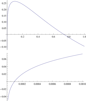
Figure 1: $\left(\frac{G_{11}}{g_{11}}/G_{00}\right)$ versus $\gamma=\frac{t}{t_{0}}$ graph for $\beta=50$, $\xi=1$

The general form of the cosmic history must have a cosmic acceleration era corresponding to the time of inflation that is followed by an era of deceleration at the matter dominated era, and finally by the present time acceleration era. Moreover the redshift values and ages for these eras must coincide with the observational data PDG at least at the order of magnitude to have at least an approximately realistic model. For this purpose we draw $\frac{\ddot{a}}{a}/G_{00}$ versus time for $\xi$=0.8,, 1, 1.2; $\beta$=2, 5, 10, 20, 50, 100, 200, 500, 1000, 2000, 10000, 3000, 40000 by using

$$\frac{\frac{\ddot{a}}{a}}{G_{00}} = -\frac{(a_{2})^{\frac{1}{6}}b_{1}(p_{1}+p_{2}a_{2}t)[\frac{b_{1}}{(a_{2}t)^{\frac{1}{6}}}(p_{1}+p_{2}a_{2}t)+(-7p_{1}+5p_{2}a_{2}t)]}{3(a_{2}t)^{\frac{1}{3}}[6p_{2}a_{2}t+\frac{b_{1}}{(a_{2}t)^{\frac{1}{6}}}(p_{1}+p_{2}a_{2}t)]}$$

$$= -\left(\frac{ln{\beta}}{3\gamma^{\frac{1}{6}}}\right)\frac{A[(\gamma^{-\frac{1}{6}}\ln{\beta})A-7(1-\xi+\frac{1}{6}\ln{\beta})+5\gamma\xi-\frac{5}{6}\gamma\ln{\beta}]}{6(\xi-\frac{1}{6}\ln{\beta})\gamma+\gamma^{-\frac{1}{6}}\ln{\beta}[1-(1-\gamma)\xi+\frac{1-\gamma}{6}\ln{\beta}]}$$

$$A\,=\,[1-(1-\gamma)\xi+\frac{(1-\gamma)}{6}\ln{\beta}]$$

where $\gamma=\frac{t}{t_{0}}$. One may get a sense of the general form of the evolution in Figure 2 for $\beta=50$, $\xi=1$.

Figure 2: $\frac{\ddot{a}}{a}/G_{00}$ versus $\gamma=\frac{t}{t_{0}}$ graph for $\beta=50$, $\xi=1$

I do not give the other plots not to make the paper too crowded. The all values of the times of the start and the end of cosmic deceleration that are not wholly excluded by data are given in Table 2 below. It seems that this analysis prefers lower values of $\beta$. Note that we should not expect a good match between the values obtained here and the observational data for the time of the start of the deceleration period because at that time the radiation has a major contribution and we neglect the contribution of radiation in this study.

$\xi$	$\beta$	$\gamma_{mi}$	$\gamma_{mf}$	$\xi$	$\beta$	$\gamma_{mi}$	$\gamma_{mf}$
0.8	2	$10^{-6}$	0.5	0.8	5	$1.5\times 10^{-4}$	0.7
0.8	10	$1.2\times 10^{-3}$	0.9	0.8	200	0.165	0.947
0.8	500	0.28	0.89	0.8	1000	0.35	0.867
0.8	2000	0.58	0.91	-	-	-	-
1	2	$9.5\times 10^{-7}$	0.13	1	5	$1.4\times 10^{-4}$	0.26
1	10	$1.3\times 10^{-3}$	0.34	1	20	$6.6\times 10^{-3}$	0.415
1	50	0.04	0.45	1	100	0.116	0.7
1	1000	0.48	0.945	1	2000	0.52	0.916

Table 2: The times of start, $\frac{t_{mi}}{t_{0}}$ and end, $\frac{t_{mf}}{t_{0}}$ of the cosmic deceleration for different values of $\beta$

Now we compare the data and the predictions of this model for different redshifts and times, and hope, at least, an order of magnitude agreement. First consider the time of the starting of cosmic acceleration. This is the time where the deceleration changes into acceleration, hence the acceleration of the cosmic expansion is zero i.e. the numerator of (5) is zero, namely

$$f\,=\,\frac{1-\gamma_{d}}{6}x^{2}+[1-(1-\gamma_{d})\xi-\frac{7}{6}\gamma_{d}^{\frac{1}{6}}-\frac{5}{6}\gamma_{d}^{\frac{7}{6}}]x-7(1-\xi)\gamma_{d}^{\frac{1}{6}}\,=\,0$$ (41)

$$~{}~{}\gamma_{d}\,=\,\frac{t_{d}}{t_{0}}~{}~{}~{},~{}~{}~{}x\,=\,\ln{\beta}$$

Because of its highly non-linear form this equation I could not analytically solve this equation. However after plotting $f$ versus x for various values of $\xi$ and $\gamma_{d}$ and determining the location of zeros one may get some information. The result is given in Table 3.

$\xi$	$\gamma_{d}$	$x=\ln{\beta}$	$\xi$	$\gamma_{d}$	$x=\ln{\beta}$
0.8	0.85	2 or 26	0.8	0.8	2 or 25
0.8	0.75	2 or 20	0.8	0.7	2 or 16
0.8	0.5	0.7 or 9	0.8	0.4	0.2 or 7.8
0.8	0.1	1 or 5	0.8	$10^{-10}$	-1.2 or 0.2
0.8	$10^{-20}$	-1.2 or 0	1	0.85	5 or 35
1	0.8	5 or 24	1	0.75	5 or 17
1	0.7	5 or 15	1	0.5	3.6 or 7.2
1	0.3	1.9 or 5.5	1	0.1	0.5 or 4.5
1	$10^{-10}$	0.06 or 0.09	1	$10^{-20}$	0 or 0.0033
1.2	0.85	7 or 33	1.2	0.8	7 or 22
1.2	0.75	8.7 or 15.7	1.2	0.5	none

Table 3: The allowed values of $ln{\beta}$ for various values of $\xi$ and $\gamma_{d}$

Keeping these values in mind now we may find the redshift values and the time of onset of current cosmic acceleration, $t_{d}$ predicted by this model and compare the observational values given in literature. Consider $a_{0}/a(t_{d})$

$$\frac{a_{0}}{a(t_{d})}\,=\,\frac{\exp{[b_{1}(a_{2}t_{d})^{-\frac{1}{6}}]}}{(p_{1}+p_{2}a_{2}t_{d})}\,=\,\frac{\beta^{-1+\gamma_{d}^{-\frac{1}{6}}}}{(1-\xi)+\frac{1}{6}\ln{\beta}+(\xi-\frac{1}{6}\ln{\beta})\gamma_{d}}$$ (43)

The analysis of cosmic data onset gives the redshift and time of onset of dark energy dominated era, respectively, in the ranges $z\,=\,0.66\,-\,1.21$. $t_{d}\,=\,(5.7\,-\,8.5)\,Gyr$. The allowed intervals of $\beta$ in (43) where $\frac{a_{0}}{a(t_{d})}$ is in the range $\,1.66\,--\,2.21$ for the phenomenologically relevant values of $\xi$ and $\gamma_{d}=\frac{t_{d}}{t_{0}}$ for $\xi$= 0.8, 1, 1.2 and $\gamma_{d}$=0.1, 0.4, 0.5, 0.6, 0.7, 0.8 may be found in Table 4.

$\xi$	$\gamma_{d}$	$\beta$
0.8	0.1	none
0.8	0.4	0.15 — 123
0.8	0.5	1 — $7\times 10^{3}$
0.8	0.6	$2\times 10^{3}~{}---~{}2.1\times 10^{6}$ and $1.8\times 10^{-3}~{}---~{}2.5\times 10^{-2}$
0.8	0.8	$5\times\,10^{12}~{}---~{}2.5\times\,10^{18}$ and $7\times\,10^{-9}~{}---~{}3\times\,10^{-7}$
1	0.1	none
1	0.4	none
1	0.5	4 — 1400
1	0.6	$130~{}---~{}7\times 10^{5}$ and $1.2\times\,10^{-2}~{}---~{}1$
1	0.7	$7.5\times 10^{5}~{}---~{}10^{10}$ and $1.7\times\,10^{-4}~{}---~{}5\times\,10^{-3}$
1	0.8	$1.5\times\,10^{12}~{}---~{}\,10^{18}~{}~{}\mbox{and}~{}~{}~{}5\times\,10^{-8}~{}---~{}2.8\times\,10^{-6}$
1.2	0.1	none
1.2	0.4	none
1.2	0.5	barely 30
1.2	0.6	$0.5~{}---~{}2\times\,10^{5}$
1.2	0.7	$9\times 10^{4}~{}---~{}3.5\times\,10^{9}$ and $10^{-3}~{}---~{}9\times\,10^{-2}$
1.2	0.8	$10^{12}~{}---~{}5\times\,10^{17}$ and $2.6\times\,10^{-7}~{}---~{}2.1\times\,10^{-5}$

Table 4: The allowed range of values of $\beta$ for various values of $\xi$, $\gamma$ with $\frac{a_{0}}{a(t_{d})}$ in the range $\,1.66\,--\,2.21$

Table

-atd-b

tells us that $\gamma_{d}=0.1$ is inconsistent with data. Comparison with Eq.(38) and Table 1 implies that the $\gamma_{d}$ values in the range 0.4 - 0.6 are consistent with redshift data onset and the time of the onset of the cosmic acceleration for the phenomenologically relevant values of $\xi$ in the range 1.2 - 0.8. An important point is to be mentioned at this point: Note that the values $z\,=\,0.66\,-\,1.21$, $t_{d}\,=\,(5.7\,-\,8.5)\,Gyr$ in onset1 are derived by the assumption that the Hubble constant at scale factor $a(t)$ may be expressed as

$$H(a)\,=\,H_{0}\,[\frac{\Omega_{m}}{a^{3}}+\frac{\Omega_{r}}{a^{4}}+\frac{\Omega_{k}}{a^{2}}+\frac{\Omega_{\Lambda}}{a^{3(1+\omega_{eff}(a))}}\,]^{\frac{1}{2}}$$ (44)

In principle one may define an effective equation of state $\omega_{eff}$ as in Sola2 when dark matter and dark energy are coupled. However in this model the contributions of dark matter and dark energy are not only coupled they are mixed. Therefore their contributions can not be separated from each other properly. Moreover dark matter in this model is not dust-like (it only mimics a dust in the matter dominated era) while the matter in the above equation is dust-like. Furthermore in onset1 and similar studies an equation of state for dark energy of the form $\omega(a)\,=\,-\omega_{0}+\omega_{1}(1-a)$ or similar forms are employed. Let alone that a proper equation of state for dark energy in this model can not be defined a common equation of state for dark energy and dark matter is highly nonlinear as seen before in Eq.(39)

$$\frac{\frac{G_{11}}{g_{11}}}{G_{00}} = -\frac{\frac{\ln{\beta}}{12\gamma^{\frac{7}{3}}}+\frac{(\xi-\frac{1}{6}\ln{\beta})^{2}}{[1-(1-\gamma)\xi+\frac{(1-\gamma)}{6}\ln{\beta}]^{2}}+\frac{11((\xi-\frac{1}{6}\ln{\beta})^{2}\ln{\beta}}{18\gamma^{\frac{7}{6}}(1-(1-\xi)\gamma+\frac{(1-\gamma)}{6}\ln{\beta})}-\frac{7(1-\xi+\frac{1}{6}\ln{\beta})\ln{\beta}}{18\gamma^{\frac{13}{6}}(1-(1-\xi)\gamma+\frac{(1-\gamma)}{6}\ln{\beta})}}{3\left(\gamma^{-\frac{7}{6}}\frac{\ln{\beta}}{6}+\frac{\xi-\frac{1}{6}\ln{\beta}}{(1-(1-\xi)\gamma+\frac{(1-\gamma)}{6}\ln{\beta})}\right)^{2}}$$ (45)

An inspection of $[a(t)]^{-1}$ versus $\gamma_{0}=\frac{t}{t_{0}}$ graphs show that in the low redshift range z= 05 - 2 one may approximately take $[a(t)]^{-1}$ proportional to $\gamma$. In other words one may get the form of $\omega(a)$ for low redshifts by simply replacing $\gamma$ in (45) by 1+z. It is evident that this relation is quite nonlinear in z. For higher redshift values the relation between $\gamma$ and (z+1)^-1 also becomes non-linear making the form of $\omega(a)$ even more complicated. Therefore in order to see the degree of the compatibility of this model with data in a more precise way it is necessary to repeat the analysis of data in onset ; onset1 with keeping these points in mind. Only then one can say some definite conclusion on the degree of the agreement between this model and observational data. In any case I think the rough analysis given in this paper is enough to consider this model as viable toy model in the direction of unification of all eras of cosmic history. In fact all I have mentioned in the context of the analysis of the onset of cosmic acceleration data is true for the analysis of data for equation of state of dark energy Amanullah , density parameters wider-omega , and the analysis of data on time reionization and time of matter-radiation decoupling PDG ; Komatsu discussed below. Before continuing the comparison of the model with observational analysis for the times of reionization and decoupling now I want to consider the inflationary era because there is no baryonic matter or radiation effect in this era, this toy model is expected to be most similar to the reality in this era in the context of this model. It is evident from (5) that, at the time of inflation,

$$b_{1}(p_{1}+p_{2}a_{2}t)+(a_{2}t)^{\frac{1}{6}}(-7p_{1}+5p_{2}a_{2}t)\,>\,0$$ (46)

This condition is satisfied for very large and very small $a_{2}t$’s. We identify the very small $a_{2}t$ values that satisfy (46) as inflationary times, and at small times (46) is guaranteed if we take $a_{2}t_{i}\,\ll\,1$ where the subindex $i$ refers to inflation. In fact a more stringent bound may be obtained from the slow-roll parameter $\frac{\dot{H}}{H^{2}}$ in (4)

$$\frac{\dot{H}(t_{i})}{H^{2}(t_{i})}\,\simeq\,-\frac{7\gamma_{i}^{\frac{1}{6}}}{\ln{\beta}}\,\ll\,1~{}~{}~{}\Rightarrow~{}~{}~{}~{}\gamma_{i}=\frac{t_{i}}{t_{0}}\,\ll\,1$$ (47)

where we have used the fact that the $p_{1}$ term in (4) is the leading term in the inflationary period. Then

$$\frac{a(t_{is})}{a(t_{il})} = \frac{(p_{1}+p_{2}a_{2}t_{is})\exp{\{-b_{1}[(a_{2}t_{is})^{-\frac{1}{6}}-(a_{2}t_{il})^{-\frac{1}{6}}]\}}}{(p_{1}+p_{2}a_{2}t_{il}}$$

$$= \left(\frac{1-(1-\gamma_{is})\xi+\frac{(1-\gamma_{is})}{6}\ln{\beta}}{1-(1-\gamma_{il})\xi+\frac{(1-\gamma_{il})}{6}\ln{\beta}}\right)\exp{\{-\frac{b_{1}}{a_{2}^{\frac{1}{6}}}[t_{is}^{-\frac{1}{6}}-t_{il}^{-\frac{1}{6}}]\}}\,\simeq\,\exp{\{-\frac{b_{1}}{a_{2}^{\frac{1}{6}}}[t_{is}^{-\frac{1}{6}}-t_{il}^{-\frac{1}{6}}]\}}$$

where $t_{is}$ and $t_{il}$ are the times of the start and end of inflation, respectively. If we assume 60 e-fold expansion and $t_{is}=\,=\,10^{-36}\,sec$, $t_{il}\,=\,10^{-32}\,sec$

$$\frac{a(t_{is})}{a(t_{il})} \simeq \exp{[-b_{1}\,(a_{2})^{-\frac{1}{6}}10^{6}(sec)^{-\frac{1}{6}}]}\,=\,e^{60}$$ (49)

$$\Rightarrow~{}~{}~{}~{}~{}b_{1}a_{2}^{-\frac{1}{6}}\times\,10^{6}\,sec^{-\frac{1}{6}}\,=\,60$$

$$\Rightarrow\,~{}~{}~{}~{}b_{1}a_{2}^{-\frac{1}{6}}\,\simeq\,6\times\,10^{-5}\,sec^{\frac{1}{6}}~{}~{}~{}~{}\Rightarrow\,~{}~{}~{}~{}\ln{\beta}\,=\,8.8\times\,10^{-8}$$

If we assume 60 e-fold expansion and $t_{is}=\,=\,10^{-28}\,sec$, $t_{il}\,=\,t_{is}+10^{-34}\,sec$

$$\frac{a(t_{is})}{a(t_{il})} \simeq \exp{\{-b_{1}\,(a_{2})^{-\frac{1}{6}}(1\times\,10^{-30})^{-\frac{1}{6}}[(100)^{-\frac{1}{6}}\,-\,(100.0001)^{-\frac{1}{6}}]\}}\,=\,e^{60}$$ (50)

$$\Rightarrow~{}~{}~{}~{}~{}b_{1}a_{2}^{-\frac{1}{6}}\times\,7.7\times\,10^{-3}\,=\,60$$

$$\Rightarrow\,~{}~{}~{}~{}b_{1}a_{2}^{-\frac{1}{6}}\,\simeq\,7.8\,\times\,10^{3}~{}~{}~{}~{}\Rightarrow\,~{}~{}~{}~{}\ln{\beta}\,=\,11$$

Note that

$$b_{1}a_{2}^{-\frac{1}{6}}\,=\,b_{1}(a_{2}t_{0})^{-\frac{1}{6}}t_{0}^{\frac{1}{6}}\,=\,t_{0}^{\frac{1}{6}}\,\ln{\beta}$$ (51)

Some other values of $t_{is}$, $t_{il}$ and $\ln{\beta}$ for 60 e-fold expansion are

$$t_{is}\,=\,10^{-30}\,sec~{}~{}~{}~{}~{}~{}t_{il}\,=\,t_{is}+10^{-34}~{}~{}~{}~{}\Rightarrow~{}~{}~{}~{}\ln{\beta}\,=\,5.57\times\,10^{-2}$$ (52)

$$t_{is}\,=\,10^{-24}\,sec~{}~{}~{}~{}~{}~{}t_{il}\,=\,t_{is}+10^{-34}\,sec~{}~{}~{}~{}\Rightarrow~{}~{}~{}~{}\ln{\beta}\,=\,5.57\times\,10^{5}$$ (53)

$$t_{is}\,=\,10^{-28}\,sec\,+\,10^{-34}\,sec~{}~{}~{}~{}~{}~{}t_{il}\,=\,t_{is}+2\times\,10^{-34}\,sec~{}~{}~{}~{}\Rightarrow~{}~{}~{}~{}\ln{\beta}\,=\,5.72$$ (54)

$$t_{is}\,=\,10^{-28}\,sec\,+\,10^{-34}\,sec~{}~{}~{}~{}~{}~{}t_{il}\,=\,t_{is}+2.4\times\,10^{-34}\,sec~{}~{}~{}~{}\Rightarrow~{}~{}~{}~{}\ln{\beta}\,=\,8.15$$ (55)

$$t_{is}\,=\,10^{-29}\,sec\,~{}~{}~{}~{}~{}~{}t_{il}\,=\,t_{is}+5\times\,10^{-34}\,sec~{}~{}~{}~{}\Rightarrow~{}~{}~{}~{}\ln{\beta}\,=\,0.13$$ (56)

One notices that (49), (52), (54), (56) are consistent with (32) while the others are not. However it seems that the values in Table I exclude the values of $\ln{\beta}$ much smaller than 1. This excludes the options in (49) and (52) as well. Hence the viable values seem to be (54) and (56) and all values of parameters between them and close to these values. This offers a wide range of $t_{is}$ between $10^{-28}\,sec$ and $10^{-29}\,sec$. It is evident that all phenomenologically viable values may be obtained by adjusting $t_{is}$ in the $t_{is}=10^{-29}\,sec$ – $t_{is}=10^{-28}\,sec$ range that corresponds to a lower scale inflation lower . A comment is in order at this point. From Eq.(5) we see that just at the end of the inflationary era

$$b_{1}(p_{1}+p_{2}a_{2}t_{mi})+(a_{2}t_{mi})^{\frac{1}{6}}(-7p_{1}+5p_{2}a_{2}t_{mi})\,\leq\,0$$ (57)

$$\Rightarrow~{}~{}~{}~{}p_{1}\frac{b_{1}}{(a_{2}t_{mi})^{\frac{1}{6}}}-7p_{1}+\epsilon=0$$ (58)

$$\left(\gamma_{mi}^{-\frac{1}{6}}\ln{\beta}-7\right)(1-\xi+\frac{1}{6}\ln{\beta})+\epsilon^{\prime}\,=\,0$$ (59)

$$~{}~{}~{}~{}\epsilon=\frac{b_{1}}{(a_{2}t)^{\frac{1}{6}}}p_{2}a_{2}t+5p_{2}a_{2}t~{},~{}~{}\epsilon^{\prime}=\frac{\epsilon}{\beta}=\gamma_{mi}(\gamma_{mi}^{-\frac{1}{6}}\ln{\beta}+5)(\xi-\frac{1}{6}\ln{\beta})$$

where the first two terms in (58) are the dominant terms and $\epsilon$ (and $\epsilon^{\prime}$) is small with respect to the others. The fact that $\epsilon^{\prime}$ in and at the end of inflationary era is small implies that either $(\gamma_{mi}^{-\frac{1}{6}}\ln{\beta}-7)$ or $(1-\xi+\frac{1}{6}\ln{\beta})$ is small. Taking $t_{mi}\sim\,t_{il}\sim\,10^{-28}--10^{-29}$ i.e. $\gamma_{mi}=\frac{t_{mi}}{t_{0}}\sim\,10^{-46}$ implies that $(\gamma_{mi}^{-\frac{1}{6}}\ln{\beta}-7)$ is not small unless $\ln{\beta}$ is extremely small. Therefore $(1-\xi+\frac{1}{6}\ln{\beta})$ should be small if deceleration era starts just after the inflationary era. This may be provided by taking $\xi$ a little bit larger than 1 and $\ln{\beta}$ small. For example one may take $\xi=1.05$ and $\ln{\beta}\sim\,0.3$ (i.e. $\beta\sim\,1.35$). Otherwise one should take the start of the deceleration era much later than the standard inflationary era (i.e. the inflationary era is much longer than the standard inflationary times). Although this option seems to be a less acceptable option it is, in fact, the more reasonable choice. This is due to the fact that we neglect radiation in this study. In the realistic case there is a radiation dominated era just after the inflationary era. Radiation like matter drives the universe towards deceleration. Therefore if we add radiation to the model it is effect will be an earlier start of deceleration era compared to the radiationless case. This explains why the time of the start of the deceleration period almost coincides with the time of start of the matter dominated era in Table (2) unless $\beta$ is extremely close to 1. In other words the values of parameters become less reliable as we get closer to the radiation dominated era. We should keep this in mind as we analyze the observational data. Now we apply the values obtained to the time of reionization, $t_{ri}$. In fact we expect, at most, a rough agreement with data since $t_{ri}$ goes deeper into the matter dominated era where neglecting baryonic matter becomes more questionable.

$$\frac{a_{0}}{a(t_{ri})}\,=\,\frac{\exp{[b_{1}(a_{2}t_{ri})^{-\frac{1}{6}}]}}{(p_{1}+p_{2}a_{2}t_{ri})}\,=\,\frac{\beta^{\gamma_{ri}^{-\frac{1}{6}}}}{(1-\xi)\beta+\frac{1}{6}\ln{\beta}+(\xi\beta-\frac{1}{6}\ln{\beta})\gamma_{ri}}$$ (60)

where $\gamma_{ri}=\frac{t_{ri}}{t_{0}}$. The observational value of $\frac{a_{0}}{a(t_{ri})}$ is $12\pm\,1.4$ and the corresponding $\Lambda$CDM value of $t_{ri}$ is 430${}^{+90}_{-70}$ Myr that corresponds to $\gamma_{ri}$ in the interval $0.0225~{}---~{}0.0472$ if one assumes a loose bound on the value of $t_{0}$, $t_{0}\,=\,11~{}---~{}16\;Gyrs$ in the light of the values of $t_{0}$ from different observations mentioned before. One may plot $\frac{a_{0}}{a(t_{ri})}$ versus $\gamma=\frac{t}{t_{0}}$ for the phenomenologically relevant values of $\xi$ and various $\beta$ values. The allowed intervals of $\gamma_{d}$ for $\frac{a_{0}}{a(t_{ri})}$ in the interval 10.6 - 12.4 for various values of $\xi$ and $\beta$ may be found in Table 5.

$\xi$	$\beta$	$\gamma_{ri}$	$\xi$	$\beta$	$\gamma_{ri}$
0.8	2	0.0016 — 0.0023	0.8	5	0.0115 — 0.016
0.8	10	0.023 — 0.03	0.8	20	0.037  — 0.046
0.8	50	0.058 — 0.068	0.8	100	0.074 — 0.086
0.8	200	0.091 — 0.105	0.8	500	0.116 — 0.128
0.8	1000	0.13 — 0.146	0.8	2000	0.15 — 0.162
1	2	0.028 — 0.041	1	5	0.029 — 0.041
1	10	0.04 — 0.051	1	20	0.054  — 0.066
1	50	0.079 — 0.086	1	100	0.089 — 0.104
1	200	0.105 — 0.12	1	500	0.13 — 0.142
1	1000	0.142 — 0.16	1	2000	0.16 — 0.18
1.2	2	0.17 — 0.19	1.2	5	0.105 — 0.125
1.2	10	0.09 — 0.105	1.2	20	0.091  — 0.104
1.2	50	0.098 — 0.116	1.2	100	0.114 — 0.127
1.2	200	0.125 — 0.142	1.2	500	0.144 — 0.162
1.2	1000	0.159 — 0.177	1.2	2000	0.173 — 0.192

Table 5: The allowed range of values of $\gamma_{ri}=\frac{t_{ri}}{t_{0}}$ for various values of $\xi$, $\gamma$ with $\frac{a_{0}}{a(t_{d})}$ in the range $\,10.6\,--\,12.4$

It seems that the values of $\beta$ compatible with data are 10, 20 for $\xi$= 0.8; 2, 5, 10 for $\xi$= 1; and none for $\xi$=1.2. However one should keep in mind that a more detailed analysis may give a wider range of parameters since the age calculations in the data analysis Komatsu2009 use a restricted form for dark energy where Hubble constant may be expressed in terms of density parameters where matter is assumed dust-like and a restricted form of variation of dark energy with redshift, and a restricted class of equations of state for dark energy where dark energy is not entangled with matter as pointed out before. Therefore reanalysis of data in the context of this model is necessary to reach a more precise and more definite conclusion. Another factor for poorer agreement with data is that we neglect the contribution of baryonic matter whose contribution in matter dominated period is greater. Next consider the data for the time of decoupling and the corresponding redshift; $z_{*}\,\simeq\,1090$

$$\frac{a_{0}}{a(t_{*})}\,=\,\frac{\exp{[b_{1}(a_{2}t_{*})^{-\frac{1}{6}}]}}{(p_{1}+p_{2}a_{2}t_{*})}\,=\,\frac{\beta^{\gamma_{*}^{-\frac{1}{6}}}}{(1-\xi)\beta+\frac{1}{6}\ln{\beta}+(\xi\beta-\frac{1}{6}\ln{\beta})\gamma_{*}}$$ (61)

where $\gamma_{*}=\frac{t_{*}}{t_{0}}$. One may plot $\frac{a_{0}}{a(t_{*})}$ versus $\gamma=\frac{t}{t_{0}}$ for various values of $\xi$ and $\beta$. The values of $\gamma_{*}$ corresponding to the observational value of $\frac{a_{0}}{a(t_{*})}\sim\,1090$ are given in Table 6.

$\xi$	$\beta$	$\gamma_{ri}$	$\xi$	$\beta$	$\gamma_{ri}$
0.8	2	$1.42\times\,10^{-6}$	0.8	5	$7.45\times\,10^{-5}$
0.8	10	$3.3\times\,10^{-4}$	0.8	20	$9.05\times\,10^{-4}$
0.8	50	$2.32\times\,10^{-3}$	0.8	100	$3.99\times\,10^{-3}$
0.8	200	$6.17\times\,10^{-3}$	0.8	500	$9.86\times\,10^{-3}$
0.8	1000	$1.32\times\,10^{-2}$	0.8	2000	$1.71\times\,10^{-2}$
1	2	$3.9\times\,10^{-6}$	1	5	$1.15\times\,10^{-4}$
1	10	$4.44\times\,10^{-4}$	1	20	$1.12\times\,10^{-3}$
1	50	$2.7\times\,10^{-3}$	1	100	$4.5\times\,10^{-3}$
1	200	$6.8\times\,10^{-3}$	1	500	$1.06\times\,10^{-2}$
1	1000	$1.425\times\,10^{-2}$	1	2000	$1.81\times\,10^{-2}$
1.2	2	$7.91\times\,10^{-2}$	1.2	5	$7.45\times\,10^{-5}$
1.2	10	$3.3\times\,10^{-4}$	1.2	20	$1.56\times\,10^{-3}$
1.2	50	$3.34\times\,10^{-3}$	1.2	100	$5.28\times\,10^{-3}$
1.2	200	$7.7\times\,10^{-3}$	1.2	500	$1.17\times\,10^{-2}$
1.2	1000	$1.53\times\,10^{-2}$	1.2	2000	$1.95\times\,10^{-2}$

Table 6: The allowed range of values of $\gamma_{*}=\frac{t_{*}}{t_{0}}$ for various values of $\xi$, $\gamma$ with $\frac{a_{0}}{a(t_{d})}\,\sim\,1090$

Inspection of the table suggests there are no of the values are $\xi$ and $\beta$ compatible with observational value $t_{*}\,\simeq\,3.8\times 10^{5}\,yr$ Komatsu2009 that corresponds to the interval $\gamma_{*}=\frac{t_{*}}{t_{0}}\,=\,2.375\times 10^{-5}~{}---~{}3.4545\times 10^{-5}$ (provided that $t_{0}\,=\,(11~{}---~{}16)\,Gyrs$) except for $\xi=0.8,\,1$ and $\beta$ somewhere between 2 and 5 (i.e. $\sim$ 3.7, 3) while the values for $\xi=0.8$, $\beta=5$ and $\xi=1.2$, $\beta=5$ are close to the relevant values. In fact this poor agreement with those given in Komatsu2009 is expected. In addition to the reasons mentioned for the reionization time there is an important additional source of discrepancy. The time of matter radiation decoupling time is quite close to the radiation dominated era. The ratio of radiation in this period in the order of a fourth of the total energy density at this time while this model neglects the contribution of radiation. To summarize the results of this section can be stated as follows: We have seen that the predictions of this model for each of $\left(\frac{\ddot{a}}{a}/G_{00}\right)_{t=t_{0}}$, $\left(\frac{G_{11}}{g_{11}}/G_{00}\right)_{t=t_{0}}$, $a_{0}/a(t_{d})$, $a_{0}/a(t_{ri})$ are compatible with observations although not with central values given in literature. The prediction of the model for $a_{0}/a(t_{*})$ is partially consistent with observational values. In fact the relatively less compatibility for the decoupling time $t_{*}$ is expected since the radiation-matter decoupling time is close to the radiation dominated era while radiation is ignored in this study. I have also shown that an inflationary era naturally fits the model. One may consider the simultaneous compatibility of the predictions of all these parameters with observations as well. In all cases there is wide range of $\beta$’s compatible with Eq.(32). The values of $\beta$ allowed by (38) includes the values allowed by Table 1, that is, Table 1 and (38) are compatible while Table 1 is more restrictive. The values of $\gamma_{d}$ in Table 3 that are compatible with Table 4 are $\xi$=0.8 $\Rightarrow$ $\gamma_{d}$=0.4 or $\gamma_{d}$=0.5, $\xi$=1 $\Rightarrow$ $\gamma_{d}$=0.5 or $\gamma_{d}$=0.8, $\xi$=1.2 $\Rightarrow$ hardly $\gamma_{d}$=0.8. The values of $\xi$, $\gamma_{d}$ in Table 4 whose $\beta$ values compatible with the $\beta$ values in Table 1 are $\xi$=0.8, $\gamma_{d}$=0.4, $\gamma_{d}$=0.5, $\beta$= 2.14 – 12.2; $\xi$=1, $\gamma_{d}$=0.5 $\Rightarrow$ $\beta$= 4 – 144; $\xi$=1, $\gamma_{d}$=0.6 $\Rightarrow$ $\beta$= 130 – 147; $\xi$=1.2, $\gamma_{d}$=0.6 $\Rightarrow$ Table 1 and Table 4 are compatible except for lowest values of $\beta$. Mostly Table 1 is more restrictive than Table 4. The values of $\gamma_{ri}$ in Table 5 that are more compatible with observational value $\gamma_{ri}$= 0.0225 – 0.0472 in literature Komatsu2009 seem to prefer $\beta$ in the range 2 – 10. I do not use Table 6 to constraint $\beta$ since the time of decoupling is close to the radiation dominated era while we do ignore radiation, so the reliability of the values obtained is questionable, and an order of magnitude compatibility is enough. We see that compatibility of the values of all these tables seem to prefer values $\xi$ = 0.8 - 1, $\beta$ = 2 - 10. However these values of $\beta$ are at the edge of the observationally allowed values rather than being centrally allowed values. The limited overall compatibility of the results of this model with observations may either be due to this model being simply a toy model or the inapplicability of some of the assumptions of the analysis in literature to this model such as Eq.(44) and $\omega(a)\,=\,-\omega_{0}+\omega_{1}(1-a)$ or a combination of both. In fact, even a standard analysis may be enough to check the viability of this model beyond a toy model for small enough redshift bins. For example, it seems that the allowed value of the equation of state for dark energy, $\omega_{DE}$ at the smallest redshift bin in Figure 14 of Amanullah may be as large as -1/3 while the $G_{11}/G_{00}$ versus $\beta$ graph for this model at present time (for $\xi=1$) gives $G_{11}/G_{00}\simeq\,-0.45$ (that corresponds to $\omega_{DE}\sim\,-0.65$ for $\Omega_{DE}=0.74$) for $\beta\sim\,3$. A definite conclusion needs a detailed comprehensive reanalysis of all data in the light of this model in a separate study.

IV conclusion

I have considered a model where inflationary era and (dark) matter dominated eras are induced by a scalar field $\phi_{1}$ while the dark energy dominated era is induced by another scalar $\phi_{2}$. These fields may be either considered to be fundamental fields or as effective classical fields. I prefer to consider them as classical fields rather than true fundamental fields. I have neglected the effects of baryonic matter and radiation. A rough phenomenological analysis of cosmic data gives an order of magnitude agreement with data. This is encouraging for future studies in this direction. One must include baryonic matter and radiation to obtain a more realistic model. However this is not an easy task. First difficulty is that baryonic matter and radiation should be included after the time of inflation because it should be produced by the decay of one of the scalars (probably by $\phi_{1}$). Second, even when one includes them in ad hoc way this modifies the metric. Hence one must find the scale factor that corresponds to inclusion of the baryonic matter and radiation and this not a trivial task. Another point that needs further study is a more detailed and comprehensive analysis of the available parameter space and to find the most optimal set. Yet another point for further study is the study of cosmological perturbations produced in the inflationary epoch. The inflation obtained here is a standard slow-roll inflation with the canonical kinetic terms for the scalars. Therefore the general form of the perturbations is the same as the usual slow-roll case Weinberg . However a detailed study of the perturbations in this model should be obtained to compare with the expectations of the other models for data to be obtained in future cosmological observations. All these points need further separate studies.