Submillimeter continuum observations of Sagittarius B2 at subarcsecond spatial resolution

We report the first high spatial resolution submillimeter continuum observations of the Sagittarius B2 cloud complex using the Submillimeter Array (SMA). With the subarcsecond resolution provided by the SMA, the two massive star-forming clumps Sgr B2(N) and Sgr B2(M) are resolved into multiple compact sources. In total, twelve submillimeter cores are identified in the Sgr B2(M) region, while only two components are observed in the Sgr B2(N) clump. The gas mass and column density are estimated from the dust continuum emission. We find that most of the cores have gas masses in excess of 100 M_⊙ and column densities above 10²⁵ cm^-2. The very fragmented appearance of Sgr B2(M), in contrast to the monolithic structure of Sgr B2 (N), suggests that the former is more evolved. The density profile of the Sgr B2(N)-SMA1 core is well fitted by a Plummer density distribution. This would lead one to believe that in the evolutionary sequence of the Sgr B2 cloud complex, a massive star forms first in an homogeneous core, and the rest of the cluster forms subsequently in the then fragmenting structure.

1 Introduction

The Sagittarius B2 star-forming region is located $\sim$ 100 pc from Sgr A^∗, within the $\sim 400$ pc wide dense central molecular zone (CMZ) of the Galactic center, at a distance of $\sim$8 kpc from the Sun (Reid et al. 2009). It is the strongest submillimeter continuum source in the CMZ (Schuller et al. 2009). It contains dense cores, Sgr B2(N) and Sgr B2(M), hosting clusters of compact Hii regions (Gaume et al. 1995; de Pree, Goss & Gaume 1998). It has been suggested that these two hot cores are at different evolutionary stages (Reid et al 2009; Lis et al. 1993; Hollis et al. 2003; Qin et al. 2008). Spectral observations in centimeter and millimeter regimes have been conducted towards Sgr B2 (e.g. Carlstrom & Vogel 1989; Mehringer & Menten 1997; Nummelin et al. 1998; Liu & Snyder 1999; Hollis et al. 2003; Friedel et al. 2004; Jones et al. 2008; Belloche et al. 2008), suggesting that Sgr B2(N) is chemically more active. Nearly half of all known interstellar molecules were first identified in Sgr B2(N), although sulphur-bearing molecules are more abundant in Sgr B2(M) than in Sgr B2(N).

The differences between Sgr B2(N) and Sgr B2(M), in terms of both kinematics and chemistry, may originate from different physical conditions and thus different chemical histories, or may simply be an evolutionary effect. A clearer understanding of the small-scale source structure and the exact origin of the molecular line emission is needed to distinguish between these two possibilities. In this Letter, we present high spatial resolution submillimeter continuum observations of Sgr B2(N) and Sgr B2(M), using the SMA. The observations presented here resolve both of the Sgr B2 clumps into multiple submillimeter components. Combining with the SMA spectral line data cubes and ongoing Herschel/HIFI complete spectral surveys towards Sgr B2(N) and Sgr B2(M) in the HEXOS key project, these observations will help us to answer fundamental questions about the chemical composition and physical conditions in Sgr B2(N) and Sgr B2(M).

2 Observations

The SMA observations of Sgr B2 presented here were carried out using seven antennas in the compact configuration on 2010 June 11, and using eight antennas in the very extended configuration on 2010 July 11. The phase tracking centers were $\alpha\,(\mathrm{J}\,2000.0)=17^{\mathrm{h}\,}47^{\mathrm{m}\,}19.883^{\mathrm{s}\,},\delta\,(\mathrm{J}\,2000.0)=-28^{\circ}22^{\prime}18.4^{\prime\prime}$ for Sgr B2(N) and $\alpha\,(\mathrm{J}\,2000.0)=17^{\mathrm{h}\,}47^{\mathrm{m}\,}20.158^{\mathrm{s}\,},\delta\,(\mathrm{J}\,2000.0)=-28^{\circ}23^{\prime}05.0^{\prime\prime}$ for Sgr B2(M). Both tracks were observed in double-bandwidth mode with a 4 GHz bandwidth in each of the lower sideband (LSB) and upper sideband (USB). The spectral resolution was 0.8125 MHz per channel, corresponding to a velocity resolution of $\sim$0.7 km s^-1. The observations covered rest frequencies from 342.2 to 346.2 GHz (LSB), and from 354.2 to 358.2 GHz (USB). Observations of QSOs 1733-130 and 1924-292 were evenly interleaved with the array pointings toward Sgr B2(N) and Sgr B2(M) during the observations in both configurations, to perform antenna gain calibration.

For the compact configuration observations, the typical system temperature was 273 K. Mars, QSOs 3c454.3, and 3c279 were observed for bandpass calibration. The flux calibration was based on the observations of Neptune ($\sim$1.1^′′). For the very extended array observations, the typical system temperature was 292 K. Both 3c454.3 and 3c279 were used for bandpass calibration, and Uranus ($\sim$1.7^′′) was used for flux calibration. The absolute flux scale is estimated to be accurate to within 20%.

The calibration and imaging were performed in Miriad (Sault, Teuben & Wright 1995). We note that there are spectral-window-based bandpass errors in both amplitude and phase on some baselines in the compact array data, which were corrected by use of a bright point source using the BLCAL task. The system temperature measurements for antennas 2 and 7 in the very extended array data were not recorded properly and were corrected using the SMAFIX task. As done by Qin et al. (2008), we selected line free channels which may contain some contributions from weak and densely spaced blended lines, although at least obvious line contributions were excluded. The continuum images were constructed from those, combining the LSB and USB data of both the compact and very extended array observations. We performed a self-calibration on the continuum data using the model from ‘CLEANed’ components for a few iterations to remove residual errors. Using the model from ‘CLEANed’ components, the self-calibration in our case did not introduce errors in the source structure, but improved the image quality and minimized the gain calibration errors. The final images were corrected for the primary beam response. The projected baselines ranged from 9 to 80 k$\lambda$ in the compact configuration and from 27 to 590 k$\lambda$ in the very extended configuration. The resulting synthesized beam is 0$\hbox to0.0pt{.\hss}^{\prime\prime}$4$\times$0$\hbox to0.0pt{.\hss}^{\prime\prime}$24 (PA=14.4^∘) using uniform weighting, and the 1$\sigma$ rms noise levels are 21 and 31 mJy for Sgr B2(M) and Sgr B2(N) images, respectively. The difference in rms noise is caused by having more line free channels for continuum images in Sgr B2(M) (2417 channels) than in Sgr B2(N) (740 channels). Since there are no systematic offsets between the submillimeter and cm sources, we believe that the absolute astrometry is as good as 0.1^′′.

3 Results

Continuum images of Sgr B2(N) and Sgr B2(M) at 850 $\mu$m are shown in Figure 1. Multiple submillimeter continuum cores are clearly detected and resolved towards both Sgr B2(M) and Sgr B2(N) with a spatial resolution of 0$\hbox to0.0pt{.\hss}^{\prime\prime}$4$\times$0$\hbox to0.0pt{.\hss}^{\prime\prime}$24. Unlike in radio observations at 1.3 cm with a comparable resolution, which detected the UC Hii regions K1, K2, K3, and K4 (Gaume et al. 1995), only two submillimeter continuum sources, SMA1 and SMA2, are observed in Sgr B2(N) (Fig. 1). The bright component Sgr B2(N)-SMA1 is situated close to the UC Hii region K2, and Sgr B2(N)-SMA2 is located $\sim$5^′′ north of Sgr B2(N)-SMA1. The observations showed that large saturated molecules exist only within a small region ($<5^{\prime\prime}$) of Sgr B2(N) called the Large Molecule Heimat, Sgr B2(N-LMH) (Snyder, Kuan & Miao 1994). Our current observations indicate that Sgr B2(N-LMH) coincides with Sgr B2(N)-SMA1. Sgr B2(N)-SMA2 was also detected in continuum emission at 7 mm and 3 mm (Rolffs et al. 2011; Liu & Snyder 1999) and molecular lines of CH₃OH and C₂H₅CN at 7 mm (Mehringer & Menten 1997; Hollis et al. 2003). Lower resolution continuum observations at 1.3 mm (see note to Table 1 of Qin et al. 2008) suggested that the Sgr B2(N)K1-K3 clump could not be fitted with a single Gaussian component, and another component existed at Sgr B2(N)-SMA2 position. Our observations here resolved out Sgr B2(N)-SMA2, confirming it to be a high-mass core.

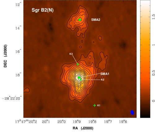
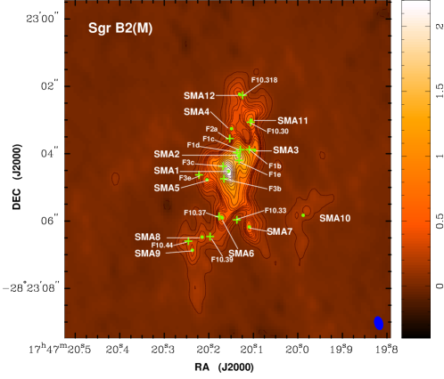
Figure 1: Continuum maps of Sgr B2 at 850 $\mu$m, with a synthesized beam of 0$\hbox to0.0pt{.\hss}^{\prime\prime}$4$\times$0$\hbox to0.0pt{.\hss}^{\prime\prime}$24, PA=14.4^∘ (lower-right corner in each panel). The left panels shows the image of Sgr B2(N), with contour levels ($-$1, 1, …14)$\times$4$\sigma$ (1$\sigma$=0.031 Jy beam^-1). The cross symbols indicate the positions of UC Hii regions detected in 1.3 cm continuum (Gaume et al. 1995). The right panel present the image of Sgr B2(M), with contour levels ($-$1, 1, 2, 3, 4, 4.5, 5.5, 5, 6, 7, 8, 10, …28)$\times$4$\sigma$ (1$\sigma$=0.021 Jy beam^-1). The cross symbols indicate the positions of UC Hii regions detected in 7 mm continuum (de Pree, Goss & Gaume 1998). In each panel, the filled circle symbols present the peak positions of the submillimeter continuum sources.

The continuum image of Sgr B2(M) (Fig. 1, right panel) shows a complicated morphology, with a roughly north-south extending envelope encompassing several compact components. In total, twelve submillimeter sources are resolved in Sgr B2(M). Using the Very Large Array (VLA), Gaume et al. (1995) detected four bright UC Hii regions (F1–F4) at 1.3 cm within 2^′′ in Sgr B2(M). The highest resolution 7 mm VLA image with a position accuracy of $0.1^{\prime\prime}$ (de Pree, Goss & Gaume 1998) resolved nineteen UC Hii regions in the central region of Sgr B2(M)(F1–F4). Five submillimeter components, Sgr B2(M)-SMA1 to SMA5, are detected in the central region of Sgr B2(M) in our observations. Outside the central region, seven components, Sgr B2(M)-SMA6 to SMA12 are identified. Given the positional accuracies of our observations and the observations by de Pree, Goss & Gaume (1998), the projected positions of Sgr B2(M)-SMA2, SMA6, SMA11 and SMA12 coincide with those of the UC HII regions F1, F10.37, F10.30, and F10.318, respectively. No centimeter source is detected towards Sgr B2(M)-SMA10, which is located south-west of the central region and displays an extended structure.

Table 1: Properties of the Continuum Sources

Source	$\alpha$ (J2000.0)	$\delta$ (J2000.0)	Deconvolved size	Peak Intensity	Flux Density	$M_{\rm H_{2}}$	$N_{\rm H_{2}}$
				(Jy beam-1)	(Jy)	(102M⊙)	($10^{25}$cm-2)
Sgr B2(N)-SMA1	17 47 19.889	–28 22 18.22	1$\hbox to0.0pt{.\hss}^{\prime\prime}72\times 1\hbox to0.0pt{.\hss}^{\prime\prime}28(-7.7^{\circ}$)	1.79$\pm$0.039	47.48$\pm$1.034	27.31$\pm$0.59	4.54$\pm$0.1
Sgr B2(N)-SMA2	17 47 19.885	–28 22 13.29	1$\hbox to0.0pt{.\hss}^{\prime\prime}44\times 1\hbox to0.0pt{.\hss}^{\prime\prime}02(-24.5^{\circ}$)	0.601$\pm$0.031	10.12$\pm$0.521	5.82$\pm$ 0.38	1.45$\pm$0.1
Sgr B2(M)-SMA1	17 47 20.157	–28 23 04.53	1$\hbox to0.0pt{.\hss}^{\prime\prime}51\times 0\hbox to0.0pt{.\hss}^{\prime\prime}59(10.6^{\circ}$)	2.39$\pm$0.138	20.9$\pm$1.21	12.02$\pm$0.7	4.94$\pm$0.29
Sgr B2(M)-SMA2	17 47 20.133	–28 23 04.06	0$\hbox to0.0pt{.\hss}^{\prime\prime}98\times 0\hbox to0.0pt{.\hss}^{\prime\prime}58(14.7^{\circ}$)	1.75$\pm$0.12	12.51$\pm$0.859	7.19$\pm$0.49	4.63$\pm$0.32
Sgr B2(M)-SMA3	17 47 20.098	–28 23 03.9	0$\hbox to0.0pt{.\hss}^{\prime\prime}93\times 0\hbox to0.0pt{.\hss}^{\prime\prime}3(-9.9^{\circ}$)	0.866$\pm$0.09	4.147$\pm$0.431	2.38$\pm$0.25	3.13$\pm$0.33
Sgr B2(M)-SMA4	17 47 20.150	–28 23 03.26	0$\hbox to0.0pt{.\hss}^{\prime\prime}55\times 0\hbox to0.0pt{.\hss}^{\prime\prime}32(-1.5^{\circ}$)	0.483$\pm$0.021	1.443$\pm$0.063	0.83$\pm$0.04	1.73$\pm$0.08
Sgr B2(M)-SMA5	17 47 20.205	–28 23 04.78	0$\hbox to0.0pt{.\hss}^{\prime\prime}66\times 0\hbox to0.0pt{.\hss}^{\prime\prime}52(15.9^{\circ}$)	0.52$\pm$0.051	2.488$\pm$0.244	1.43$\pm$0.14	1.53$\pm$0.15
Sgr B2(M)-SMA6	17 47 20.171	–28 23 05.91	0$\hbox to0.0pt{.\hss}^{\prime\prime}75\times 0\hbox to0.0pt{.\hss}^{\prime\prime}43(-24.3^{\circ}$)	0.71$\pm$0.067	3.05$\pm$0.288	1.75$\pm$0.17	1.99$\pm$0.19
Sgr B2(M)-SMA7	17 47 20.11	–28 23 06.18	0$\hbox to0.0pt{.\hss}^{\prime\prime}72\times 0\hbox to0.0pt{.\hss}^{\prime\prime}37(14.9^{\circ}$)	0.6$\pm$0.051	2.366$\pm$0.201	1.36$\pm$0.12	1.87$\pm$0.16
Sgr B2(M)-SMA8	17 47 20.216	–28 23 06.48	0$\hbox to0.0pt{.\hss}^{\prime\prime}52\times 0\hbox to0.0pt{.\hss}^{\prime\prime}45(-63.4^{\circ}$)	0.31$\pm$0.048	1.246$\pm$0.193	0.71$\pm$0.11	1.12$\pm$0.17
Sgr B2(M)-SMA9	17 47 20.238	–28 23 06.87	0$\hbox to0.0pt{.\hss}^{\prime\prime}83\times 0\hbox to0.0pt{.\hss}^{\prime\prime}42(23.9^{\circ}$)	0.369$\pm$0.032	1.922$\pm$0.164	1.11$\pm$0.09	1.16$\pm$0.1
Sgr B2(M)-SMA10	17 47 19.989	–28 23 05.83	3$\hbox to0.0pt{.\hss}^{\prime\prime}06\times 1\hbox to0.0pt{.\hss}^{\prime\prime}0(-25.8^{\circ}$)	0.183$\pm$0.015	4.321$\pm$0.363	2.49$\pm$0.29	0.3$\pm$0.03
Sgr B2(M)-SMA11	17 47 20.106	–28 23 03.01	0$\hbox to0.0pt{.\hss}^{\prime\prime}97\times 0\hbox to0.0pt{.\hss}^{\prime\prime}48(-27.7^{\circ}$)	0.695$\pm$0.058	4.423$\pm$0.37	2.54$\pm$0.21	2$\pm$0.17
Sgr B2(M)-SMA12	17 47 20.132	–28 23 02.24	0$\hbox to0.0pt{.\hss}^{\prime\prime}82\times 0\hbox to0.0pt{.\hss}^{\prime\prime}52(0.9^{\circ}$)	0.394$\pm$0.018	2.629$\pm$0.121	1.51$\pm$0.08	1.3$\pm$0.07

Note: Units of right ascension are hours, minutes, and seconds, and units of declination are degrees, arcminutes, and arcseconds.

Multi-component Gaussian fits were carried out towards both the Sgr B2(N) and Sgr B2 (M) clumps using the IMFIT task. The residual fluxes after fitting are 4 and 11 Jy for Sgr B2(N) and Sgr B2(M), respectively. The large residual error in Sgr B2(M) clump is most likely caused by its complicated source structure. The peak positions, deconvolved angular sizes (FWHM), peak intensities, and total flux densities of the continuum components are summarized in Table 1. The total flux densities of the Sgr B2(N) and Sgr B2 (M) cores are $\sim$58 and 61 Jy, while the peak fluxes measured by the bolometer array LABOCA at the 12-m telescope APEX are 150 and 138 Jy in a $18.2^{\prime\prime}$ beam, respectively (Schuller, priv. comm.), indicating that $\sim$60% of the flux is filtered out and that our SMA observations only pick up the densest parts of the Sgr B2 cores.

Assuming that the 850 $\mu$m continuum is due to optically thin dust emission and using an average grain radius of 0.1 $\mu$m, grain density of 3 g cm^-3, and a gas-to-dust ratio of 100 (Hildebrand 1983; Lis, Carlstrom & Keene 1991), the mass and column density can be calculated using the formulae given in Lis, Carlstrom & Keen (1991). We adopt $Q({\nu})=4\times$10^-5 at 850 $\mu$m (Hildebrand 1983; Lis, Carlstrom & Keene 1991) and a dust temperature of 150 K (Carlstrom & Vogel 1989; Lis et al. 1993) in the calculation. On the basis of flux densities at 1.3 cm and 7 mm (Gaume et al. 1995; de Pree, Goss & Gaume 1998; Rolffs et al. 2011 ), most K and F subcomponents (except for K2 and F3) at 7 mm have fluxes less than or comparable with those at 22.4 GHz, which produces descending spectra and is indicative of optically thin Hii regions at short wavelengths. The contributions of the free-free emission to the flux densities of the submillimeter components are smaller than 0.7% for K2 and F3 and smaller than 0.1% for other components, and can safely be ignored. The estimated clump masses and column densities are given in Table 1. The flux density of the fourteen detected submillimeter components ranges from 1.2 to 47 Jy, corresponding to gas masses from 71 to 2731 $M_{\odot}$. The column densities are a few times 10²⁵ cm^-2. Under the Rayleigh-Jeans approximation, 1 Jy beam^-1 in our SMA observations corresponds to a brightness temperature of 113 K. The peak brightness temperatures of Sgr B2(M)-SMA1 and Sgr B2(N)-SMA1 are 270 and 200 K respectively, which place a lower limit on the dust temperatures at the peak position of the continuum. In this paper, the column densities and masses are estimated by use of source-averaged continuum fluxes. Based on the model fitting (Lis et al. 1991, 1993), the adopted $Q({\nu})$, dust temperature, and optically thin approximation are reasonable guesses for the Sgr B2(N) and Sgr B2(M) cloud complexes. The total masses of Sgr B2(N) and (M), determined by summing up over the components, are comparable, 3313 and 3532 M$\odot$, respectively, in spite of very different morphologies. We consider the adopted gas temperature of 150 K a reasonable guess for the average core temperatures, although some of the massive cores show higher peak brightness temperatures. For those, the optically thin assumption is probably also not justified, and we would be underestimating their masses.

4 Modeling

A striking feature in the maps is the appearance of Sgr B2(N)-SMA1, which, although well resolved, does not appear to be fragmented. We used the three-dimensional radiative-transfer code RADMC-3D, developed by C. Dullemond, to model the continuum emission of Sgr B2(N)-SMA1. Figure 2 shows three example models, whose radial profiles were obtained by Fourier-transforming the computed dust continuum maps, ‘observing’ with the uv coverage of the data, and averaging the image in circular annuli. All models are heated by the stars in the UC Hii regions K2 and K3, assumed to have luminosities of $\approx 10^{5}$ L_⊙, which is uncertain, but should give the right order of magnitude (Rolffs et al. 2011). The dust mass opacity (0.6 cm² g^-1) is interpolated from Ossenkopf & Henning (1994) without grain mantles or coagulation, which corresponds to a $Q({\nu})$ of a few times 10^-5 at 850 $\mu$m and is consistent with the value used in our calculation of masses and column densities. The model with a density distribution that follows the Plummer profile given by $n=1.7\times 10^{8}\times\left(1+\left(\frac{r}{11500{\rm AU}}\right)^{2}\right)^{-2.5}$ H₂ cm^-3 (half-power radius 6500 AU) provides the best fit. We slso show in Fig. 2 a Gaussian model with central density $2\times 10^{8}$ H₂ cm^-3 and half-power radius 6500 AU, and a model whose density follows a radial power law, $n=10^{9}\times\left(\frac{r}{1000{\rm AU}}\right)^{-1.5}$ H₂ cm^-3 (outside of 1000 AU, the radius of the Hii region K2). The latter model reproduces the peak flux measured by the bolometer array LABOCA at the 12-m telescope APEX, which is 150 Jy in a $18.2^{\prime\prime}$ beam, but does not fit the inner regions observed by the SMA very well. The Plummer and Gauss models fit Sgr B2(N)-SMA1 well, in terms of both shape and absolute flux. This implies that an extended component exists, which is filtered out in the SMA map but picked up by LABOCA.

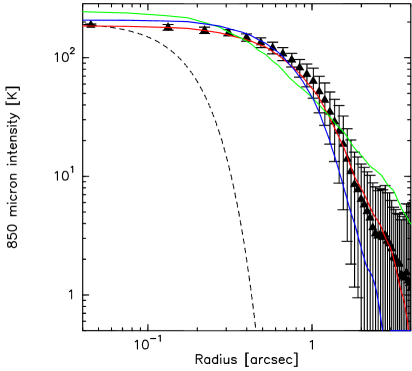
Figure 2: Radial profile of the Sgr B2(N)-SMA1 component, with errorbars denoting the rms in circular annuli. Overlaid are three models with different density distributions (red: Plummer; blue: Gaussian; green: power-law). The beam is depicted as a dashed Gaussian.

It remains unclear whether the Plummer profile, which is also used to describe density profiles of star clusters, has any relevance to an evolving star cluster, or whether the cluster loses its memory of the gas density profile in the subsequent dynamical evolution. The model has a mass of around 3000 M_⊙ inside a radius of 11500 AU (0.056 pc), which represents an average density of $4\times 10^{6}$ M_⊙ pc^-3. This is only the mass contained in the gas, and does not include the mass of the already formed compact objects providing the luminosity. Sgr B2(N) might represent a very young, embedded stage in the formation of a massive star cluster.

5 Discussion

Our SMA observations resolve the Sgr B2(M) and (N) cores into fourteen compact submillimeter continuum components. The two cores display very different morphologies. The source Sgr B2(N)-SMA1 is located north-east of the centimeter source K2, with an offset of $\sim$0.2^′′. The continuum observations at 1.3 cm having a resolution of 0.25^′′ (Gaume et al. 1995) and at 7 mm a resolution of 0.1^′′ (Rolffs et al. 2011) also detected a compact component centered on K2. We failed to detect any submillimeter continuum emission associated with sources K1, K3, and K4. Sgr B2(N)-SMA2 is a high-mass dust core.

In contrast to Sgr B2(N), a very fragmented cluster of high mass submillimeter sources is detected in Sgr B2(M). In addition to the two brightest and most massive components, Sgr B2(M)-SMA1 and Sgr B2(M)-SMA2, situated in the central region of Sgr B2(M), ten additional sources are detected, which indicates that there has been a high degree of fragmentation. The sensitivity of 0.021 Jy beam^-1 in our observations corresponds to a detectable gas mass of 1.2 M_⊙, but the observations are likely to be dynamic-range-limited, so it is difficult to determine the clump mass function in Sgr B2(M) down to smaller masses.

The estimated column densities ($10^{25}$cm^-2=33.4 g cm^-2) in both the homogeneous starforming region Sgr B2(N) and the clustered Sgr B2(M) region are well in excess of the threshold of 1 g cm^-2 for preventing cloud fragmentation and formation of massive stars (Krumholz & McKee 2008). The source sizes and masses derived from Gaussian fitting, assuming a spherical source, lead to volume densities in excess of $10^{7}$cm^-3 for all submillimeter sources detected in the SMA images. Assuming a gas temperature of 150 K, the thermal Jeans masses are less than 10 M_⊙, but the turbulent support is considerable. The large column densities, the gas masses, and the velocity field (Rolffs et al. 2010) suggest that the submillimeter components in the two regions are gravitationally unstable and in the process of forming massive stars. This process seems more advanced in Sgr B2(M), which is also reflected in the large number of embedded UC Hii regions found there. However, star formation in Sgr B2(N) does not appears to have progressed very far, a conclusion also supported by the presence of only one UC Hii region embedded in one of the two clumps studied here. The observations also showed that massive star formation taking place in the two clumps with outflow ages of $\sim 10^{3}$ and $\sim 10^{4}$ years for Sgr B2(N) and Sgr B2(M) clumps, respectively (Lis et al. 1993). If one can generalize these two examples, and if they provide snapshots in time of the evolution of basically equal cores, it seems that a massive star forms first in a relatively homogeneous core, another example with Plummer density profile and without fragmentation being the high-mass core G10.47 (Rolffs et al., in prep.), followed by fragmentation or at least visible break-up of the core and subsequent star formation, perhaps aided by radiative or outflow feedback from the first star. This scenario may well apply to extremely high-mass cluster forming cores or to special environments only, since high-mass IRDCs have been shown to fragment early (Zhang et al. 2009).

References

- Belloche, (2008) Belloche, A., Menten, K. M., Comito, C., et al. 2008, A&A, 482, 179
- Carlstrom (89) Carlstrom, J. E., & Vogel, S. N. 1989, A&A, 377, 408
- (3) de Pree, C. G., Goss, W. M., & Gaume, R. A. 1998, ApJ, 500, 847
- Friedel, (2004) Friedel, D. N., Snyder, L. E., Turner, B. E., Remijan, A. 2004, ApJ, 600, 234
- (5) Gaume, R. A., Claussen, M. J., de Pree, C. G., Goss, W. M., Mehringer, D. M. 1995, ApJ, 438, 776
- Hildebrand, (1983) Hildebrand, R. H. 1983, QJRAS, 24, 267
- Hollis, (2003) Hollis, J. M., Pedelty J. A., Boboltz D. A. et al. 2003, ApJ, 596, L235
- Jones, (2008) Jones, P. A., Burton, M. G., Cunningham, M. R., et al. 2008, MNRAS, 386, 117
- Krumholz, (2008) Krumholz, M. R., & McKee, C. F. 2008, Nature, 451, 1082
- Lis et al., (1991) Lis, D. C., Carlstrom, J. E., & Keene, J. 1991, ApJ, 380, 429
- (11) Lis, D. C., Goldsmith, P. F., Carlstrom, J. E., Scoville, N. Z. 1993, ApJ, 402, 238
- (12) Liu, Sheng-Yuan, & Snyder, L.E. 1999, ApJ, 523, 683
- Mehringer et al., (1997) Mehringer, D. M., & Menten, K. M. 1997, ApJ, 474, 346
- Nummelin (1998) Nummelin, A., Bergman, P., Hjalmarson, A., et al. 1998, ApJS, 117, 427
- Ossenkopf & Henning (1994) Ossenkopf, V., & Henning, T. 1994, A&A, 291, 943
- Qin (2008) Qin, Sheng-Li, Zhao, Jun-Hui, Moran James M., et al. 2008, ApJ, 677, 353
- reid et al., (2009) Reid, M. J., Menten, K. M., Zheng, X. W., et al. 2009, ApJ, 705, 1548
- Rolffs (2010) Rolffs, R., Schilke, P., Comito, C., et al., 2010, A&A, 521, L46
- Rolffs et al. (2011) Rolffs, R., Schilke, P., Wyrowski, F., et al. 2011, A&A, 529, 76
- Sault et al. (1995) Sault, R. J., Teuben, P. J., & Wright, M. C. H. 1995, in ASP Conf. Ser. 77, Astronomical Data Analysis Software and Systems IV, ed. R. A. Shaw, H. E. Payne, & J. J. E. Hayes (San Francisco, CA: ASP), 433
- Schuller et al. (2009) Schuller, F., et al. 2009, A&A, 504, 415
- Snyder et al. (1994) Snyder, L. E., Kuan, Y.-J., & Miao, Y. 1994, in The Structure and Content of Molecular Clouds, ed. T. L. Wilson & K. J. Johnston (Berlin: Springer), 187
- Zhang et al. (1994) Zhang, Q., Wang, Y., Pillai, T., & Rathborne, J. 2009, ApJ, 696, 268